-28- Abstract — We introduce a hybrid system composed of a convolutional neural network and a discrete graphical model for image recognition. This system improves upon traditional sliding window techniques for analysis of an image larger than the training data by effectively processing the full input scene through the neural network in less time. The final result is then inferred from the neural network output through energy minimization to reach a more precize localization than what traditional maximum value class comparisons yield. These results are apt for applying this process in a mobile device for real time image recognition.
Keywords — Computer vision, Image recognition, Deep neural networks, Graphical models, Mobile device.
I. INTRODUCTION
YBRIFD intelligent systems have consistently shown benefits that outperform those of their individual components in many tasks, especially when used along neural computing [1]. In recent years, two main areas of computer vision have gained considerable strength and support: On one side, soft computing techniques based on non-exact but very accurate machine learning models like neural networks, which have been successful for high level image classification [7]. Contrasting these systems, computer vision techniques modeled by graphical models have enjoyed great reception when performing low level image processing tasks such as image completion [6]. In this paper, we combine both of these techniques to successfully classify and localize a region of interest within an input image.
We use Convolutional Neural Networks (CNN) [3] for the classification of image content. CNNs have become a general solution for image recognition with variable input data, as their results have outclassed other machine learning approaches in large scale image recognition tasks [4]. Paired to this CNN classifier, we use energy minimization of a Markov Random Field (MRF) [8] for inference and localization of the target within the image space. Graphical models such as this have been implemented in areas of computer vision where the relationship between neighboring regions plays a crucial role [2].
We review the implementation of this system specifically within a mobile device. With the increasing use of mobile
hardware, it has become a priority to provide these devices with computer vision capabilities. Due to the high computational requirements, this need has mostly been met by outsourcing the analysis to a remote server over the Internet. This approach introduces large delays and is hardly appropriate when interactivity and responsiveness are paramount. Embedded environments have intrinsic architecture constraints which require algorithms to make the best use of the available computing capacity. The proposed system exploits this specific platform by reducing the overall required memory throughput via a parallel execution approach. This is achieved by applying layer computations over the entire image space, as opposed to running smaller patches individually, as is common with the sliding window approach normally used in this type of image classification.
The structure of this work is as follows: In Section 2, some background knowledge is reviewed detailing the functionality of CNNs and window analysis in general. We then introduce in Section 3 an optimized approach for the techniques previously discussed, including the architecture constraints that must be made to implement the proposed system. Section 4 goes over the discretization of the system and the inference process for obtaining the final output result. Section 5 continues with the results obtained from the proposed method and a brief comparison with other alternative approaches. Finally, Section 6 concludes by discussing the observations made and some additional applications where this system can be used in.
II. BACKGROUND
In this section, a brief description of CNNs and their layer types is given, as well as an overview of the traditional sliding window approach.
A.Convolutional Neural Networks
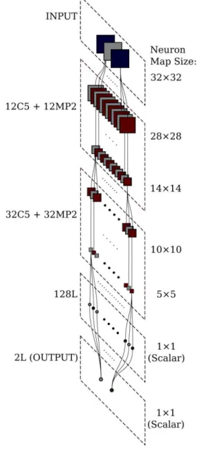
The network on which our system is based upon is a standard CNN. Figure 1 depicts the layer structure of such a network, and it is the reference architecture used throughout this paper to describe the concepts of the framework presented.
In the initial stages of the CNN, a neuron consists of a two-dimensional grid of independent computing units, each producing an output value. As a result, every neuron will itself output a grid of numerical values, a data structure in referred to as a map. When applying CNNs to image analysis, these
Neural Networks through Shared Maps in
Mobile Devices
William Raveane, María Angélica González Arrieta,
Universidad de Salmanca, Spain
H
-29- maps represent an internal state of the imageafter being processed through a connective path leading to that particular neuron. Consequently, maps will usually bear a direct positional and feature-wise relationship to the input image space. As data progresses through the network,
Fig. 1. A typical convolutional neural network architecture, with three input neurons for each color channel of an analyzed image patch, two feature extraction stages of convolutional and max-pooling layers, and two linear layers to produce a final one-vs-all classification output.
however, this representation turns more abstract as the dimensionality is reduced. Eventually, these maps are passed through one or more linear classifiers, layers consisting of traditional single unit neurons which output a single value each. For consistency, the outputs of these neurons are treated as single pixel image maps, although they are nothing more than scalar values in .
B.CNN Layer Types
The first layer in the network consists of the image data to be
analyzed, usually composed as the three color channels. The notation is used to describe all subsequent layers,
where is the neuron map count of layer ,
denotes the layer type group (Convolutional, Max-Pooling, and Linear), and is the parameter value for that layer.
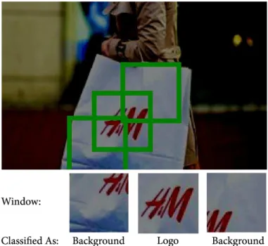
Fig. 2. Visualization of the first three neuron maps at each stage of the CNN. Note the data size reduction induced at each stage. The output of this execution consists of two scalar values, each one representing the likelihood that the analyzed input image belongs to that neuron’s corresponding class. In this case the logo has been successfully recognized by the higher valued output neuron for class “Logo”.
The first part of every feature extraction stage is a convolutional layer. Here, each neuron linearly combines the convolution of one or more preceding maps. The result is a map slightly smaller than the input size by an amount known as the kernel padding, which arises from the boundary conditions of the valid convolution algorithm. It is defined as , where is the convolutional kernel size of layer . Therefore, the layer's map size will be given
by , where is the the preceding
layer's map size.
-30- inversely proportional to said parameter by . The data may then be passed to one or more additional feature extractors.
Linear layers classify feature maps extracted on preceding layers through a linear combination as in a perceptron -- always working with scalar values -- such that at every layer of this type.
Finally, the output of the final classification layer decides the best matching label describing the input image. Fig. 2 shows the information flow leading to this classification for a given image patch, where the CNN has been trained to identify a particular company logo.
C.The Sliding Window Method
Recognition of images larger than the CNN input size is achieved by the sliding window approach. This algorithm is defined by two quantities, the window size , usually fixed to match the CNN's designed input size; and the window stride , which specifies the distance at which consecutive windows are spaced apart. This stride distance establishes the total number of windows analyzed for a given input image. For an image of size , the window count is given by:
Figure 3 shows this method applied on an input image
downsampled to , extracting windows of for
the simple case where . A network analyzing this image would require 40 executions to fully analyze all extracted windows. The computational requirement is further compounded when a smaller stride is selected -- an action necessary to improve the resolving power of the classifier: at , 464 separate CNN executions would be required.
Fig. 3. An overview of the sliding window method, where an input image is subdivided into smaller overlapping image patches, each being individually analyzed by a CNN. A classification result is then obtained for each
individual window.
III. OPTIMIZED NETWORK EXECUTION
The method proposed introduces a framework where the stride has no significant impact on the execution time of the stages, as long as the selected stride is among a constrained set of possible values. This is achieved by allowing layers to process the full image as a single shared map instead of individual windows. Constraints in the possible stride values will result in pixel calculations to be correctly aligned throughout the layers.
A.Shared Window Maps
CNNs have a built-in positional tolerance due to the reuse of the same convolutional kernels over the entire neuron map. As a result of this behavior, their output is independent of any pixel offset within the map, such that overlapping windows will share convolved values. This is demonstrated in Fig. 4.
Fig. 4. Two adjacent windows extracted from an input image, passed through the 12C5 + 12MP5 feature extractor. A detailed view of the convolved maps in the overlapping top-right and bottom-left quarters of each window shows that these areas fully match.
This leads to the possibility of streamlining the feature extractors by running their algorithms over the full input image at once. Hence, each neuron will output a single map shared among all windows, where subdivisions of this map would normally match the outputs of the corresponding windows, had they been executed separately as in the traditional method. This greatly reduces the expense of calculating again convolutions on overlapping regions of each window. Figure 5 shows an overview of the shared map process, which passes the input image in its entirety through each stage of the network.
-31- consists of image maps where each pixel yields the relative position of all simultaneously classified windows.
Similar to the per-window execution method, the intensity value of a pixel in the output map represents the classification likelihood of the corresponding window. Note how the relative position of the logo in the input image has been discovered after only one shared map execution of the network. An account of the window size and stride is also on
Fig. 5. The shared map execution method for a convolutional neural network, where each layer processes an entire image in a single pass, and each neuron is now able to process maps with dimensions that far exceed the layer’s designed input size.
display, illustrating how it evolves after each layer, while the total window count remains the same. Here, the correspondence of each window in the input image can be traced to each one of the pixels in the output maps.
B.Window Configuration
The operation of the shared map process relies greatly on the details of the dimensionality reduction occurring at each layer within the network. For this reason, it is necessary to lay certain constraints that must be enforced when choosing the optimum sliding window stride.
At each layer, the window size and stride are reduced until
Fig. 6. The CNN layers and their effect on the window pixel space, illustrated in
one dimension for simplicity. Two successive 32×32 windows W1 and W2 are shown. Overlapping pixels at each layer are shaded. Starting with an input layer window stride T0 = 4, the final output layer results in a packed T6 = 1 window stride, so that each output map pixel corresponds to a positional shift of 4 pixels in the input windows, a relationship depicted by the column paths traversing all layers.
-32- Where the window size and its stride at layer depends on the various parameters of the layer and the window size and stride values at the preceding layer. This equation set can be applied over the total number of layers of the network, while keeping as the target constraint that the final size and stride must remain whole integer values. By regressing these calculations back to the input layer , one can find that the single remaining constraint at that layer is given by:
In other words, the input window stride must be perfectly divisible by the product of the pooling size of all max-pooling layers in the network. Choosing the initial window stride in this manner, will ensure that every pixel in the final output map is correctly aligned throughout all shared maps and corresponds to exactly one input window. Fig. 6 follows the evolution of the window image data along the various layers of the sample network architecture, showing this pixel alignment throughout the CNN.
IV. DISCRETE INFERENCE OF CNNOUTPUT
The output from the convolutional neural network as seen in Fig. 5 consists of multiple individual maps, where each one embodies a visual depiction of the relative confidence, per-class, that the system has for every window sampled.
The common practice to obtain a final classification from an output value set as seen in Fig. 5 is to identify which class has a higher output value from the CNN at each each window (here, each pixel in the output map). While efficient, results from this procedure are not always ideal because they only take into account each window separately.
Furthermore, maximum value inference is prone to false positives over the full image area. Due to their non-exact nature, neural network accuracy can decrease by finding patterns in random stimuli which eventually trigger neurons in the final classification layer. However, such occurrences tend to appear in isolation around other successfully classified image regions. It is therefore possible to improve the performance of the classifier by taking into account nearby windows.
There exist many statistical approaches in which this can be implemented, such as (i) influencing the value of each window by a weighted average of neighboring windows, or (ii) boosting output values by the presence of similarly classified windows in the surrounding area. However, we propose
discrete energy minimization through belief propagation as a more general method to determine the final classification within a set of CNN output maps. The main reason being that graphical models are more flexible in adapting to image conditions and can usually converge on a globally optimal solution.
A.Pairwise Markov Random Field Model
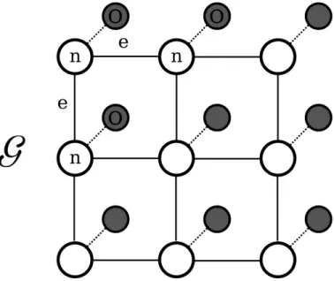
Images can be treated as an undirected cyclical
graph , where nodes represent an entity such
as a pixel in the image, and graph edges represent the relationship between these nodes. If, for simplicity, 4-connectivity is used to represent the relationship between successive nodes in a graph; then each node will be connected to four others corresponding to its neighbors above, below, and to each side of the current element.
The output space of the convolutional neural network can therefore be represented in this manner through a graph. However, instead of describing pixel intensity values, each node in the graph represents the classification state of the corresponding window. This state takes on a discrete value
among a set of class labels corresponding
to the classification targets of the CNN. Thus, each node in the graph can take on one of several discrete values, expressing the predicted class of the window that the node represents. Fig. 7 displays the structure of such a graph.
Fig. 7. A subset of the MRF graph G formed by the CNN output space, where each node ni represents the classification state of a corresponding window analyzed with the network, whose outputs are implemented into this system as the observed hidden variables O. Nodes have a 4-connectivity relationship with each other represented by the edges eij thus forming a grid-like cyclical graph.
-33- property in the graph nodes where there is a dependency between successive nodes. Therefore, this graph follows the same structure as an MRF, and any operations available to this kind of structure will be likewise applicable to the output map.
B.Energy Allocation
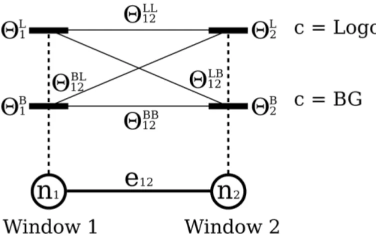
To implement energy minimization on an MRF, it is necessary to assign energy potentials to each node and edge. These energies are usually adapted from observed variables, and in this case, they correspond to the values of the output maps and combinations thereof. Therefore, MRF optimization over a graph can be carried out by minimizing its Markov random energy , given by:
Here, corresponds to the singleton energy potential of
node , and is a pairwise potential between
nodes and . Starting from the CNN output map observations, the singleton potentials can be assigned as:
Where is the total number of classes in set (2 in the sample CNN architecture), and is the observed CNN value
for window and class . In this manner,
each value is an MSE-like metric that measures how far off from ideal training target values did the CNN classify window as. Thus, a lower potential value will be assigned to the most likely class, while a higher potential value will be given to other possible classes at this node.
Pairwise potentials can be defined as:
Where each value is a straightforward distance metric that measures the jump in CNN output values when switching from class to class between windows and . Thus, these potentials will be small if the same class is assigned to both nodes, and large otherwise. Fig. 8 shows all energy assignments per node pair.
Fig. 8. A detail of the potential energies assigned to each of two nodes {n1 , n2} connected by edge e12 . The singleton potentials Θia correspond to the energy associated with node i if assigned to class a, and the pairwise potentials Θijab are the changes in energy that occur by assigning class a to node ni and class b to node nj .
It is worth noting that these pairwise potentials between neighboring windows (nodes) are the only feature that sets apart this process from the traditional winner-takes-all approach which would otherwise be implemented through the minimization of the energy in the singleton potentials by themselves.
C.Energy Minimization by Belief Propagation
Applying Belief Propagation [5] to find the lowest possible energy state of the graph will now yield an equilibrium of class assignments throughout the image output space.
Due to the cycles inherent of image-bound graphs, a special variation of the algorithm must be used, in this case Loopy Belief Propagation [5]. This variation requires the minimization to be run several times until the solution converges and an equilibrium is found. However, due to various existing optimizations for this algorithm, this process is very straightforward and can be solved in polynomial time.
V. RESULTS
The test application is developed for the Android mobile OS as an OpenGL ES shader which makes use of the available computing capabilities of the device GPU. The main logic of the system is placed within a fragment shader running the CNN per-pixel over a Surface Texture memory object. The test device is equipped with a quad core 1.3 GHz Cortex-A9 CPU with a 12-core 520 MHz Tegra 3 GPU. This SoC architecture embeds 1 Gb of DDR2 RAM shared by both the CPU and GPU.
6--34- connectivity between nodes such that each window is also aware of window classifications at the corresponding larger and smaller scale steps. Table 1 gives a summary of the results obtained from this setup.
Fig. 9. Comparison of the final “Logo” classification and localization, applying the classical maximum value per class extraction vs. our proposed energy minimization inference method on the two CNN output maps introduced in Figure 5
It is of great interest to note the final configuration. Regardless of the fact that there is no overlap at this stride, a 3.0 speedup is still observed over running the windows individually. This is due to the inherent reduction in memory bandwidth through the system's pipelined execution approach, where the entire image needs to be loaded only once per execution. This contrasts the traditional approach where loading separate windows into memory at different times requires each to be individually sliced from the original memory block -- a very expensive operation in the limited memory throughput of mobile devices.
Server platforms have a restriction in the PCIe bus speed between the CPU and GPU, but instead offer very fast local memory access within the GPU. As a result, these architectures would allow window extraction at lower relative latencies. The SoC architecture of mobile devices do not face similar CPU to GPU memory bottlenecks, as these chips are usually located within the same circuit. Their lower energy requirements, however, force local memory access to be radically slower. Therefore, this architecture favors the parallel usage of data blocks, a fact which the system we have presented exploits in full. As such, we consider it to be a mobile-first oriented algorithm, although it would offer likewise improvements in other platforms.
The results of the inference system are more of a qualitative nature, as it is difficult to objectively establish a ground truth
basis for such experiments. This system aims to localize classified windows, therefore it is subject to an interpretation of which windows cover enough of the recognition target to be counted as a true positive. Regardless, Table 2 gives an indicative comparison of the system against the competing techniques previousy described. Fig. 9 shows a visual comparison.
VI. CONCLUSIONS
A system for the optimization of convolutional neural networks has been presented for the particular application of mobile image recognition. The performance figures presented in Table 1 correspond to a device architecture which, at the time of this work, is a commonly available specification on end user devices. It must be noted that with the rapid growth that is being observed in mobile hardware capabilities, the effects of these optimizations are likely to grow in their significance. GPUs capable of new technology will extend the reach of the parallel-wise optimizations described. Relevant advancements in this area would include things such as heterogeneous parallel processing via OpenCL EP and zero-copy memory transfer between the camera and GPU through tighter SoC integration. General availability of such technologies will open an ever larger possibility of mobile computer vision opportunities.
Although a simple logo classification task was used here as a sample application, CNNs allow for many other image
TABLEI SPEEDUP RESULTS
T0 W (L) W (P) OC T (PW) T (SM) Speedup
4×4 464 3,712 98% 29,730 1,047 28.4x
8×8 112 896 94% 7,211 387 18.6x
12×12 60 480 86% 3,798 311 12.2x
16×16 32 256 75% 2,051 240 8.5x
20×20 24 192 61% 1,536 252 6.1x
24×24 15 120 44% 945 203 4.7x
28×28 15 120 23% 949 200 4.7x
32×32 8 64 0% 514 171 3.0x
Results of tests with several input layer stride T0 configurations, from the closest packed 4×4 to the non-overlapping 32×32 layouts. A total window count at each pyramid level W (L), and over the full 8 level pyramid W (P), as well as the window overlap coverage OC per input map is given for each of the stride selections. An average over 20 test runs for each of these configurations was taken as the execution time in milliseconds for each of the methods described herein – the traditional per-window execution method T (PW), and our shared map technique T (SM). A speedup factor is calculated showing the performance improvement of our method over the other.
TABLEII INFERENCE RESULTS
Algorithm Accuracy PPV F1
Maximum Value 0.942 0.341 0.498
Weighted Average 0.964 0.391 0.430
Neighbor Boosting 0.972 0.489 0.591
Energy Minimization 0.981 0.747 0.694
-35- recognition tasks to be carried out. Most of these processes would have great impact on end users if implemented as real time mobile applications. Some examples where CNNs have been successfully used and their possible mobile implementations would be (i) text recognition for visually interactive language translators, (ii) human action recognition for increased user interactivity in social applications, or even (iii) traffic sign recognition for embedded automotive applications. Any of these applications could be similarly optimized and discretized by the system presented here.
In addition to the CNN classifier, the MRF model is very flexible as well and its implementation can be adjusted to domain-specific requirements as needed by each application. For example, a visual text recognizer might implement pairwise energy potentials which are modeled with the probabilistic distribution of character bigrams or n-grams over a corpus of text, thereby increasing the overall text recognition accuracy.
Furthermore, although the analysis of a single image has been discussed, this system is similarly extensible to multiple images processed together. The most common example of this is the analysis of a multi-scale image pyramid, something vital within mobile applications as variable distances between the camera and its target will cause the object to be observed at different sizes within the analyzed image. In such a case, the MRF would be extended to a 6-connectivity 3D grid, where nodes would be equally aware of window classifications at the corresponding larger and smaller scale steps.
Therefore, we believe this to be a general purpose mobile computer vision framework which can be deployed for many different uses within the restrictions imposed by embedded hardware, but also encouraging the limitless possibilities of mobile applications.
REFERENCES
[1] Borrajo, M.L., Baruque, B., Corchado, E., Bajo, J., Corchado, J.M.: Hybrid neural intelligent system to predict business failure in small-to-medium-size enterprises. International Journal of Neural Systems 21(04), 277–296 (2011)
[2] Boykov, Y., Veksler, O.: Graph Cuts in Vision and Graphics: Theories and Applications. In: Paragios, N., Chen, Y., Faugeras, O. (eds.) Handbook of Mathematical Models in Computer Vision, pp. 79–96. Springer US (2006)
[3] Ciresan, D.C., Meier, U., Masci, J., Gambardella, L.M., Schmidhuber, J.: Flexible, High Performance Convolutional Neural Networks for Image Classication. In: Proceedings of the Twenty-Second International Joint Conference on Artificial Intelligence. pp. 1237–1242 (2011) [4] Ciresan, D.C., Meier, U., Gambardella, L.M., Schmidhuber, J.:
Convolutional Neural Network Committees For Handwritten Character Classification. In: 11th International Conference on Document Analysis and Recognition. ICDAR (2011)
[5] Felzenszwalb, P.F., Huttenlocher, D.P.: Efficient Belief Propagation for Early Vision. International Journal of Computer Vision 70(1), 41–54 (May 2006)
[6] Komodakis, N., Tziritas, G.: Image completion using efficient belief propagation via priority scheduling and dynamic pruning. Image Processing, IEEE Transactions on 16(11), 2649–2661 (Nov 2007) [7] Krizhevsky, A., Sutskever, I., Hinton, G.E.: ImageNet Classification
with Deep Convolutional Neural Networks. pp. 1106–1114. No. 25 (2012)
[8] Wang, C., Paragios, N.: Markov Random Fields in Vision Perception: A Survey. Rapport de recherche RR-7945, INRIA (September 2012)
William Raveane is a Ph.D. candidate in Computer Engineering at the University of Salamanca, Spain, currently researching mobile image recognition through deep neural networks. He has also worked for several years in private companies in various topics ranging from computer vision to visual effects.