CONTROL OF NONLINEAR PROCESS
USING NEURAL NETWORK BASED
MODEL PREDICTIVE CONTROL
PIYUSH SHRIVASTAVA
PG Scholar, Control Systems, Department. Of Electrical Engineering, Jabalpur Engineering College, Jabalpur, Madhya Pradesh 482001, India
Dr.A.TRIVEDI
Reader, Department of electrical Engineering, Jabalpur Engineering College, Jabalpur, Madhya Pradesh 482001, India
Abstract:
This paper presents a Neural Network based Model Predictive Control (NNMPC) strategy to control nonlinear process. Multilayer Perceptron Neural Network (MLP) is chosen to represent a Nonlinear Auto Regressive with eXogenous signal (NARX) model of a nonlinear system. NARX dynamic model is based on feed-forward architecture and offers good approximation capabilities along with robustness and accuracy. Based on the identified neural model, a generalized predictive control (GPC) algorithm is implemented to control the composition in a continuous stirred tank reactor (CSTR), whose parameters are optimally determined by solving quadratic performance index using well known Levenberg-Marquardt and Quasi-Newton algorithm. NNMPC is tuned by selecting few horizon parameters and weighting factor. The tracking performance of the NNMPC is tested using different amplitude function as a reference signal on CSTR application. Also the robustness and performance is tested in the presence of disturbance on random reference signal.
Keywords: Continuous Stirred Tank Reactor; Neural Network based Predictive Control; Nonlinear Auto Regressive with eXogenous signal.
1. Introduction
Model predictive control (MPC) techniques have been recognized as efficient approaches to improve operating efficiency and profitability. It has become the accepted standard for complex control problems in the process industries. It can be used for the control of non-linear systems if they are working around an operating point. However, if the operating point is moved away from the nominal work point, the controller is less effective, or even detrimental to the system operation. One solution to this kind of control problem is to develop a non-linear model predictive control strategy. NN have been shown to have good approximation capability for non-linear systems [1]. A large number of predictive control schemes have been developed based on Multi Layer Perceptron (MLP) neural network models since 1990.The key to the successful application of non-linear MPC based on a neural network model is an accurate nonlinear model and an efficient optimization algorithm. The back propagation learning algorithm, commonly used in MLP, is essentially a non-linear steepest descent algorithm [2].
The aim of controller design is to construct a controller that generates control signals that in turn generate the desired plant output subject to given constraints. Predictive control tries to predict, what would happen to the plant output for a given control signal. In this way, we know in advance, what effect the control will have, and by this knowledge the best possible control signal is chosen. Whats the best possible outcome depends on the given plant and situation, but the general idea is the same.
An algorithm called Generalized predictive control [3] was introduced in to implement predictive control, and is
with using a neural network model of the plant to do predictive control. Firstly the linear case of predictive control is discussed. Then aspects of modeling of the plant with a neural network are investigated. This is also referred to as System Identification.
2. Generalized Predictive Control
The generalized predictive control (GPC) is discussed in [3]. It is a receding horizon method. For a series of projected controls the plant output is predicted over a given number of samples, and the control strategy is based upon the projected control series and the predicted plant output. Some of the features of the GPC are summarized as follows and the detailed description is provided in [3]:
The objective is to find a control time series that minimizes the cost function:
2 2 2
N N2
i=1 i=1
(
) r (t+i)
(
1)
GPC
J
E
y t i
u t i
(1)
subject to the constraint that the projected controls are a function of available data. N2 is the costing horizon, ρ is the control weight. The expectation of (1) is conditioned on data up to time t. The plant output is denoted y, the reference r, and the control signal u. ∆ is the shifting operator 1 – q-1 such that,
( ) ( ) ( 1)
u t u t u t
(2)
The first summation in the cost function penalizes deviation of the plant output y(t) from the reference r(t) in the time interval t + 1 ≤ t ≤ t + N2. The second summation penalizes control signal change ∆u(t) of the projected control series.
Furthermore, so called control horizon, Nu ≤ N2 is introduced. Beyond this horizon the projected control increments ∆u are fixed at zero:
( 1) 0
u t i
i
N
u (3)The projected control signal will remain constant after this time. This is equivalent to placing an effectively infinite weight on control changes for t > Nu. Small values of Nu generally result in smooth and sluggish actuations, while larger values provide more active controls. The use of a control horizon Nu < N2 reduces the computation burden [3].
2.1 The Control Law for Linear Systems
Let first derive the control law for a linear system that can be modeled by the Controlled Auto-Regressive and Moving Average Model (CARIMA) model:
1 1 1 1
(
) ( )
(
) ( )
(
) ( ) /
A q
y t
q B q u t
C q
t
(4)Where,
( )t is an uncorrelated random sequence. Let’s introduce,2
[ (
1), (
2),..., (
)]
TN
y
y t
y t
y t
N
(5)2
[ (
1), (
2),..., (
)]
Tw
r t
r t
r t
N
(6)2
[
( ),
(
2),...,
(
1)]
Tu
u t
u t
u t
N
(7)and let yt represent data up to time t, now note that
2 2
||
N||
||
|| |
tJ
E
y
w
u
y
2 2
||
y
Nw
||
||
u
||
(8) where in turn,In linear case σ is independent of
u
and yN, and when minimizing the cost function, σ constitutes a constant value that can be ignored [4].y
ˆ
N can be separated in two terms:
y
ˆ
N
Gu
f
(10) where fis the free response, andGu
is the forced response.The free response is the response of the plant output as a result of the current state of the plant with no change in input. The forced response is the plant output due to the control sequence,
u
. The linearity allows for this separation of the two responses. The important fact is that fdepends on the plant parameters and yt (i.e. past values of u and y) while the matrix G only depends on the plant parameters. G does not change over time, and fcan be computed very efficiently. Using (8) and (10) we now have:2 2
||
N||
|| ||
J
y
w
u
||
Gu
f
w
||
2
|| ||
u
2
(
) (
)
T T
Gu
f
w
Gu
f
w
u u
(11)The minimization of the cost function on future controls results in the following control increment vector:
* 1
min
(
T)
T(
)
u
J
u
G G
I
G
wf
(12)and in the following current control signal:
( )
(
1)
T(
)
u t
u t
g
w
f
(13)where
g
Tis the first row of(
G G
T
I
)
1G
T.2.2 Non-linear Case
If the plant is nonlinear, the cost function (1) / (8) remains the same, but implementation of the algorithm is done in a different way [4]. The σ in equation (8) is not independent of
u
nory
ˆ
N for a nonlinear plant. It is however assumed that the effects of σ are small and can be ignored. Especially the prediction of the plant outputsy
ˆ
N based on the projected control seriesu
cannot be done in the same way.For a nonlinear plant the prediction of future output signals cannot be found in a way similar to (10). The relation of the control signal series to the plant output series is nonlinear, i.e. the multivariable function f that fulfils:
y
ˆ
N
f y u
( , )
t
(14)is nonlinear. Therefore free response from the forced response cannot be separated. To solve this problem
y
ˆ
N i.e. f in (14) is to be implemented in a different way. A nonlinear predictory
ˆ
N for future plant outputs in needed. This is where the neural network comes into play: The neural network is now facilitated to the workings of the function f in (14) to obtain the predictionsy
ˆ
N.Now neural network is trained to do a time series prediction of plant outputsy
ˆ
N for a given control signal time seriesu
. This will let us evaluate the GPC cost function (1) for a nonlinear plant. Using a suitable optimization algorithm on the projected control signal series with respect to the cost function, a control series that minimizes the cost function is obtained:
*
min
u
J
u
(15) The complete control algorithm iterates through these three steps: predict plant output times series yˆ
calculate cost function J
That is, first a control time series
u
is chosen. Using a model we look at what would happen if this series of control signals is used: the plant output yˆ can be predicted, then next a cost function (1) is used which shows how good or bad the outcome is. Then let the optimization algorithm choose a new control time seriesu
that is better by means of the cost function (1). Then number of iterations of these steps is done in order to find a series of control signals that is optimal with respect to the cost function (1).There are 3 distinctive components in this controller:
time series predictor of plant outputs
cost function
optimization algorithm
The cost function is given by (1). For the optimization algorithm the Levenberg-Marquardt (LM) and Quasi Newton (QN) algorithm have been used. Also in section 3, the time series predictor using a neural network model of the plant is discussed.
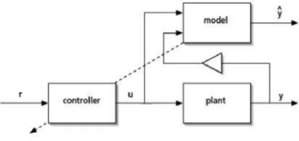
The complete system diagram is sketched in Figure1. The neural network model runs alongside the real plant and is used by the controller as discussed above to predict plant outputs to be used by the controller’s optimization algorithm.
Figure 1: Neural network based predictive controller
2.3 Control Horizon
As noted earlier in section 2, the control horizon Nu ≤ N2 limits the number of projected control signal changes such that
( 1) 0
u t j
,
j
N
uIf the control horizon is set to some value Nu < N2, the optimizer will only work on a series of Nu projected control signal changes, while evaluating a predicted plant output series that has N2 samples. Reducing Nu will reduce the computational burden, as it effectively reduces the dimension of the multidimensional variable that the optimizer works on.
3 Neural Network Predictive Control (NNMPC)
By the knowledge of the identified NARX model of the nonlinear plant which is capable of doing multi step ahead predictions, GPC algorithm is applied to control nonlinear process. The idea of GPC is to minimize cost function, J at each sampling point:
u
2
1
2 2 N
N
t=N i=1
ˆ
( , ( ))
(
) y (k+i)
(
1)
J t U k
r k i
u k i
(16)
With respect to the Nu future controls,
( )
[ ( )... (
u1)]
Tand subject to constraints:
2
(
)
u k
N
i
N
n
(18)Using the predictive control strategy with identified NARX model (NNMPC) it is possible to calculate the optimal control sequence for nonlinear plant. Here, term r(k+i) is the required reference plant output, ˆy (k+i)is predicted NN model output, u k( i 1) is the control increment, N1 and N2 are the minimum and maximum
prediction (or cost) horizons, Nu is the control horizon, and is the control penalty factor[4].
The predictive control approach is also termed as a receding horizon strategy, as it solves the above-defined optimization problem [5] for a finite future, at a current time and implements the first optimal control input as the current control input. The vector u = [u(k),u(k+1),…u(k + Nu-1)] is calculated by minimizing cost function, J at each sample k for selected values of the control parameters {N1, N2, Nu, }. These control parameters defines the predictive control performance. N1 is usually set to a value 1 that is equal to the time delay, and N2is set to define the
prediction horizon i.e. the number of time-steps in the future for which the plant response is recursively predicted.
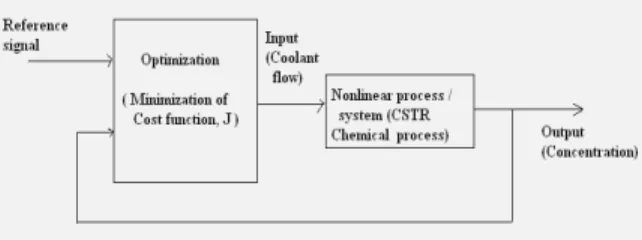
Figure 2: NNMPC principle applied to CSTR chemical process
The minimization of criterion, J in NNMPC is an optimization problem minimized iteratively. Similar to NN training strategies, iterative search methods are applied to determine the minimum.
(i+1) ( ) (i) (i)
=
i+
.d
(19) where,
( )i specifies the current iterate (number ‘i’), d(i)is the search direction and
(i)is the step size. Various types of algorithms exist, characterized by the way in which search direction and step size are selected. In the present work Newton based Levenberg–Marquardt (LM) and Quasi-Newton (QN) algorithms are implemented. The search direction applied in LM algorithm is:
i i i i
ˆ
(H[U (t)] + I)d = -G[U (t)]
(20)with Gradient vector and Hessian matrix as:
i ( ) ( ) i ( ) ( )
J(t,U(t))
G[U (t)] =
|
U(t)
U(t)
2
[U (t)]E(t)+2
( ) |
U(t)
i
i
U t U t
T
U t U t
U t
(21) 2 i2 ( ) ( )
T
( ) ( )
J(t,U(t)) H[U (t)] = |
U(t) ˆ
Y(t) U (t) ( ) = E(t) +2 |
U(t) U(t) U(t) ( )
i
i
U t U t
U t U t
while in case of QN algorithm it is as
d = -B G[U (t)]
(i) (i) i (22)where B(i) specifies the approximation of the inverse Hessian and G[U(i)(t)] is the gradient of the J with respect to the control inputs. In QN algorithm, the inverse Hessian is approximated directly from cost function, J and gradient contained in the past iterations. The most popular formula known as Broyden-Fletcher-Goldfarb-Shanno (BFGS) algorithm to approximate the inverse Hessian is used here[8]. QN is easier to implement as exact Hessian is not required and it further ensures fast convergence. The proposed scheme of implementing the NNMPC is shown in Figure 2.
Time Series Prediction with Neural Networks
The purpose of our neural network model is to do time series prediction of the plant output. Given a series of control signals
u
and past datay
t it is desired to predict the plant output series yN ((5) (7)).The network is trained to do one step ahead prediction[9], i.e. to predict the plant output yt+1 given the current control signal ut and plant outputy
t.The neural network will implement the function
y
ˆ
t1
f u y
( , )
t t (23)As it is discussed above, yt has to contain sufficient information for this prediction to be possible.It is assumed that yt is multivariable. One problem is that this method will cause a rapidly increasing divergence due to accumulation of errors. It therefore puts high demands on accuracy of the model. The better the model matches the actual plant the less significant the accumulated error. A sampling time as large as possible is an effective method to reduce the error accumulation as it effectively reduces the number of steps needed for a given time horizon. The neural network trained to do one step ahead prediction will model the plant. The acquisition of this model is also referred to as System Identification.
4 Simulation Results Discussion
Chemical Reactor
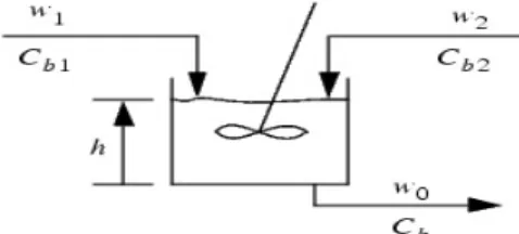
A continuous stirred tank reactor [10] shown in Figure 3 is used as the nonlinear plant on which the predictive algorithms are applied to control the nonlinear process.
Figure 3: Continuous Stirred Tank Reactor
The dynamic model of the system is
(24)
(25)
The objective of the controller is to maintain the product concentration by adjusting the flow w1 (t), w2 (t) =0.1.The level of the tank h is not controlled. The designed controller uses a neural network model to predict future CSTR responses to potential control signals. The training data were obtained from the nonlinear model of CSTR.
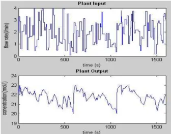
Figure 4: Input Output sequence for NNMPC
Figure 5: Prediction error using LM
Figure 6: NN output using LM
Figure 7: Plant output and Ref signal using LM
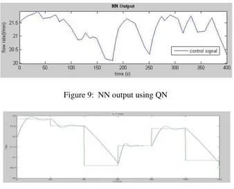
Figure 9: NN output using QN
Figure 10: Plant output and ref. signal using QN
Figure 4 show the plant input and output sequence of the plant, it is the regenerated training data by applying a series of random steps input to the simulated plant model.
In Figure (5, 8) prediction error is shown, it is the difference between the plant output and the output of the neural network plant model. This prediction error is used for the training of the neural network.
Neural Network plant model generates the control signal which actually is the one step ahead prediction of the controller and is shown in Figure (6, 9). Response graph showing the reference signal and tracking plant output using the iterative algorithms namely LM and QN are shown in Figure (7, 10).On analysis of these response graphs it is seen that the NNMPC strategy successfully tracks the random signal showing the robustness and successful set point tracking point tracking ability of the controller employed to CSTR.
5 Conclusion
In this paper the inclusion of dynamic neural models in predictive control for a benchmark nonlinear process, CSTR is presented. A NARX model was identified using MLP, and validated on the data generated from simulation of CSTR dynamic equations. This model represents the dynamics of the nonlinear CSTR and is used as nonlinear predictor in the discussed predictive control technique, NNMPC.
The control technique is tested on reference signals which exhibits, the possible nonlinear process dynamics occurring inside a real CSTR reactor. On analysis of the response graphs it can be seen that the NNMPC strategy successfully tracks the random reference signal.
The result obtained for the random reference signal illustrates and proves the tracking ability of controller. Also almost offset free and very close set point tracking is obtained using NNMPC strategy.
The NNMPC technique involves two algorithms namely LM and QN. On comparing the results obtained by both the algorithm it is seen that LM and QN algorithms behaves somewhat different from each other. In case of NNMPC employing LM algorithm, the control effort seems to be smoother than the NNMPC employing QN algorithm. But on the other hand tracking error in case of QN is little less than the prediction error obtained by using LM based NNMPC.
References
[1] Morari, M. and Lee, J. H. 1999. Model predictive control: past, present and future, Computers and Chemical Engineering, 23, 667-682. [2] L.G. Lightbody and G. W. Irwin, “Neural networks for nonlinear adaptive control, “in Proc. IFAC Symp. Algorithms Architectures
Real-Time Control, Bangor, U.K. pp. 1–13, 1992.
[3] D. W. Clarke, C. Mohtadi and P. S. Tuffs, “Generalized Predictive Control Basic Algorithm”, Automatica, Vol.23, no.2, pp: 137- 148, 1987.
[4] Garcia C. E. and Morari, M. 1982. Internal model control-I. “A unifying review and some new results,Industrial Engineering Chemical Process ”. Dev. 21, 308--323.
[5] X. Zhu, D.E. Seborg, “Nonlinear model predictive control based on Hammerstein models”, in. Proc. International Symposium on Process System Engineering, Seoul, Korea, pp. 995–1000, 1994.
[6] Vasičkaninova and M. Bakošova, “Neural network predictive control of a chemical reactor” Proceedings 23rd European Conference on Modelling and Simulation ©ECMS Javier Otamendi, Andrzej Bargiela, 2006.
[8] N. Kishor, “Nonlinear predictive control to track deviated power of an identified NNARX model of a hydro plant”. Expert Systems with Applications 35, 1741–1751, 2008.
[9] Tan, Y. and Cauwenberghe, A. “Non-linear one step ahead control using neural networks: control strategy and stability design”, Automatica, vol 32, no. 12, 1701-1706, 1996.
[10] J.J. Espionsa J. Vanderwalle, “Predictive Control using Fuzzy models”, Advances in soft Computing-engineering design and manufacturing, March. 1998. pp: 437-443.