ISSN 0104-6632 Printed in Brazil www.abeq.org.br/bjche
Vol. 30, No. 01, pp. 105 - 116, January - March, 2013
Brazilian Journal
of Chemical
Engineering
MODELING OF AN INDUSTRIAL PROCESS OF
PLEUROMUTILIN FERMENTATION USING
FEED-FORWARD NEURAL NETWORKS
L. Khaouane
*, O. Benkortbi, S. Hanini and C. Si-Moussa
LBMPT, Université de Médéa, Phone: +213 07 94 68 73 84, Quartier Ain D’Heb, 26000, Médéa, Algeria.
E-mail: [email protected]
(Submitted: December 4, 2011 ; Revised: March 24, 2012 ; Accepted: May 8, 2012)
Abstract - This work investigates the use of artificial neural networks in modeling an industrial fermentation process of Pleuromutilin produced by Pleurotus mutilus in a fed-batch mode. Three feed-forward neural network models characterized by a similar structure (five neurons in the input layer, one hidden layer and one neuron in the output layer) are constructed and optimized with the aim to predict the evolution of three main bioprocess variables: biomass, substrate and product. Results show a good fit between the predicted and experimental values for each model (the root mean squared errors were 0.4624% - 0.1234 g/L and 0.0016 mg/g respectively). Furthermore, the comparison between the optimized models and the unstructured kinetic models in terms of simulation results shows that neural network models gave more significant results. These results encourage further studies to integrate the mathematical formulae extracted from these models into an industrial control loop of the process.
Keywords: Modeling; Pleuromutilin; Fermentation; Feed-forward neural networks.
INTRODUCTION
In an increasingly competitive worldwide antibiotic market faced with economic, environ-mental and safety constraints, the industrialists have to increase their antibiotic production quantitatively and qualitatively, and reduce their costs and their energy consumption. Moreover, due to the complexity and non-linearity of the phenomena (Potocnik and Grabec, 1999), a modeling of antibiotic production, which remains a challenging problem, is required.
Kinetic models, known as a white box strategy, provide an analytical expression relating the key characteristics of the physical system to its dynamic behavior. These models have been and are still extensively applied in fermentation processes (Benkortbi et al., 2007; Cruz et al., 1999; Paul and Thomas, 1996; Zangirolami et al., 1997). However,
in some cases, those models do not apply, due to the inherent non-linearity of the system, lack of experimental information, experimental inaccuracy, or deviations from ideal conditions (Feyo de Azevedo et al., 1997; Silva et al., 2008; Saraceno et al., 2009).
Artificial neural networks (ANN) have gained a great popularity in the last decade as an attractive alternative to the previous approach due to their high parallelism, robustness (Basheer and Hajmeer, 2000) and, more interestingly, their inherent ability to extract from experimental data the highly non-linear and complex relationships between the variables of the problem (Si-Moussa et al., 2008) without any detailed knowledge of the system (Bryjak et al., 2004).
penicillin fermentation. In the work of Shene et al. (1999), two different neural networks (a feed-forward black box neural network and a hybrid gray box neural network) were designed to predict the state variables in ethanol batch fermentation taking into account the effect of medium composition and temperature. Kovarova-Kovar et al. (2000) presented the use of a combination of predictive control and an ANN-model to optimize the industrial fed-batch process for commercial production of riboflavin (vitamin B2). However, in the paper of Huang et al. (2002), an auto-associative neural network model was presented for on-line fault detection in Virginiamycin production. Saraceno et al. (2009) simulated the fermentation of ricotta cheese whey for the production of ethanol by means of a multiple hybrid neural model (HNM), obtained by coupling a multilayer perceptron neural network to mass balance equations for lactose, ethanol and biomass.
This work is a part of research on modeling the diterpene antibiotic Pleuromutilin, which is a natural
product, obtained by fermentation of Pleurotus
mutilus, an edible mushroom. This compound is active against a variety of gram-positive bacteria and mycoplasmas and is an inhibitor of bacterial protein synthesis (Kavanagh et al., 1951; Egger and Reinshagen, 1976).
On the other hand, Pleuromutilin served as a lead structure in the development of several commercial antibiotics such as tiamulin and valnemulin used in
veterinary medicine (Hannan et al., 1997) and
retapamulin approved for the treatment of human skin infections (Hirokawa et al., 2008).
In this paper, we developed three feed-forward ANN models, in order to assess the difficult-to-measure quantities, such as concentrations of biomass, substrate and product, from easily measurable variables in a fed-batch mode. This would be very interesting for further applications to digital control of the process, or measurement devices, and thus improve the reproducibility of the process and increase the Pleuromutilin productivity.
MATERIALS AND METHODS
Data Collection, Pretreatment and Analysis
Nineteen complete sets of data were provided by Antibiotical, a subsidiary of the Algerian pharma-ceutical company Saidal, containing data on: biomass concentration (X), glucose consumption (S), Pleuromutilin concentration (P), pH evolution, and refractive index of the fermentation broth (RI).
The collected experimental data were interpolated using a cubic spline function when necessary and smoothed with a moving average digital filter. Without smoothing, the ANN tends to capture the noise in the system rather than the fundamental mechanisms of the underlying process (Laursen et al., 2007) which results in a lower efficiency and a longer time to train the ANN.
ANN Development Procedure
Models Description
A neural network (NN) is a computational framework that is inspired by biological neural systems. It consists of a number of interconnected simple processing units called artificial neurons. One
of the most popular neural network paradigms
applied to the modeling of a wide range of nonlinear systems, especially chemical and biological engi-neering processes, is the feed-forward back propagation neural network (FFNN) (Lee and Park, 1999; Silva et al., 2000), which has been used throughout this paper with forecasting horizon and supervised learning.
The proposed FFNN consists of three models that are characterized by the same general structure including an input layer, one or two hidden layers and an output layer for the prediction of biomass, glucose and Pleuromutilin concentration profiles during fermentation.
A set of input variables was identified for each model: pH, refractive index (RI), initial glucose concentration (S0), initial inoculum concentration (X0) and fermentation time (t). A preliminary analysis based on the improved stepwise methods used for testing the contributions of NN inputs revealed that these variables exhibited the highest influence on process performance; more details on this technique can be found in Gevrey et al. (2003).
The statistical analysis of input and output data is shown in Table 1.
Table 1: Statistical analysis of input and output data.
STD Mean
t (h) pH RI X0 (%)
S0 (g/l)
X (%) S (g/l)
P (mg of product/g of biomass)
Models Development
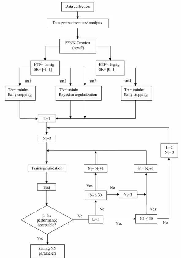
In this study, a procedure based on the development and optimization of the architecture of a feed-forward
network is advanced. It is based, as described in Figure 1, on the design of four FFNN sub-models which differ by the type of transfer function and the type of learning algorithm commonly used in biotechnology.
In order to make the training of the four sub-models more efficient by preventing the transfer function from becoming saturated and making the training of the networks very fast, all inputs and outputs were scaled in the range (SR) 0 to 1 and -1 to 1 depending on the hidden transfer function (HTF) used (log-sigmoid or hyperbolic tangent sigmoid, respectively), using the following scaling equation:
min
N max min min
max min
x x
x (y y ) * y
x x
⎛ − ⎞
= − ⎜ ⎟+
−
⎝ ⎠ (1)
where x is the normalized value of the parameter x N (t, pH, RI,X ,0 S , X, S or P); 0 xmax and xmin are the maximum and minimum values of x, respectively;
max
y and ymincan take the values 0 and 1 or -1 and 1. For all sub-models, the linear transfer function was attributed to the output layer.
Depending on the most successful and commonly used back propagation training algorithm, two enhancement generalization techniques were used. Over-fitting or poor generalization capability occurs when a neural network over learns during the training period. As a result, such a too well-trained model may not perform well on an unseen data set due to its lack of generalization capability. To overcome this problem, early stopping and Bayesian regularization methods were applied with the most successful Levenberg-Marquardt (MATLAB code trainlm) and Bayesian regulation (MATLAB code trainbr) back propagation training algorithms, respectively (The Mathworks Inc., 2010).
The early stopping technique is a very common practice in neural network training and often
produces networks that generalize well. This
technique is based on the division of data sets into three parts: training, validation, and test sets. The network is trained using the training set to minimize the error and checked with the validation set after each iteration to prevent over learning for the training set and loss of ability to generalize (Bishop, 1995; Pigram and MacDonald, 2000). As a final check, the test set is used on the network to make sure that the network performs and generalizes well (Hirschen and Schafer, 2006; Hagan et al., 1996; Asensio-Cuesta et al., 2010).
The Bayesian regularization is a more sophisticated approach to improve generalization. It was first used by MacKay (1991). This method not only minimizes a linear combination of squared errors and weights, rather than simply the squared errors, but also
modifies the linear combination so that, at the end of the training, the resulting network has good generalization qualities (MacKay, 1991; Danaher et al., 2004; Hagan et al., 1996; The Mathworks Inc., 2010).
In our work, the available data (551 samples) were randomly split into three distinct subsets, reserving 60% of the data (385 samples) for the training phase, 20% (83 samples) for the validation phase and the remaining 20% (83 samples) for the test phase.When early stopping was applied, the training and validation sets were used for the purposes described previously, whereas with Bayesian regularization the validation set was added to the training set to train the models. The test set for both techniques was used to test the generalization of the trained FFNN sub models.
In order to optimize the architecture for each sub-model, thus determining the number of hidden layers and the number of nodes in each layer, a trial-and-error procedure was implemented as described in Figure 1. The number of hidden layers (L) varied from 1 to 2 layers and the number of hidden neurons (N) in each layer varied from 3 to 30 neurons according to the forward method (Heaton, 2005).
The performances of various sub-models were evaluated in terms of the root mean squared error (RMSE) criterion. The RMSE was calculated using the following equation:
(
)
2cal exp
1
RMSE y y
N
= − (2)
where N is the total number of data; ycal represents the predicted output from the neural network model for a given input, while yexp is the experimental value.
The development procedure of the FFNN described above was carried out by elaborating a MATLAB program under MATLAB Neural Network Toolbox ver.7.10 (The Mathworks Inc., 2010). It was used to optimize the architecture of the three models utilized to predict the concentration profiles of biomass, glucose and product, respectively.
Comparison with Unstructured Kinetic Models
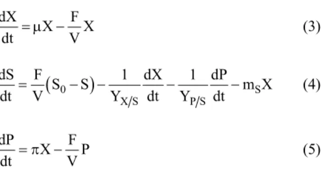
culture can be described by the following mass balance equations:
dX F
X X
dt = μ −V (3)
(
0)
SX S P S
dS F 1 dX 1 dP
S S m X
dt =V − −Y dt −Y dt − (4)
dP F
X P
dt = π −V (5)
where X, S and P are the concentrations of biomass, substrate and Pleuromutilin respectively; t is the current fermentation time; μ is the specific growth rate of biomass; π is the specific rate of product formation; V is the industrial bioreactor (culture) volume; S0 and F are the substrate concentration and feed rate of the medium added to the bioreactor, respectively; mS is the maintenance coefficient; YX/S is the yield of biomass per unit mass of substrate, and YP/S is the yield of product per unit mass of substrate.
As the volume V of the bioreactor used in the industrial production of Pleuromutilin is very large compared to the feed F, the term F/V is neglected and therefore the equations become (Pirt, 1979; Stanbury et al., 1999):
dX X
dt = μ (6)
S
X S P S
dS 1 dX 1 dP
m X
dt = −Y dt −Y dt − (7)
dP X
dt = π (8)
The specific rates of growth and Pleuromutilin formation were modeled by the following equations (Patnaik, 2001):
max S
S k X S
μ
μ = + (9)
max 2
S i
S
k S S k
π π =
+ + (10)
where kS is the Monod constant; ki is the inhibition constant, and μmax and πmax are the maximum values
of μ and π respectively.
Kinetic simulations were carried out by developing a MATLAB program based on four stages (Cutlip and Shacham, 2008; The Mathworks Inc., 2010): (a) give initial fixed values to the kinetic parameters and then integrate the differential equations using the ode45 MATLAB function in order to obtain the calculated dependent variable values; (b) calculation of the sum of squares of the difference between the calculated and experimental values of the dependent variables; (c) application of an optimization program based on the MATLAB function “fminsearch", which modifies the kinetic parameter values so as to obtain the minimum of the sum of squares; (d) re-integrating the differential equations by using the optimal kinetic parameter values.
The calculated dependent variable values were then compared to those obtained by the optimized FFNN models.
RESULTS AND DISCUSSION
Model Performances
According to the previous discussion, three neural network models were developed with the aim of predicting biomass, glucose and Pleuromutilin concentration profiles during fed-batch fermentation. In order to optimize their structure, four sub-models depending on the training algorithms and the transfer functions used, were developed for each NN model.
Table 2 summarizes the performances of the sub-models in terms of root mean squared error (RMSE) for each NN model and their corresponding sub-models. The resulting structures of the optimized NN models are depicted in Table 3. One hidden layer was sufficient to predict with enough accuracy the biomass, substrate and product concentration profiles. It has been proven that the Bayesian regularization back propagation training algorithm coupled with its corresponding generalization enhancement technique train more successfully.
Table 2: NN models and their respective sub-model performances for the test set.
NN1 NN2 NN3 Sub
models Hidden neurons
number RMSE
* Hidden neurons
number RMSE
* Hidden neurons
number RMSE
*
Sm1 24 1.1046 21 0.2351 23 0.0054 Sm2 29 0.4826 25 0.1234 21 0.0018 Sm3 29 0.4624 18 0.1305 27 0.0016 Sm4 26 1.1572 27 0.2757 20 0.0060
*
RMSE: Root Mean Squared Error
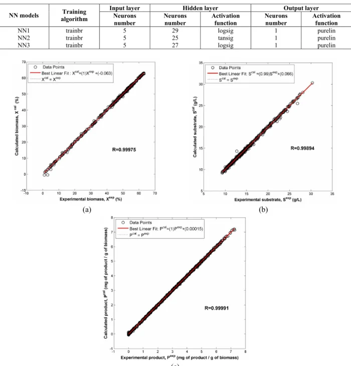
Table 3: Structure of the optimized NN models.
Input layer Hidden layer Output layer
NN models Training
algorithm Neurons number
Neurons number
Activation function
Neurons number
Activation function
NN1 trainbr 5 29 logsig 1 purelin NN2 trainbr 5 25 tansig 1 purelin NN3 trainbr 5 27 logsig 1 purelin
(a) (b)
(c)
From the optimized NN2, represented in Figure 3, we can express substrate uptake by a mathematical model that incorporates all inputs Ei (time, pH, RI, X0, S0) within it as follows:
The instance outputs Zj of the hidden layer:
5
I H
j H ji i j
i 1
5 5
I H I H
ji i j ji i j
i 1 i 1
5 5
I H I H
ji i j ji i j
i 1 i 1
Z f w E b
exp( w E b ) exp( w E b )
exp( w E b ) exp( w E b )
= = = = = ⎡ ⎤ = ⎢ + ⎥= ⎢ ⎥ ⎣ ⎦ + − − + + + − +
∑
∑
∑
∑
∑
(11)j=1, 2, … , 25
The output S:
25 25
H O H O
0 1j j 1 1j j 1
j 1 j 1
S f w Z b w Z b
= = ⎡ ⎤ ⎢ ⎥ = + = + ⎢ ⎥ ⎣
∑
⎦∑
(12)The combination of equations 11 and 12 leads to the mathematical formula for substrate uptake taking into account all the inputs Ei (time, pH, RI, X0, S0):
5
I H
ji i j i 1
5
I H
ji i j 25
H i 1 O
1j 5 1
j 1 I H
ji i j i 1
5
I H
ji i j i 1
exp w E b
exp w E b
S w b
exp w E b
exp w E b
= = = = = ⎡ ⎛ ⎞ ⎤ ⎢ ⎜⎜ + ⎟⎟ ⎥ ⎢ ⎝ ⎠ ⎥ ⎢ ⎛ ⎞⎥ ⎢− ⎜− + ⎟⎥ ⎜ ⎟ ⎢ ⎝ ⎠⎥ ⎢ ⎥ = ⎛ ⎞ + ⎢ ⎜ + ⎟ ⎥ ⎢ ⎜ ⎟ ⎥ ⎢ ⎝ ⎠ ⎥ ⎢ ⎛ ⎞⎥ ⎢+ ⎜⎜− + ⎟⎟⎥ ⎢ ⎝ ⎠⎥ ⎣ ⎦
∑
∑
∑
∑
∑
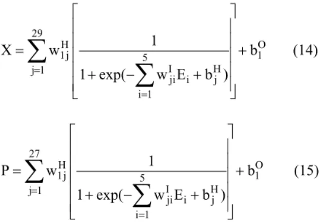
(13)Similarly, biomass and Pleuromutilin concentra-tions can be expressed by the mathematical
equations extracted from the optimized NN1 and NN3 as follows:
29
H O
1j 5 1
I H
j 1
ji i j i 1
1
X w b
1 exp( w E b )
= = ⎡ ⎤ ⎢ ⎥ ⎢ ⎥ = ⎢ ⎥+ ⎢ + − + ⎥ ⎢ ⎥ ⎣ ⎦
∑
∑
(14)27
H O
1j 5 1
I H
j 1
ji i j i 1
1
P w b
1 exp( w E b )
= = ⎡ ⎤ ⎢ ⎥ ⎢ ⎥ = ⎢ ⎥+ ⎢ + − + ⎥ ⎢ ⎥ ⎣ ⎦
∑
∑
(15)It is obvious that these FFNN mathematical equations for sugar uptake, biomass, and Pleuromutilin concentrations contain just the required degree of complexity, include the important relevant features that are operating conditions and initial conditions, and thus can readily be applied in control systems.
Comparison with Unstructured Kinetic Models
In order to establish the developed FFNN models as a plausible alternative to the unstructured kinetic models, a comparison between the two approaches was made in terms of simulation results, which is shown in Figure 4.
It is shown that the developed FFNN models outperform the unstructured kinetic models in predicting biomass, glucose, and Pleuromutilin concentration profiles.
The proposed forms of the specific rates of growth and product formation were suitable for some data sets and unsuitable for others. This is due to the behavior change of Pleurotus mutilus from one data set to another. This will probably require a change in the equations of the specific rates from one data set to another, thus making difficult their incorporation into a control-loop of the process.
(a)
(b)
(d)
Figure 4: Simulation results: (a) data set 2, (b) data set 4, (c) data set 9, (d) data set 17. (The experimental data (symbols) for biomass ( ), glucose ( ) and Pleuromutilin ( ); FFNN modeling results are represented by solid lines and kinetic modeling results are presented by long dashed lines)
Interpolation Performances
To check the accuracy of the three FFNN models previously developed and optimized, two types of interpolation databases were used. The first database contains a set of intermediate points between the experimental points of data set number 6, which was part of the learning and testing phases (data set number 6 was chosen randomly). The second data-base was two complete data sets never exploited during the learning and the test phases: (a) X0=4% and S0=26.6g/L; (b) X0=3% and S0=23.5g/L. The results of interpolation performances in terms of root
mean squared error (RMSE) and in terms of the correlation coefficient (R) are summarized in Table 4. The quality of fit of the first interpolation data set is depicted in Figure 5. An excellent fit to the experimental values of biomass, sugar and product can be noted.
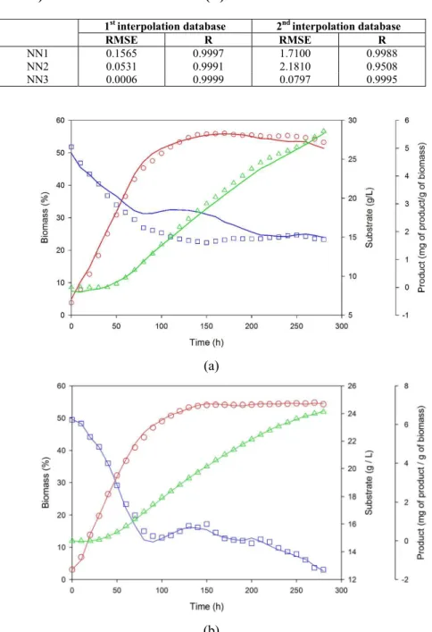
The modeling results of the second interpolation database derived from the three optimized FFNN models are plotted in Figure 6. It can be observed that both NN1 and NN3 were able to capture the process dynamics very well; however, NN2 results fitted only fairly the experimental glucose concentrations.
Table 4: Interpolation results in terms of root mean squared error (RMSE) and correlation coefficient (R).
1st interpolation database 2nd interpolation database
RMSE R RMSE R NN1 0.1565 0.9997 1.7100 0.9988 NN2 0.0531 0.9991 2.1810 0.9508 NN3 0.0006 0.9999 0.0797 0.9995
(a)
(b)
Figure 6: Simulation results of the second interpolation: (a) X0=4% and S0=26.6g/L; (b) X0=3% and S0=23.5g/L. (The interpolated experimental data (symbols) for biomass ( ), glucose ( ) and Pleuromutilin ( ); FFNN modeling results are represented by solid lines)
Although the accuracy of the FFNN models was moderately satisfactory, in particular for NN2, more historical data covering the whole field of interest should be added to the training phase in order to increase more and more the predictive quality of the FFNN models.
CONCLUSION
three feed-forward neural network models able to assess the three key bioprocess variables (biomass, substrate consumption and product) in the industrial fermentation of Pleuromutilin produced in a fed-batch mode. One of the more significant findings to emerge from this study is that, unlike the unstructured kinetic models, the optimized FFNN models could predict with enough accuracy the profiles of concentrations for all data sets.
In addition, mathematical formulae obtained from the optimized models not only include the important elements of the process, but they are also less complex, making their integration into an industrial control of the process easier.
However, artificial neural network modeling cannot replace kinetic modeling when trying to understand the phenomenon of fermentation.
REFERENCES
Asensio-Cuesta, S., Diego-Mas, J. A. and Alcaide-Marzal, J., Applying generalized feedforward neural networks to classifying industrial jobs in terms of risk of low back disorders. Int. J. Ind. Ergon., 40, 629-635 (2010).
Basheer, I. A. and Hajmeer, M., Artificial neural networks: Fundamentals, computing, design, and application. J. Microbiol. Methods, 43, 3-31 (2000).
Benkortbi, O., Hanini, S. and Bentahar, F., Batch kinetics and modelling of Pleuromutilin production by Pleurotus mutilis. Biochem. Eng. J., 36, 14-18 (2007).
Bishop, C. M., Neural Networks for Pattern Recognition. Oxford University Press (1995).
Bryjak, J., Ciesielski, K. and Zbicinski, I., Modelling of glucoamylase thermal inactivation in the presence of starch by artificial neural network. J. Biotechnol., 114, 177-185 (2004).
Cruz, A. J. G., Silva, A. S., Araujo, M. L. G. C., Giordano, R. C. and Hokka, C. O., Modelling and optimization of the cephalosporin C production bioprocess in a fed-batch bioreactor with invert sugar as substrate. Chem. Eng. Sci., 54, 3137-3142 (1999).
Cutlip, M. B. and Shacham, M., Problem Solving in Chemical and Biochemical Engineering with POLYMATH, Excel, and MATLAB. Prentice Hall (2008).
Danaher, S., Datta, S., Waddle, I. and Hackney, P., Erosion modelling using Bayesian regulated artificial neural networks. Wear, 256, 879-888 (2004).
Di Massimo, C., Montague, G. A., Willis, M. J., Tham, M. T. and Morris, A. J., Towards improved penicillin fermentation via artificial neural networks. Comput. Chem. Eng., 16, 283-291 (1992).
Egger, H. and Reinshagen, H., New pleuromutilin derivatives with enhanced antimicrobial activity I. Synthesis. J. Antibiot., 29, 915-922 (1976). Feyo de Azevedo, S., Dahm, B. and Oliveira, F. R.,
Hybrid modelling of biochemical processes: A comparison with the conventional approach. Comput. Chem. Eng., 21, 751-756 (1997).
Gevrey, M., Dimopoulos, I. and Lek, S., Review and comparison of methods to study the contribution of variables in artificial neural network models. Ecol. Modell., 160, 249-264 (2003).
Hagan, M. T., Demuth, H. B. and Beale, M. H., Neural Network Design. PWS Pub (1996).
Hannan, P. C. T., Windsor, H. M. and Ripley, P. H., In vitro susceptibilities of recent field isolates of Mycoplasma hyopneumoniae and Mycoplasma hyosynoviae to valnemulin (Econor®), tiamulin and enrofloxacin and the in vitro development of resistance to certain antimicrobial agents in Mycoplasma hyopneumoniae. Res. Vet. Sci., 63, 157-160 (1997).
Heaton, J., Introduction to Neural Networks with Java. Heaton Research, Inc. (2005).
Hirokawa, Y., Kinoshita, H., Tanaka, T., Nakamura, T., Fujimoto, K., Kashimoto, S., Kojima, T. and Kato, S., Pleuromutilin derivatives having a purine ring. Part 1: New compounds with promising antibacterial activity against resistant Gram-positive pathogens. Bioorg. Med. Chem. Lett., 18, 3556-3561 (2008).
Hirschen, K. and Schafer, M., Bayesian regulariza-tion neural networks for optimizing fluid flow processes. Comput. Meth. Appl. Mech. Eng., 195, 481-500 (2006).
Huang, J., Shimizu, H. and Shioya, S., Data pre-processing and output evaluation of an autoassociative neural network model for online fault detection in virginiamycin production. J. Biosci. Bioeng., 94, 70-77 (2002).
Kavanagh, F., Hervey, A. and Robbins, W. J., Antibiotic substances from basidiomycetes. VIII. Pleurotus mutilus and Pleurotus passeckerianus. Proc. Natl. Acad. Sci. U. S., 37, 570-574 (1951). Kovarova-Kovar, K., Gehlen, S., Kunze, A., Keller,
Laursen, S., Webb, D. and Ramirez, W. F., Dynamic hybrid neural network model of an industrial fed-batch fermentation process to produce foreign protein. Comput. Chem. Eng., 31, 163-170 (2007). Lee, D. S. and Park, J. M., Neural network modeling
for on-line estimation of nutrient dynamics in a sequentially-operated batch reactor. J. Biotechnol., 75, 229-239 (1999).
MacKay, D. J. C., Bayesian interpolation. Neural Comput., 4, 415-447 (1991).
Patnaik, P. R., Penicillin fermentation: Mechanisms and models for industrial-scale bioreactors. Crit. Rev. Microbiol., 27, 25-39 (2001).
Paul, G. C. and Thomas, C. R., A structured model for hyphal differentiation and penicillin production
using Penicillium chrysogenum. Biotechnol.
Bioeng., 51, 558-572 (1996).
Pigram, G. M. and MacDonald, T. R., Use of neural network models to predict industrial bioreactor effluent quality. Environ. Sci. Technol., 35, 157-162 (2000).
Pirt, S. J., Fed-Batch Culture of Microbes. Ann. N.Y. Acad. Sci., 326, 119-125 (1979).
Potocnik, P. and Grabec, I., Empirical modeling of antibiotic fermentation process using neural networks and genetic algorithms. Math. Comput. Simul., 49, 363-379 (1999).
Saraceno, A., Curcio, S., Calabro, V. and Iorio, G., A hybrid neural approach to model batch fermenta-tion of "ricotta cheese whey" to ethanol. Comput. Chem. Eng., 34, 1590-1596 (2009).
Shene, C., Diez, C. and Bravo, S., Neural networks for the prediction of the state of Zymomonas mobilis CP4 batch fermentations. Comput. Chem. Eng., 23, 1097-1108 (1999).
Si-Moussa, C., Hanini, S., Derriche, R., Bouhedda, M. and Bouzidi, A., Prediciton of high-pressure vapor liquid equilibrium of six binary systems, carbon dioxide with six esters, using an artificial neural network model. Braz. J. Chem. Eng., 25, 183-199 (2008).
Silva, J. A., Neto, E. H. C., Adriano, W. S., Ferreira, A. L. O. and Gonçalves, L. R.B., Use of neural networks in the mathematical modeling of the enzymic synthesis of amoxicillin catalysed by penicillin G acylase immobilized in chitosan. World J. Microbiol. Biotechnol., 24, 1761-1767 (2008).
Silva, R. G., Cruz, A. J. G., Hokka, C. O., Giordano, R. L. C. and Giordano, R. C., A hybrid feedforward neural network model for the cephalosporin C production process. Braz. J. Chem. Eng., 17, 587-598 (2000).
Stanbury, P. F., Whitaker, A. and Hall, S. J., Principles of Fermentation Technology. 2nd Ed. Butterworth-Heinemann (1999).
The Mathworks Inc.USA (2010).