FUNDAÇÃO GETULIO VARGAS
ESCOLA BRASILEIRA DE ADMINISTRAÇÃO PÚBLICA E DE EMPRESAS SETOR DE APOIO ACADÊMICO
CURSO DE MESTRADO ACADÊMICO EM GESTÃO DE EMPRESAS
VERSÃO PRELIMINAR DE DISSERTAÇÃO DE MESTRADO APRESENTADO POR
FELIPEBUCHBINDER
TÍTULO
THEBESTARENEVERNORMAL:
EXPLORINGTHEDISTRIBUTIONOFFIRMPERFORMANCE
PROFESSOR ORIENTADOR ACADÊMICO
RAFAELGOLDSZMIDT
V
ERSÃOP
RELIMINAR ACEITA,
DE ACORDO COM OP
ROJETO APROVADO EM:
DATA DA ACEITAÇÃO:______/_____/_____
FUNDAÇÃO GETÚLIO VARGAS
ESCOLA BRASILEIRA DE ADMINISTRAÇÃO PÚBLICA E DE EMPRESAS
THE BEST ARE NEVER NORMAL:
EXPLORING THE DISTRIBUTION OF FIRM PERFORMANCE
FELIPE BUCHBINDER
Dissertação apresentada à Fundação Getúlio Vargas-RJ – Escola Brasileira de Administração Pública e de Empresas, como requisito parcial à obtenção do título de Mestre em Administração.
Orientador: Professor Dr. Rafael Goldszmidt
FUNDAÇÃO GETÚLIO VARGAS
ESCOLA BRASILEIRA DE ADMINISTRAÇÃO PÚBLICA E DE EMPRESAS
THE BEST ARE NEVER NORMAL:
EXPLORING THE DISTRIBUTION OF FIRM PERFORMANCE
FELIPE BUCHBINDER
Este exemplar corresponde à versão final da dissertação defendida e aprovada pela Comissão Julgadora em 08/06/2011.
Banca Examinadora:
_______________________________
Prof. Dr. Rafael Goldszmidt – EBAPE/FGV
_______________________________
Prof. Dr. Flávio Carvalho de Vasconcelos – EBAPE/FGV
_______________________________
Prof. Dr. Luiz Artur Ledur Brito - EAESP/FGV
_______________________________
Prof. Dr. Jorge Ferreira da Silva - IAG/PUC
_______________________________
AGRADECIMENTOS
Há tantas pessoas a quem eu deveria agradecer que será impossível agradecer a
todas. Isto porque uma dissertação de mestrado não é um trabalho ao qual se chega
depois de meses de leitura e esforço, mas um rito de passagem que marca um momento
em uma trajetória muito mais ampla. Cada pessoa que, de alguma forma, me levou a
este trabalho contribuiu, de alguma maneira, para este momento. É certamente injusto
eu não citá-las todas, já que quem aprende de seu companheiro um único parágrafo,
uma única lei, um único versículo, uma única palavra ou mesmo uma única letra deveria
tratá-lo com respeito. Não sendo possível me lembrar de todos com quem eu já aprendi
alguma coisa, eu agradecerei aos mais recentes. Uma leitura sutil da dedicatória deste
trabalho mostrará ser ele dedicado a todas as pessoas citadas ou injustamente olvidadas
desta seção de agradecimentos.
Primeiramente, é preciso agradecer aos meus pais, Ricardo Buchbinder e Betina
Glejzer Buchbinder. De certa forma, este trabalho é deles já que, como me ensinou o
meu irmão, Gabriel Buchbinder, o que uma criança diz na rua são as palavras do seu pai
ou de sua mãe. Pensando nos meus pais, eu tenho a sensação de que este trabalho não
começou comigo e nem terminará no dia da defesa, mas que é uma modesta
contribuição minha localizada entre uma sucessão de gerações na História humana. Eu
espero que eu e meu irmão possamos realizar muitas outras contribuições neste sentido.
Quanto ao meu irmão, Gabriel Buchbinder, um único trabalho é homenagem
pouca. Ele que nunca pede nada, mas que sempre ajuda – e se preocupa em silêncio para
que a gente não saiba o quanto ele se importa – merece agradecimentos que não podem
ser expressos em palavras, mas apenas pelo amor fraterno e companheiro de uma vida
inteira. Que eu possa ter a felicidade de agradecê-lo como ele merece.
Agradeço em especial ao mestre e grande amigo Rafael Goldszmidt. As palavras
“mestre” e “amigo” não descrevem ninguém melhor. Havia um antigo costume dos
discípulos observarem o comportamento dos grandes sábios para aprenderem a conduzir
a vida cotidiana com modéstia e sabedoria. Eu faço o mesmo com o Rafael. Mais do que
Estatística ou Estratégia, eu aprendi com o Rafael o significado da expressão “sabedoria
de coração”. Por isso, enquanto a porta de sua sala estiver aberta, eu estarei
Agradeço ainda à Fundação Getulio Vargas, mais especificamente à EBAPE.
Depois de transitar como um estrangeiro entre Engenharia, Biologia, Física e o
mercado, é bom se sentir em casa.
Aos professores da EBAPE, graças aos quais meu mestrado foi uma época de
intenso aprendizado, tanto acerca da literatura existente em diversas áreas, quanto em
termos profissionais e pessoais. Um agradecimento especial aos professores Rafael
Goldszmidt, Flávio Carvalho Vasconcelos, Luiz Antônio Jóia, Ronaldo Parente,
Marcelo Milano Falcão Vieira, Henrique Guilherme Heidtmann Neto, Hélio Arthur
Reis Irigaray e à amiga de muitas conversas Mônica Pinhanez.
Aos meus colegas do MAGE. O que vivenciamos juntos não pode ser escrito!
Mas escrito está, espero, no coração e nas lembranças de cada um de nós. Eu nunca vi
um grupo tão unido e verdadeiramente amigo quanto a nossa turma. Eu ia feliz para as
aulas e a culpa é toda de vocês. Por essas experiências que nos acompanham na
memória, e pelas aventuras que nos aguardam no futuro, meus sinceros agradecimentos.
Os novos tempos, que trazem a turma do MAD e as que se seguirão, também são
bem-vindos. Dentro dele, como dentro de outros cursos na EBAPE, eu conheci amigos
com os quais troquei memoráveis conversas, conselhos e experiências. Espero lembrar
de todos com o decorrer dos anos, mas quero deixar registrado o nome de minha amiga
Carla Soares, por sempre ter um olhar mais sábio do que o meu sobre todas as coisas.
Aos funcionários da EBAPE, em especial ao Joarez Oliveira e à Celene Melo
pelo apoio e carinho de todas as horas durante o meu mestrado.
À Capes, pelo apoio financeiro essencial para o desenvolvimento desta
dissertação.
Agora que eu finalizo esta seção de agradecimentos - a última deste trabalho que
ora pareceu abençoadamente interminável - esta dissertação sai de minhas mãos e vai se
pousar diante dos olhos da banca e, espero, também diante dos olhos de outros leitores
curiosos. Que seja em uma boa hora e, se não for pedir muito, que possa trazer alguma
ABSTRACT
Competitive Strategy literature predicts three different mechanisms of performance generation, thus distinguishing between firms that have competitive advantage, firms that have competitive disadvantage or firms that have neither. Nonetheless, previous works in the field have fitted a single normal distribution to model firm performance. Here, we develop a new approach that distinguishes among performance generating mechanisms and allows the identification of firms with competitive advantage or disadvantage. Theorizing on the positive feedback loops by which firms with competitive advantage have facilitated access to acquire new resources, we proposed a distribution we believe data on firm performance should follow. We illustrate our model by assessing its fit to data on firm performance, addressing its theoretical implications and comparing it to previous works.
Keywords: Performance, Resource-Based View, Competitive advantage and
1
Table of Contents
1 INTRODUCTION ... 7
2 LITERATURE REVIEW ... 12
2.1 THE RBV FRAMEWORK AND ITS IMPLICATIONS ON PERFORMANCE DISTRIBUTION... 12
2.1.1 On the performance distribution for firms with competitive advantage or disadvantage ... 15
2.1.2 On the performance distribution for average performing firms ... 19
2.2 PREVIOUS WORKS ON THE OUTLIER PROBLEM IN STRATEGY RESEARCH ... 21
2.3 EXTREME VALUE THEORY AND COMPETITIVE ADVANTAGE AND DISADVANTAGE ... 23
2.4 BAYESIAN INFERENCE AND GIBBS SAMPLING ... 29
3 MODEL DEVELOPMENT ... 33
4 DATA ANALYSIS AND RESULTS ... 37
4.1 DATA AND VARIABLES ... 37
4.2 DISTRIBUTION FITTING ALGORITHM ... 40
4.3 RESULTS ... 41
4.3.1 Distribution fit ... 41
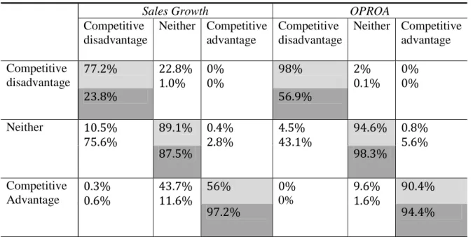
4.3.2 An exploratory assessment of whether the distribution’s portions are substantively different ... 48
4.3.3 Comparison with the results of an alternative approach ... 49
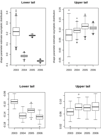
4.3.4 Evolution of performance distribution through time ... 52
5 CONCLUSIONS ... 60
5.1 LIMITATIONS ... 63
5.2 DIRECTIONS FOR FUTURE RESEARCH ... 65
6 REFERENCES ... 69
2
8 APPENDIX B ... 78
9 APPENDIX C ... 80
9.1 OPROA2003 ... 81
9.2 OPROA2004 ... 83
9.3 OPROA2005 ... 85
9.4 OPROA2006 ... 87
9.5 SALES GROWTH 2003–2004 ... 89
9.6 SALES GROWTH 2004–2005 ... 91
3
Table of Figures
FIGURE 1 – TUO APPROACHES FOR EXTREME VALUE THEORY. ... 23
FIGURE 2 - THE PROPOSED DISTRIBUTION FOR FIRM PERFORMANCE. ... 27
FIGURE 3 - THE HEAVISIDE STEP FUNCTION NOTATION... 34
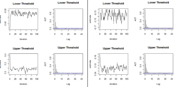
FIGURE 4 – CONVERGENCE HISTORY AND AUTOCORRELATIONS FOR AVERAGE SALES GROUTH AND OPROA. ... 42
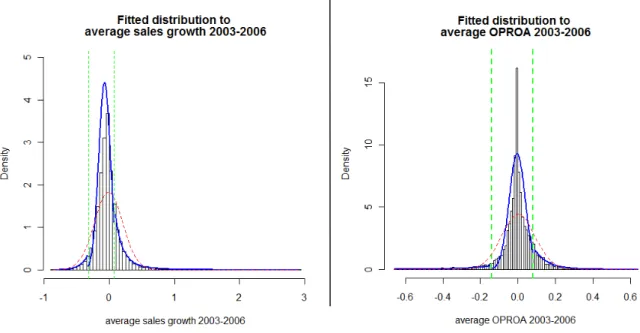
FIGURE 5 - FITTED DISTRIBUTION TO AVERAGE SALES GROUTH AND AVERAGE OPROA DATA. ... 44
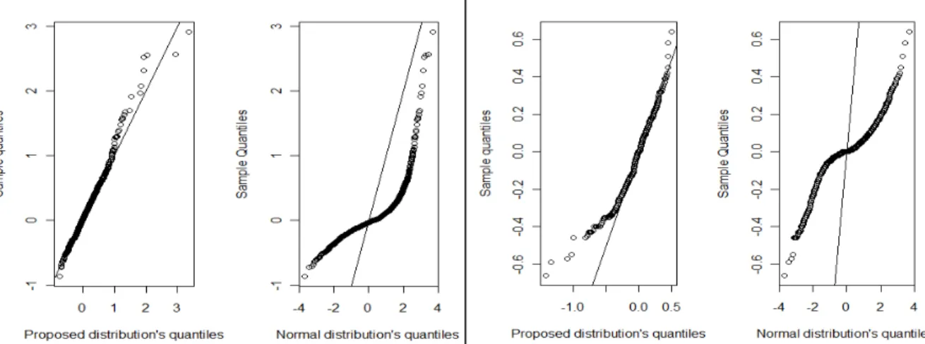
FIGURE 6 - QUANTILE PLOTS FOR AVERAGE SALES GROUTH AND OPROA. ... 46
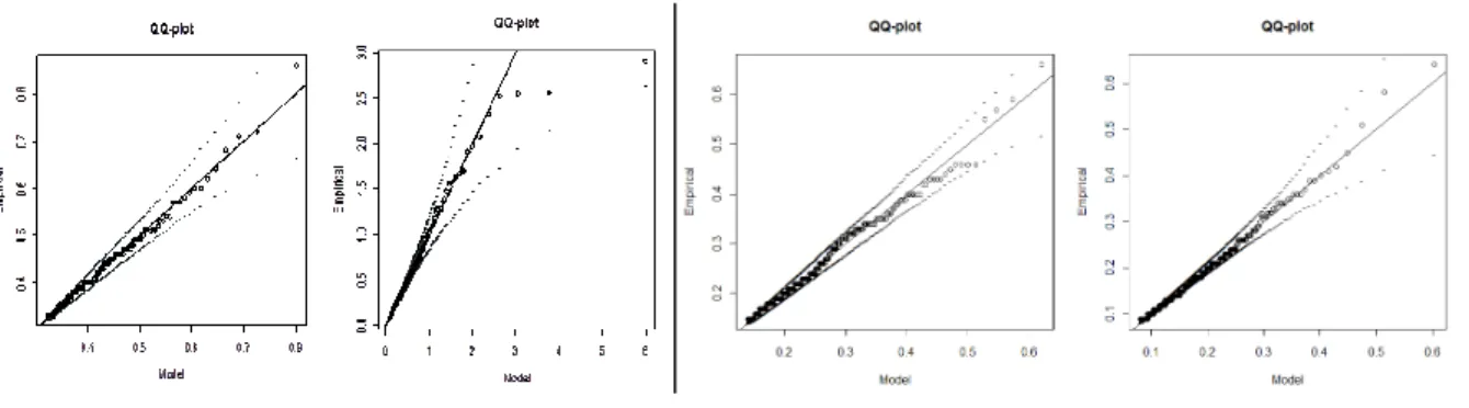
FIGURE 7 – QUANTILE PLOTS OF TAIL FIT TO AVERAGE SALES GROUTH AND OPROA DATA. ... 47
FIGURE 8 - PERFORMANCE DYNAMICS ... 57
FIGURE 9 - CONVERGENCE HISTORY AND AUTOCORRELATION FOR OPROA 2003. ... 81
FIGURE 10 - FITTED DISTRIBUTION TO CENTERED OPROA 2003 ... 81
FIGURE 11 - QUANTILE PLOTS FOR OPROA 2003. ... 82
FIGURE 12 - QUANTILE PLOTS OF TAILS FIT TO OPROA 2003 DATA. ... 82
FIGURE 13 - CONVERGENCE HISTORY AND AUTOCORRELATIONS FOR OPROA 2004. ... 83
FIGURE 14 - FITTED DISTRIBUTION TO CENTERED OPROA 2004. ... 83
FIGURE 15 - QUANTILE PLOTS FOR OPROA 2004. ... 84
FIGURE 16 - QUANTILE PLOTS OF TAILS FIT TO OPROA 2004 DATA. ... 84
FIGURE 17 - CONVERGENCE HISTORY AND AUTOCORRELATIONS FOR OPROA 2005. ... 85
FIGURE 18 - FITTED DISTRIBUTION TO CENTERED OPROA 2005. ... 85
FIGURE 19 - QUANTILE PLOTS FOR OPROA 2005. ... 86
FIGURE 20 - QUANTILE PLOTS OF TAILS FIT TO OPROA 2005 DATA. ... 86
FIGURE 21 - CONVERGENCE HISTORY AND AUTOCORRELATIONS FOR OPROA 2006. ... 87
FIGURE 22 - FITTED DISTRIBUTION TO CENTERED OPROA 2006. ... 87
FIGURE 23 - QUANTILE PLOTS FOR OPROA 2006. ... 88
4
FIGURE 25 - CONVERGENCE HISTORY AND AUTOCORRELATIONS FOR SALES GROUTH 2003-2004. ... 89
FIGURE 26 - FITTED DISTRIBUTION TO CENTERED SALES GROUTH 2003-2004. ... 89
FIGURE 27 - QUANTILE PLOTS FOR SALES GROUTH 2003-2004. ... 90
FIGURE 28 - QUANTILE PLOTS OF TAILS FIT TO SALES GROUTH 2003-2004 DATA. ... 90
FIGURE 29 - CONVERGENCE HISTORY AND AUTOCORRELATIONS FOR SALES GROUTH 2004-2005. ... 91
FIGURE 30 - FITTED DISTRIBUTION TO CENTERED SALES GROUTH 2004-2005. ... 91
FIGURE 31 - QUANTILE PLOTS FOR SALES GROUTH 2004-2005. ... 92
FIGURE 32 - QUANTILE PLOTS OF TAILS FIT TO SALES GROUTH 2004-2005 DATA. ... 92
FIGURE 33 - CONVERGENCE HISTORY AND AUTOCORRELATIONS FOR SALES GROUTH 2005-2006. ... 93
FIGURE 34 - FITTED DISTRIBUTION TO CENTERED SALES GROUTH 2005-2006. ... 93
FIGURE 35 - QUANTILE PLOTS FOR SALES GROUTH 2005-2006. ... 94
5
Table of Tables
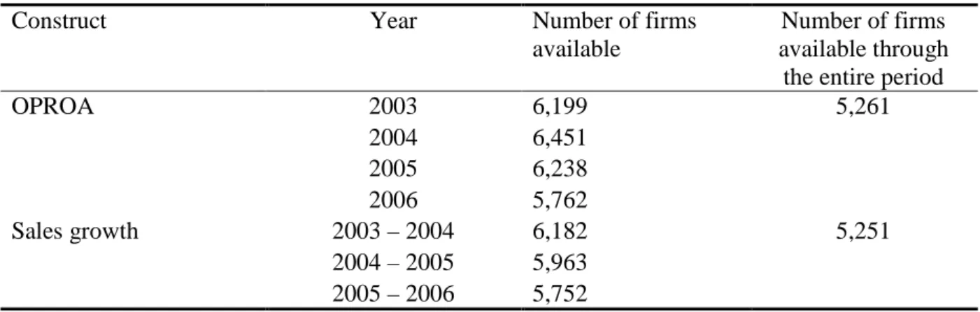
TABLE 1 - INFORMATION AVAILABLE PER INDICATOR AND PER YEAR ... 40
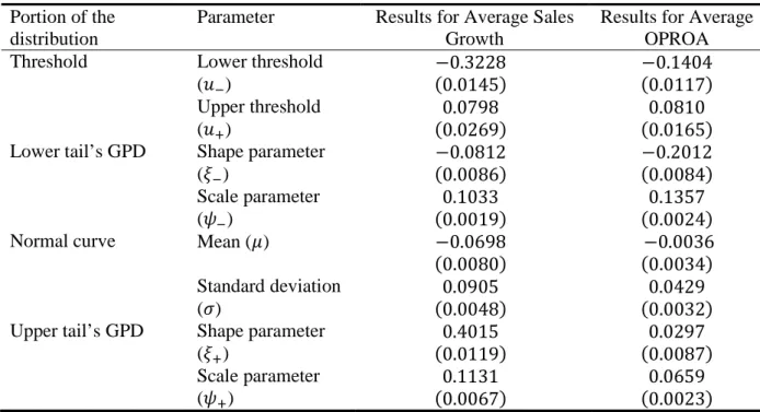
TABLE 2 - RESULTS FOR PARAMETER ESTIMATION ... 43
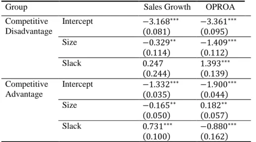
TABLE 3 –RESULTS FOR MULTINOMIAL LOGISTIC REGRESSION ... 49
TABLE 4 – COMPARISON UITH BRITO’S (2011) AND GOLDSZMIDT, BRITO AND VASCONCELOS’ (2011) METHOD ... 50
TABLE 5 - REPORT OF ABERRANT DATA EXCLUDED FROM THE COMPUSTAT DATABASE ... 76
TABLE 6 - ESTIMATED PARAMETER VALUES FOR DATA ON OPROA ... 80
6
Abbreviations
CLT - Central Limit Theorem
EB - Empirical Bayesian
EVT - Extreme Value Theory
GEV - Generalized Extreme Value
GPD - Generalized Pareto Distribution
IKS - Iterative Kolmogorov-Smirnov
OPROA - Operational return on assets
RBV - Resource-based view
ROA - Return on assets
7
1 Introduction
Competitive Strategy has grown to become a field of rich and lively debate among
different theories seeking to unveil the reasons why some firms attain exceptional performance
while others do not (Porter 1979; Barney, 1991; Peteraf, 1993; Rumelt, 1984; Teece, Pisano and
Shuen, 1997; Ghemawat, 2002; D'Aveni, Dagnino and Smith, 2010). Common to all these
theories is their reliance on the concepts of competitive advantage and superior performance.
Their pervasiveness notwithstanding, these concepts lack consensual definitions and there has
been some objection to the constructs used to measure them and to the methods by which the
firms that possess competitive advantage are identified (Chakravarthy, 1986; Wiggins and
Ruefli, 2002; Hansen, Perry and Reese, 2004; Combs, Crook and Shook, 2005; Hahn and Doh,
2006). This paper focuses on the least studied of the aforementioned issues, namely, the methods
used to identify firms which attain competitive advantage. Our research aims to fill this gap by
proposing a distribution by which firm performance may be modeled and wherefrom one may
identify those firms that have competitive advantage, competitive disadvantage or nothing but
average performance.
Competitive Strategy has evolved into becoming a field with matured theories
notwithstanding the ongoing debate on how are some of its key concepts to be defined, measured
and related to each other. Competitive advantage and performance are examples of such
concepts. Among the many definitions that have been given to competitive advantage, one finds
the ability of an organization to position itself well vis-à-vis its competitors (Williamson, 1991),
to create value (Porter, 1985) and to achieve above average returns (Peteraf, 1993). Similarly, the
8
numerous and imprecise and can be based on accounting measures, survival rates, growth,
shareholder value and hybrid constructs (Combs, Crook and Shook, 2005). Such multiplicity in
definitions shows that the concepts of organizational performance and competitive advantage, in
spite of their omnipresence throughout Competitive Strategy literature, lack consensual
definitions (Chakravarthy, 1986; Combs, Crook and Shook, 2005).
In addition, the relationship between competitive advantage and superior performance
has been deemed by some authors a logical fallacy (Coff, 1999; Powell, 2001; Arend, 2003;
Tang and Liou, 2010), insofar as researchers “infer the existence of competitive advantage from
ex post superior performance, and conclude that creating competitive advantages ex ante will
produce superior performance” (Tang and Liou, 2010:41-42). Coff (1999), Powell (2001) and
Tang and Liou (2010) go as far as noting that competitive advantage need not necessarily lead to
superior performance. Thus, equally multiple as the definitions of competitive advantage and
firm performance are the causality relationships by which these two concepts are theoretically
connected (Powell, 2001; Durand, 2002; Durand and Vaara, 2009; Tang and Liou, 2010).
Amidst such criticism are the challenging tasks to identify and study those firms that truly
achieve sustained superior performance. Such difficulties have been previously noted by
Wiggins and Ruefli (2002; 2005), Hansen, Perry and Reese (2004) and Hahn and Doh (2006)
and lie in the fact that the firms that most interest researchers in the field of Strategy are outliers,
insofar as their performance is considerably above (or below) average by definition. Most
statistical techniques, however, stem from the central limit theorem and are very sensible to
outliers. This leads many researchers to exclude outliers from their datasets but, in doing so, they
are excluding data in some of those firms that matter the most (Wiggins and Ruefli, 2002;
9
firm heterogeneity, such as the resource-based view (Barney, 1991), since statistical techniques
that focus on means and averages are incapable of any assessment of firm uniqueness (Hansen,
Perry and Reese, 2004).
Since Competitive Strategy is an applied domain of knowledge, both researchers and
practitioners must be able to assess the empirical validity of its theoretical frameworks. Such
assessment requires, nonetheless, that researchers be equipped with appropriate tools to handle
the challenges it presents, even if this means having to draw statistical inferences from outlier
data.
This paper aims to contribute to strategy research by proposing a method by which firms
with competitive advantage and disadvantage may be identified. In order to do so, we draw from
the resource-based view (RBV) of the firm and argue that there is an inconsistency between
theory and the empirical approaches so far employed to assess this theory. Such inconsistency
lies in the fact that, while theory acknowledges that there are different underlying mechanisms
generating performance in firms with competitive advantage, competitive disadvantage or
neither, empirical studies fit a single distribution to model performance data. A single
distribution, however, implies that there is a single mechanism generating performance in all
firms, albeit with different degrees. Nonetheless, competitive disadvantage is not a lesser degree
of competitive advantage, but something entirely different (Tang and Liou, 2010) and, therefore,
each must be modeled by a distribution of its own. However, we know of no paper who has
considered such approach previously.
In this paper, we shall not attempt to resolve the entire philosophical discussion revolving
around the concepts of competitive advantage and organizational performance. Rather, we shall
10
employed so far in Competitive Strategy empirical studies (Combs, Crook and Shook, 2005) and
that a causal relationship does exist between competitive advantage and organizational
performance. If future researchers come to find that current measures of performance are indeed
inadequate, our method should still be valid and may be appropriately changed if necessary.
Henceforth, we focus solely on the outlier problem, namely, how they can be detected in
empirical studies in the field of strategy.
In the next section, we review the RBV framework and show how it requires
organizational performance to follow a peculiar distribution. This shall motivate us to propose
that performance does indeed obey such a distribution. This distribution shall allow different
performance generating mechanisms for firms with competitive advantage and disadvantage, as
well as include those firms that would be excluded as outliers in conventional models and,
therefore, it is the major theoretical outcome of this paper. Methodologically, however, we shall
note that current techniques are unable to fit the proposed distribution to data. Seeking to resolve
this issue, we then make a literature review on previous works on the field of Strategy that have
considered the outlier dilemma. We will note two separate calls for greater use of Bayesian
inference and Extreme Value theory. We will follow these advices and show that they are
sufficient to develop a method by which the proposed distribution may be fitted to actual data. In
order to do so, each of these fields of knowledge will be presented, though only to the extent to
which it is necessary for the comprehension of the method we hereby propose.
The following section contains the model development, after which two sections
elaborate on the methodological approaches to treat the data and present the results obtained after
applying the proposed model to empirical observations. The two last sections discuss the results
11
strengths and caveats of the method that has been proposed and the results that have been shown
12
2 Literature Review
In this section, we briefly review existing literature on the RBV of the firm and argue
how it requires that data on performance adhere to a certain distribution. Then, we review
previous literature on the outlier problem in the field of Competitive Strategy and the
propositions that have been made in order to address this issue. We choose to develop our own
proposition by combining Extreme Value Theory and Bayesian inference and showing that the
same distribution we had derived on a RBV context is able to resolve the outlier problem
regardless of the mechanisms generating firm performance. To this end, we present the aspects
of these theories that shall be useful for our model’s development in the next section.
2.1 The RBV framework and its implications on performance distribution
According to Makadok (2010), there are four basic causal mechanisms by which scholars
in Strategy and Economics have sought to explain performance: competitive advantage, rivalry
restraint, information asymmetry and commitment timing. The RBV believes that performance is
causally related to competitive advantage and that the latter stems from the firm’s possession of
certain kinds of resources (Wernerfelt, 1984; Barney, 1991; Rumelt, 1991; Peteraf, 1993,
Wernerfelt, 1995). In a nutshell, the RBV holds that the fundamental determinants of firm
performance lie within the firm itself (Wernerfelt, 1984). These ultimate causes of firm
performance are called resources and, in order for them to confer sustained competitive
advantages, they must be valuable (lest they should be useless), rare (lest others should have
them), imperfectly mobile (lest others should acquire them) and non-substitutable (lest others
13
resources often exhibit complex interactions among themselves, leading to different phenomena
such as causal ambiguity (Rumelt, 1984; Reed and DeFillipi, 1990), path dependence (Dierickx
and Cool, 1989) and, ultimately, to competitive advantage itself (Rumelt, 1984; Wernerfelt,
1984; Barney, 1991).
Not all firms, however, possess competitive advantage (Rumelt, 1984; Barney, 1991).
Since sustained ricardian rents are ultimately a consequence of resource possession and their
interactions, the mechanisms generating firm performance ought to be different in the presence
or in the absence of such resources. With different mechanisms generating performance in firms
with or without competitive advantage, however, it stands to reason that performance of such
firms will follow different distributions. Therefore, it is reasonable to expect that data on
performance will not adhere to any single distribution but, rather, that a distribution with
different parts will be necessary to fit such data. The question remains as to how many parts will
be necessary.
The RBV is quite straightforward in distinguishing two kinds of firms, namely, those that
have and those that lack competitive advantage (Barney, 1991). As the theory matured, it became
evident that competitive advantage had a nemesis. Just as some firms had the gift of being
endowed with resources that granted them competitive advantage, some other firms had to carry
the unfortunate burden of resources that forced them into a situation of competitive disadvantage
(Powell, 2001; Brito and Vasconcelos, 2004; Tang and Liou, 2010). Thus, competitive
disadvantage appeared as a third alternative besides competitive advantage and lack thereof. The
existence of three distinct types of firm suggests that performance data should be composed of
14
asked: what is a distribution? Or, alternatively, under what theoretical grounds can one state that
something follows a given distribution?
Classical probability theory describes phenomena by associating to each phenomenon a
random variable. In each observation of the phenomenon, the random variable assumes a specific
value which is generated by a certain mechanism, expressed mathematically as the random
variable’s density function, or distribution (Goldberger, 1991). Hence, one speaks ultimately of a
mechanism that generates data values and, ultimately, a distribution. Thus, a distribution is the
mathematical expression of a mechanism that generates data in a certain way. A corollary to this
proposition is that different mechanisms must be associated with different distributions.
Extant literature in the RBV perspective refers to three different mechanisms to generate
performance. Thus, when a firm possesses valuable, rare, imperfectly mobile and
non-substitutable resources, its performance cannot be accounted for in the same way as the
performance of a firm which lacks such resources, insofar as one derives ricardian rents while
the other is subject to the laws of classical economics theory which prevents economic profit to
be sustained (Makadok, 2010). This comparison illustrates that there are different mechanisms
that generate performance in either case. A similar argument may be given to show how
performance in firms with competitive disadvantage is generated by yet another mechanism,
totalizing three distinct performance generating mechanisms predicted by the RBV framework.
Since each mechanism corresponds, in classical probability theory, to a single distribution, it
follows that three mechanisms ought to be described by three distinct distributions.
The previous paragraphs have shown how fitting a single distribution to performance data
15
question remains as to the exact forms of these distributions. This will require some investigation
on resource interdependence, which is done on the following paragraphs.
2.1.1 On the performance distribution for firms with competitive advantage or disadvantage
In the RBV framework, a firm is said to be a “bundle of resources” (Wernerfelt, 1984). It is from
the joint effects of these resources that competitive advantage emerges. Sustained competitive
advantage, rather than being the consequence of the possession of a single resource, often
requires multiple resources that combine in order to grant exclusiveness to ricardian rents.
Therefore, resources, far from being independent, are powerfully interrelated and interdependent.
One resource depends on other resources to derives its attributes of value, rareness, imperfect
mobility and non-substitutability, so positive feedback mechanisms by which the firm’s ability to
generate competitive advantage is enhanced. Causal ambiguity, for instance, is a notorious
example of how different resources interact to create imperfect mobility and, ultimately,
establish the sustainability of a firm’s ricardian rents (Dierickx and Cool, 1989). Resource
interdependence is also evident in the fact that the possession of certain resources has been
shown to make it easier for firms to acquire more of the same resources (Teece, Pisano and
Shuen, 1997) as well as resources of another kind (Wernerfelt, 2010). Indeed, the feedback
mechanisms that originate from resource interaction have been argued by Vergne and Durand
(2011) to eventually lead to path dependence and, therefore, to establish an asymmetry among
the efforts firms have to undertake in order to acquire new resources.
Consider, as a hypothetical illustration, a firm whose brand is admired by consumers at
16
government, thus using one already valuable resource to acquire another valuable resource.
Contacts with government might give the firm access to exclusive information and maybe make
it a first mover when such a move seems profitable. Workers of a first mover firm with a
renowned brand are likely to be more easily motivated and put more effort and quality in their
work, making the firm more efficient. But with happy workers, the firm might become
acknowledged as one of the “top 100 places to work at”, thus making brand name even stronger
and giving the firm access to more qualified employees.
Though this is a theoretical example, it illustrates how the possession of specific
resources leads to the possession of other resources in a continuous generation of ricardian rents.
A rival firm, watching this dynamics from the outside, will be unable to pinpoint the exact
resource that accounts for our firm’s exceptional returns, as a consequence of path dependence
and casual ambiguity. Hence, the possession of certain resources trigger feedback loops by
which new resources may be acquired to enhance performance and to prevent the resources
themselves from being imitated. A curious example of how such feedback loops may generate a
continuous path-dependent sequence of resource acquisition is Nokia, a telecommunications
company which began as paper producer about 150 years ago (Behr, 2001; Brown-Humes and
Skapinaker, 2001).
The graphical representation of this phenomenon on a histogram would be the thus: the
block that represents the firm at hand would move away from the mean in the direction of the
positive axis, gradually becoming an ever more extreme observation and, ultimately, an outlier.
When such phenomenon happens to a number of firms, their movement towards the positive axis
causes the histogram’s upper tail to fatten, thus accounting for performance distribution’s
17
In more formal terms, the RBV literature posits that resources are convolutely
intertwined and interdependent, with different resources mutually moderating each other,
particularly via positive feedback mechanisms that augment their impact on firm performance
(Vergne and Durand, 2011). Phenomena that exhibit a high degree of interdependence between
its occurrences, particularly when positive feedback loops are present, are consistently described
by a Generalized Pareto Distribution (GPD) (McKelvey and Andriani, 2005; 2007; 2009). The
reason for this is that the feedback loops increase the intensity of the observed phenomenon,
driving it farther from average. As a consequence, extreme observations become more frequent
than normal and a heavy-tailed distribution arises.
The GPD is the general form of one-sided heavy-tailed distributions and, therefore, it is
precisely the distribution being described here. Such distribution is therefore a reasonable choice
to model the performance of firms that have competitive advantage. As the matter of fact,
McKelvey and Andriani (2009) list 80 phenomena extracted from social sciences that have been
previously proven to follow a GPD. Therefore, though we know no instance when the GPD has
been previously employed in the field of Competitive Strategy, it has been successfully
employed in many phenomena from neighboring disciplines. Hence, incorporating the GPD into
our model is not only a choice that is consistent with theory, but a choice that has been
empirically verified in many other phenomena where interdependencies and positive feedback
loops are present.
Indeed, the theory underlying such phenomena was addressed by Herbert Simon (1955)
18
of preferential attachment1. Hence, the ease of firms which possess certain resources to acquire
other resources is but a manifestation of preferential attachment in the RBV framework.
Metaphorically, one might visualize resources “attaching” themselves to preexisting bundle of
resources (i.e. firms) with higher probability the more resources are available in each bundle.
Quite consistently, Herbert Simon (1955) has also found that preferential attachment leads to the
emergence of heavy tails which, in turn, can be described by a GPD.
An unrealistic consequence of our argument and of Herbert Simon’s preferential
attachment, however, is that observations become ever more extremes in an unending fattening
of the tails. In the real world, however, abrupt changes do occur and even mighty firms may go
bankrupt. Preferential attachment does not account for this but an explanation can be given under
the RBV framework. Goldszmidt (2010) suggests that, under periods of crisis, resources that
conferred competitive advantage may cease to do so, whereas other resources may become
valuable and able to generate ricardian rents. Hence, under a crisis, firms that were previously
competitive may find their resources to be of no avail, and firms that had resources of little value
may find them useful to profit from changing times. As a consequence, extreme observations
should move closer to the average and the heavy tails should become thinner.
Indeed, changes in resources’ values may occur in spite of crisis as a resource spans its
lifecycle (Helfat and Peteraf, 2003) or as the industry matures (Miller and Shamsie, 1996).
19
Observing such phenomena is no easy task, since the value of a resource is often a latent
variable, not to mention the stage of its lifecycle wherein it is. In addition, at any given time,
different resources may be in different stages of their respective lifecycles, so it is not clear how
their effects combine to halt tail thickening, nor if they do halt tail thickening at all. In the
example studied by Miller and Shamsie (1996), for instance, though there is change in resources’
values, this was not accompanied by a loss of competitive advantage in Hollywood’s movie
industry. Thus, though changes in resources’ values may hinder preferential attachment, halt tail
thickening and promote tail retraction, the circumstances under which this happens are not yet
fully understood. Economic crisis, however, are a noteworthy example of circumstances where
changes in resources’ values do hinder firm performance and which is peculiarly suited for
empirical research due to its observable character (Latham & Braun, 2008; Goldszmidt, 2010;
Gulati, Nohria & Wohlgezogen 2010).
Though the previous paragraphs presented arguments related to firms with competitive
advantage, the same conclusions should hold for firms with competitive disadvantage,
whereupon data on such firms’ performance should also adhere to a GPD. A noteworthy
difference between both tails, however, is that whereas firms might endure with endlessly
increasing performance, firms which incur in repeated losses are unlikely to last long. Hence, the
lower tail differs from the upper tail by the existence of a survival bias. As a consequence of this
bias, the lower tail is likely to be shorter and less populated than the upper tail.
2.1.2 On the performance distribution for average performing firms
The question remains as to which distribution should model performance of those firms
20
as there are resources that can confer a firm competitive advantage, there are other resources that
can account for competitive disadvantage, as well as resources that result in neither. In the
bundle of resources that constitutes a firm, one should find resources of all types. Tang and Liou
(2010) theorize that it’s the sum of the effects of these resources that will result in competitive
advantage, if valuable resources outweigh their counterparts, or in competitive disadvantage, if
otherwise. What should happen if one kind of resource only barely outweighs the other? One
might argue that if “positive” and “negative” resources barely cancel each other, the remaining
sum of their effects is not sufficient to generate the positive feedback loop required to drive them
to the tails of the distribution. Stated otherwise, perhaps a firm must have a minimum excess of
“positive” over “negative” resources in order to generate competitive advantage. If a firm is
incapable of reaching this minimum excess, the resources a firm possesses will be of little avail
to help it acquire more resources, so the positive feedback loops that drives some firms to a GPD
cannot work on them.
According to McKelvey and Andriani (2005; 2007; 2009), while GPD emerges in
phenomena where self-reinforcing mechanisms in some observations drives them continuously
away from the mean, phenomena in social sciences in which such mechanisms are not present
are normally distributed. Therefore, data on performance of firms with neither competitive
advantage nor disadvantage is expected to adhere to a normal distribution (McKelvey and
Andriani, 2005; 2007; 2009). This is indeed consistent with the normal allure which is
empirically found in histograms of performance data.
Hence, drawing from the RBV framework, we hold that data on firm performance should
be described by three distinct distributions: (1) a GPD for firms with competitive advantage; (2)
21
performing firms, with lack both competitive advantage and disadvantage. Though the
discussions presented so far yield a theoretical contribution to Competitive Strategy literature,
this contribution is of little practical avail, given that we lack the method by which the
aforementioned distributions may be jointly fitted to real data. In order to develop such method,
however, we will draw inspiration from previous works on the outlier problem and their call for
a greater use of two mathematical tools, namely, EVT and Bayesian Inference. We will show
that these tools shall enable us to develop the model we seek and, in doing so, it will become
evident that, the same distributions we proposed using arguments derived from the RBV
framework might be derived using solely mathematical considerations. In order to do so, we will
seek to derive anew the same conclusions we arrived at in this section.
2.2 Previous works on the outlier problem in Strategy research
Many fields of knowledge have struggled with the challenge to deal with outliers (e.g.
Fama, 1965; Clark, 1989; De Giuli, Maggi and Tarantola, 2010) and their exclusion has been a
common practice at least ever since Bernoulli advised it in 1771 (Collet and Lewis, 1976; Clark,
1989). It is nonetheless surprising that strategy researchers have shown little concern with outlier
exclusion, despite the fact that the most interesting examples of successful strategy are outliers
themselves. To the best of our knowledge, Wiggins and Ruefli (2002), Hansen, Perry and Reese
(2004) and Hahn and Doh (2006) are notable exceptions. In the following paragraphs, we briefly
review their proposals to dealing with the outlier problem.
Wiggins and Ruefli (2002) detect outliers by a method called the Iterative
Smirnov (IKS) approach. This method consists on sequentially applying the
22
potential stratum cumulative distribution. When all iterations have been made, the IKS approach
allows data to be divided into different strata, as explained in Wiggins and Ruefli (2002) and in
greater detail in Wiggins and Ruefli (2000). The authors argue that one of the main advantages
of this method is that it does not require a previously determined number of strata. In practice
however, since the IKS approach may lead to single observation strata, Wiggins and Ruefli
(2002) limited strata number to three. Our approach shall establish outright the existence of three
strata, but such choice is grounded in theoretical reasons, as we will further explain.
Hansen, Perry and Reese (2004) and Hahn and Doh (2006) suggest the field of strategy
would greatly benefit from incorporating Bayesian inference’s techniques, among whose
advantages lies the ability to incorporate outlier information. Other advantages of the use of
Bayesian inference is the ability to deal with small samples, which is especially useful for studies
focusing on the outliers themselves.
We follow the advice of Hansen, Perry and Reese (2004) and Hahn and Doh (2006) and
build our model on a Bayesian framework. In so doing, we draw a philosophical difference
between Wiggin and Ruefli’s (2002) method and ours, insofar as their approach is frequentist
and ours Bayesian. Additionally, we incorporated the merits of Bayesian inference, as taught by
Hansen, Perry and Reese (2004) and Hahn and Doh (2006) and reviewed shortly.
In addition, we also consider the call of McKelvey and Andriani (2005) and Nystrom,
Soofi and Yasai-Ardekani (2010) for a more widespread use of Extreme Value Theory (EVT) in
Management Sciences. Since outliers are nothing short of extreme events, we find it useful to
learn from both Bayesian inference and Extreme value theory in order to tackle the outlier
problem. In the following sessions, we briefly present the topics of either theory that shall be
2.3 Extreme value theory
When studying averag
mean will approximately follo
such as outliers, the CLT is n
sample extremes. Extreme Va
depends, indeed, in how is the
EVT literature has con
observations are extremes or
divides data into blocks and c
Tippet, 1928; Gumbel, 1935
observations are deemed extre
Figure 1, where extreme distrib
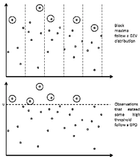
Figure 1 – Two approaches for Extrem
Note: Above, block maxima are deemed exceed some high threshold. In either ca value (GEV) distribution, while peaks ov extremes that shall be used in this paper.
23
ory and competitive advantage and disad
rage phenomena, the central limit theorem (CL
llow a normal distribution. When dealing with
s not applicable and a new distribution is need
Value Theory (EVT) studies which distributio
he word “extreme” to be defined (Coles, 2004;
onsolidated two equally accepted approaches fo
or not (McNeil, 1997; Coles, 2004; Bali, 2007
d considers the maximum of each block to be
35). The other approach establishes a thresh
treme (Pickands, 1975). Both definitions are sc
tributions are emphasized by being circumscrib
reme Value Theory.
ed extreme observations, whereas below, extreme observation case, extreme observations are circumscribed. Block maxima f
over threshold follow a generalized Pareto distribution (GPD) er.
sadvantage
CLT) assures us sample
ith extreme phenomena,
eeded in order to model
tion this is. The answer
; Bali, 2007).
s for classifying whether
007). The first approach
be extreme (Fisher and
eshold above which all
schematically shown in
ribed
24
Whereas Nystrom, Soofi and Yasai-Ardekani (2010) used the first of the aforementioned
approaches, it is the second one that shall be adopted in this work’s empirical analysis, since an
outlier is nothing short of an observation that exceeds a threshold too high (or too low) not to
draw attention to itself2. Henceforth, we shall use the word “extreme” only in this context.
Moreover, we shall present the EVT for extremes that surpass some high threshold. Extremes
that plunge below some low threshold can be dealt with by changing the sign of every element in
the sample (Coles, 2004).
In classical probability theory, the probability law that describes the behavior of data
, , … generated from a parent distribution whose cumulative distribution function is given by
over some threshold is:
| 1 1 0 (1)
More often than not, however, we are ignorant on the nature of the parent distribution
(McNeil, 1997; Coles, 2004). Fortunately, the Pickands-Balkema-de Haan (PBH) theorem states
that, for a very large class of parent distributions, | converges, as the
2
25
threshold grows large, to a distribution known as the Generalized Pareto Distribution (GPD)
(Balkema, de Haan, 1974; Pickands, 1975). In more mathematical terms:
lim | 1
Where
1 1 ! /# (2)
is the GPD written in terms of the threshold excess, $. To write it in terms of the original
variable , it would suffice to substitute % . In particular, for 0, the GPD
becomes an exponential distribution with parameter ! . The formula is defined for & | 0 '
1 / 0(. Here, ) * is called a shape parameter whereas 0 is termed a scale
parameter (McNeil, 1997; Coles, 2004; Bali, 2007). Intuitively, can be thought of as the weight
of the parent distribution’s tails and is therefore related to this distribution’s kurtosis. Thus, it
measures how frequent extreme observations are in the underlying process that generates the
observed data (McNeil, 1997; Coles, 2004). The scale parameter , however, has a less intuitive
interpretation. Equation (2) may be written in terms of +
,!-. /, which bears resemblance to the
normal’s +,!0
1 / and is likewise called a standardized form. Additionally, both and the standard
deviation are called scale parameters. Identifying and 2, however, is an erroneous
interpretation, since is not the square root of the GPD’s variance. A preferable interpretation is
that 1/ is the value of the GPD’s density function at the threshold, which can be proved by
taking the derivative of equation (2). Nonetheless, this interpretation says little on the role of the
26
interpretation, therefore, is not straightforward and it is better to think of it in abstract terms
(Coles, 2004).
Other than modeling extreme events, it stems from equation (1) that the GPD can also be
used to model parent distribution tails. This is a feature of the PBH theorem that is not found in
the CLT, since the CLT cannot guarantee that the parent distribution function be approximated
by a normal curve in the vicinities of the expected value. As far as the parent distribution tails are
concerned, however, the PBH theorem states that they can be approximated by a GPD. Indeed,
equation (1) may be written
31 4 5 |
Since 5 | may be approximated by a GPD for sufficiently high thresholds, it
can be shown that the tails of will also asymptotically follow a GPD (Pickands, 1975;
McNeil, 1997; Bali, 2007). This will be of interest in our model.
Since the GPD can be used to model tails (Pickands, 1975; McNeil, 1997; Bali, 2007)
and previous empirical research has shown average performance data to have a normal allure, it
follows that any reasonably typical parent distribution of firm performance may therefore be
expressed, as depicted in Figure 2, as a combination of three distinct distributions: (1) a GPD for
exceptionally well performing firms; (2) a normal curve for those firms who perform on average
and (3) another GPD for those ill-performing firms who nonetheless, manage to survive
somehow. Indeed, since performance distributions have two tails (each of which is predicted by
the PBH theorem to asymptotically follow a GPD) and a central portion (which one has no a
priori reason to divide in smaller portions), the number three emerges naturally as the number of
portions of performance distribution. Though this is a purely mathematical argument for why
arguments previously develop
distribution. Thus, this threefo
but from both. A couple of com
Figure 2 - The proposed distribution f
Note: The distribution is composed of th and right tail, respectively. The two tails justified by the tail-fitting property of leptokurtosis in firm performance distrib
First, it is interesting t
the distribution we had previou
only that this time solely mat
into distributions (1), (2) and (
to have competitive advantag
competitive disadvantage, resp
Liou, 2010). It follows that co
the sheer lack of any sort of co
success requirements”. Indee
parameters, one is assured th
(Powell, 2001; Tang and Liou,
27
oped under the RBV framework, which arrived
efold division stems neither from mathematics n
comments can be derived from this.
n for firm performance.
f three regions: a normal curve in its center, and a GDP for m ils correspond to firms with competitive advantage and disadv of the PBH theorem. Since the GPD is heavy-tailed, the ribution. Note that the distribution need not be symmetrical.
g to note that the distribution currently under s
iously arrived at using arguments derived from
athematical arguments were used. Specificall
d (3) are those firms that, Competitive Strategy
age (Barney, 1991), to have no competitive a
respectively (Powell, 2001; Brito and Vasconc
competitive disadvantage, as predicted by Pow
f competitive advantage, but “the failure even to
eed, since distributions (1) and (3) have di
that competitive advantage and disadvantage
ou, 2010).
ed at precisely the same
s nor from theory alone,
r minima and maxima on its left dvantage and their GPD form is their use allows to incorporate
er study is no other than
om the RBV framework,
ally, those firms that fit
egy theory would predict
e advantage and to have
ncelos, 2004; Tang and
owell (2001:881), is not
n to satisfy the minimum
different and unrelated
28
In addition, the fact that data on performance is found ubiquitously to be somewhat
leptokurtic suggests that the tails of firm performance distribution are not normal (Mandelbrot,
1963; Fama, 1965; McKelvey and Andriani, 2005). This hints at the fact that one should, in fact,
distinguish between the center and the tails of performance distributions and not treat
distributions (1) and (3) as mere continuations of distribution (2), but rather as distributions of
another kind. Additionally, the law of Pareto-Lévy states that all stable distributions besides the
normal curve are heavy-tailed (Fama, 1963; Mandelbrot, 1963; Fama, 1965; Mantegna and
Stanley, 2000), thus assuring that the GPD, which is itself a stable distribution, is theoretically
suited for the modeling of leptokurtic phenomena such as ours.
Finally, this section has drawn on knowledge from EVT to propose a theoretical
distribution to fit data on firm performance. Insofar as the arguments employed stemmed from a
mathematical theorem, they are not limited to any theory on the origin of firm performance.
Thus, our model is not confined to the RBV or to any other theory in Strategy. Rather, it
precedes those theories, inasmuch as it proposes to fit data on performance regardless on the
underling generating mechanisms that generate such data.
Though there is no algebraic solution to the maximum likelihood estimates of the GPD
parameters (Coles, 2004; Bali, 2007), some estimators have been proposed (Hill, 1975) and
curve fitting can be made by computational methods (Coles, 2004; Bali, 2007). Nonetheless,
whereas it is possible to estimate and , estimating the threshold above which observations are
deemed extreme is often very challenging. Traditionally, threshold choice relied on graphs
whose interpretation is frequently very difficult and highly subjective (for an overview of these
29
estimating and by conventional log-likelihood maximization computational methods (Coles,
2004; Bali, 2007).
In the next session, we review those aspects of Bayesian inference that shall be relevant
in our method, as well as the computational techniques that shall be used for parameter
estimation.
2.4 Bayesian inference and Gibbs sampling
There are two great streams of thought in probability theory. Members from one stream,
the so called frequentists, believe probability to be the asymptotic relative frequency of
occurrence of an event as the number of trials grows arbitrarily large. Members from the other
stream, who call themselves Bayesians, hold probability to be the degree of certainty one has
about something (Stigler, 1986). At first sight, it would seem that the Bayesian approach is more
encompassing, since one might always use the relative frequency of occurrence as a measure to
one’s degree of certainty. Nonetheless, whereas in the frequentist approach parameters cannot be
assigned probability functions, since they have fixed, albeit unknown values, in the Bayesian
approach, parameters are entitled to probability distributions that express our ignorance on their
true value. New data can reframe our knowledge on parameters’ values, which means altering
their probability distribution according to Bayes’ theorem. Let 6 7 ; … ; 79 : be a
d-dimensional parameter vector and let ; ; … ; < : be a data vector of dimension n. Bayes’
theorem states that:
= 6|; = 6 = ;|6
30
Here = 6|; , if seen as a function of 6, is the likelihood function. = 6 is called a prior
distribution and expresses our knowledge on the parameter before observing the data vector,
whereas = 6|; is the posteriori distribution, and summarizes our knowledge on the parameter
once updated by the observed data (Box and Tiao, 1973). Since Bayesian inference allows
information from any amount of data to be incorporated into our current knowledge of a
parameter distribution, it is immune to problems such as micronumerosity or necessity of outlier
removal. These advantages are particularly useful in the field of strategy, as has been noted by
Hansen, Perry and Reese (2004) and Hahn and Doh (2006).
The same advantages have made Bayesian inference spread into fields as varied as
biology and marketing, though its use has remained unpractical until the mid-80’s (Rossi and
Allenby, 2003). The reason for this was that calculating the denominator of equation (3) was an
insolvable problem, except in the most trivial of cases (Rossi and Allebny, 2003; Albert, 2007).
Nowadays, there are many different algorithms for estimating the integral in equation (3), as
reviewed by Albert (2007) and Huynh, Lai and Soumaré (2006). These algorithms are broadly
called Markov-Chain Monte Carlo (MCMC) techniques. We shall focus notably on a particular
type of MCMC algorithm known as Gibbs sampling. This technique begins with an initial guess
on the parameter vector 6A 7B; … ; 79B . New estimates for each parameter can be obtained by
generating values that follow:
7C? ~= 7 |7 ; 7
E; … ; 79; ;
7C? ~= 7 |7 ; 7
E; … ; 79; ;
F
79C? ~= 79|7 ; 7 ; … ; 79! ; ;
31
The sampled values for each parameter updates the probability functions of the remaining
parameters thus allowing parameters’ estimates to grow ever more precise, until a final stationary
distribution is reached for all parameters (Albert, 2007).
The Gibbs sampling technique, however, has some concerns one must be aware of. Since
it is an iterative method, it may take a couple of iterations for the estimates to converge to the
limiting distribution. Since these estimates are not true estimates of the distribution sought, it is
proper to neglect estimates in this “burn-in” phase i.e. to ignore the iterations previous to
convergence. Additionally, given that the Gibbs sampling algorithm uses previous iterations of
every parameter to derive new estimates for the other parameters, a fairly high degree of
autocorrelation among a parameter’s estimates is expected. In order to correct for this
autocorrelation and assure parameter’s estimates independence, it is advisable only to consider
estimates separated by a number of iterations sufficiently large as to guarantee the absence of
correlation between them. These concerns are not exclusive to the Gibbs sampling technique, but
are caveats for all MCMC algorithms. Fortunately, they can be easily resolved by the practices
mentioned above. A review of MCMC methods, their strengths and their concerns can be found
in Albert (2007).
Among the main criticisms held against Bayesian inference is the subjectivity of prior
choice. Bayesians reply that Bayes’ law is robust to prior choice, especially when the amount of
data is large, which is the case in the field of Competitive Strategy. Nonetheless, Box and Tiao
(1973) teach various methods whereby priors might be sensibly chosen. The prior we propose for
the threshold parameter is a normal distribution. Indeed, it stands to reason that a symmetrical
distribution around an average would be appropriate for threshold prior, since though one might
32
choose 1.96 standard deviations above average), one would be equally likely to overestimate or
underestimate the “true” threshold value. Thus, a normal prior for the threshold seems a natural
choice.
The literature review presented thus far is sufficient to enable us to develop a model that
incorporates outliers in Competitive Strategy research. Thus, in the previous section, we have
used EVT to justify a model in which performance data can be modeled by a distribution in three
parts and we have subsequently presented Bayesian inference as a means by which information
33
3 Model Development
Attempts to incorporate outliers in empirical studies in the field of Strategy would greatly
benefit from establishing the distribution of firm performance, outliers included. Once this is
done, regressions might be made by studying the expectancy’s dependence on explicative values,
hierarchical models can be employed, and a myriad of different empirical studies can be made by
means of Bayesian inference (Box and Tiao, 1973). In this session, we develop a model by
which the aforementioned distribution can be established and its parameters estimated.
We have previously argued why performance data distributions can be modeled as three distinct
distributions combined, namely, (1) a normal curve for averagely performing firms; (2) a GPD
for exceedingly well-performing firms; and (3) a GPD for amazingly ill-performing firms who,
nonetheless, have survived so far. This was previously illustrated in Figure 2.
In mathematical terms, this distribution can be expressed as
G HIJ!
I?
K !L L5 ! ?
?
(5)
Where J is the normal distribution density function with parameters M and 2 and I? and
I! , with parameters ? and ? and ! and !, are the density functions of the GPDs for
maxima and minima respectively. The GPDs distributions are likewise dependent on their
threshold values, ? for I? and ! for I! .
In order to best estimate the parameters of the aforementioned distribution, we shall make
use of Bayesian inference via a Gibbs sampling algorithm. This algorithm requires that the
marginal distributions of each parameter be known. In order to express these distributions, it is
34
of the Heaviside step function, for which we will adopt the following notation which Figure 3
presents graphically for clarity’s sake:
N? O P10 L ?
?K N! O P01
!
L !
K
Figure 3 - The Heaviside step function notation
Equation (5) may thus be written in the following more convenient form
G 3I! 4QR, S 3J 4 !3QR, ?QT, 4S 3I? 4QT, (6)
In total, there are eight parameters to be estimated, meaning our parameter vector is
eight-dimensional:
6 !; ?; !; !; M; 2; ?; ? : (7.1)
Nonetheless, since estimating eight parameters can be computationally very expensive, and
since there are analytical methods to identify six of these parameters by log-likelihood function
maximization, we choose to estimate only two parameters by Bayesian analysis, namely, the two
threshold parameters, ! and ?. Thus, for our Bayesian analysis equations and henceforth,
6 !; ? : (7.2)
Under the assumption that the parameters are independent from each other, the posteriori
can be written, omitting the denominator for the sake of brevity:
= 6|; U = ! S = ? V W = X|6
<
35
Whereupon the marginal posteriori distributions for each parameter may be derived:
= !|; U = ! V W Z3I! X 4QR,[ S 3J X 4 !3QR,[?QT,[ 4\ ,[]-T
(8.1)
= ?|; U = ? V W Z3J X 4 !3QR ,[?QT,[ 4S 3I? X 4QT,[ \ ,[^-R
(8.2)
One might obtain estimates for ? and ! from equations (8.1) and (8.2). As for the
other six parameters, they can be numerically calculated by maximizing the log-likelihood
function of the GPD conditional on the values of all other parameters (Coles, 2004).
In order to implement our model, we use the R environment (R Development Core Team,
2010). Estimation of the six aforementioned parameters can be made using the POT (“Peaks
Over Threshold”) library which is freely available at CRAN’s website
(www.cran.r-project.com). Thus, a Gibbs sampling algorithm may be derived by estimating values for each of
the six aforementioned parameters using the POT functions and substituting them into the
thresholds posteriori functions to draw estimates for ! and ?. In a next step, these estimates
will be used to calculate new estimates for the other six parameters and new threshold values
once again. The algorithm keeps running this loop until a sufficiently high number of iterations
have been made to draw stable distributions for all eight parameters of interest.
The aforementioned algorithm requires the choice of threshold priors. We have
previously argued why normal priors seem a natural choice in this case. The mean value shall be
chosen to coincide with the limits of the usual 95% confidence interval of the normal
36
domain of the parent distribution in order to locate itself where it fits best, one needs to assure
that the threshold’s prior variance will be of a similar order of magnitude to the variance of the
data distribution. Thus, the variance of the prior is chosen to be equal to the variance of the data.
Proceeding in such a manner, we avoid that the threshold will probe only a small portion of the
distribution’s domain, thus failing from ever achieving its optimal location. These choices are
shown in equations (9.1) and (9.2). Since databases in the field of Competitive Strategy are often
very large, prior choice should influence little our model’s conclusions. We thus define the
following priors for threshold parameters:
!~_ ` 1.96d; d (9.1)
37
4 Data Analysis and Results
In the previous sections, we have drawn from extant literature on the RBV framework to
propose a theoretical distribution for firm performance and developed an algorithm by which
such distribution could be fitted to actual data. This section deals empirically with what
previous sections have dealt with theoretically. Thus, we illustrate the process by which a
database was chosen, performance was measured and the proposed distribution fitted to the
aforementioned data. Then, we present the results of this fit, as well as those of additional
tests aimed at verifying our result’s consistency with those obtained by alternative methods.
4.1 Data and variables
In order to empirically assess the quality of our model, we have assessed its fitness to
Compustat data on average firm performance over the four year period ranging from 2003 to
2006. This period was chosen for being the longest contiguous period in recent years with no
major macroeconomic crisis, being comprised between the recessions of 2001, whose effects
were felt until 2002, and that of 2007.
One of the difficulties in using the Compustat database is the existence of missing or
aberrant data. Such data must be excluded from the database. Nonetheless, since this paper holds
that outlier data cannot be excluded, special care is needed to assure that the excluded data is
indeed wrong and not only different. We shall therefore distinguish the concepts of “outlier” and
“aberrant data”. An outlier is an observation that, in spite of lying far from the mass of data,
cannot be straightforwardly identified as a database error i.e. we believe that there is some reason
38
studies are made (Freeman, 1980). For epistemological reasons, one can never be sure if a
strange observation has a reason to be where it is, so this judgment is always somewhat
dependent on one’s beliefs (Popper, 1968). If it is clear, however, that the observed data cannot
be true and that it is surely a database error, then the data is aberrant and should be removed.
Whereas an outlier brings unusual information, an aberrant data brings wrong information,
wherefrom there is no point in learning from it (Freeman, 1980; Chaloner and Brant, 1988).
The argument above allows us to perform some deletions in the Compustat database
without invalidating our approach. Thus, we have removed those enterprises whose assets or
sales do not amount to $10 million, as well as those firms that exist in the Compustat database
for only a year. McGahan and Porter (1997:21) justify these two procedures by stating that
“single-year appearances and small segments are often anomalous because they are created for
the disposition of assets prior to exit.” Firms with no assets or no sales during the entire four year
period comprised by our database were also removed. Finally, firms that had won or loss over
100% of its assets during any of the four years had their history and media coverage studied in
order to see whether such gains or losses truly arose from outstanding performance or whether it
was given to acquisitions, IPOs, bankruptcies or alike. A similar approach was adopted for those
highest sales growing firms who stood apart from the second highest sales growing firm by more
than 100% of the sales growth of the latter. The number of exclusions performed under each