c
European Geophysical Society 2002
and Earth
System Sciences
Probabilistic approach to rock fall hazard assessment: potential of
historical data analysis
C. Dussauge-Peisser1, A. Helmstetter2, J.-R. Grasso2, D. Hantz1, P. Desvarreux1, M. Jeannin1, and A. Giraud1
1Laboratoire Interdisciplinaire de Recherche Impliquant la G´eologie et la M´ecanique, Universit´e Joseph Fourier, BP53, 38041 Grenoble cedex 9, France
2Laboratoire de G´eophysique Interne et Tectonophysique, BP53, 38041 Grenoble cedex 9, France Received: 19 October 2001 – Revised: 18 January 2002 – Accepted: 21 January 2002
Abstract. We study the rock fall volume distribution for three rock fall inventories and we fit the observed data by a power-law distribution, which has recently been proposed to describe landslide and rock fall volume distributions, and is also observed for many other natural phenomena, such as volcanic eruptions or earthquakes. We use these statistical distributions of past events to estimate rock fall occurrence rates on the studied areas. It is an alternative to deterministic approaches, which have not proved successful in predicting individual rock falls. The first one concerns calcareous cliffs around Grenoble, French Alps, from 1935 to 1995. The sec-ond data set is gathered during the 1912–1992 time window in Yosemite Valley, USA, in granite cliffs. The third one cov-ers the 1954–1976 period in the Arly gorges, French Alps, with metamorphic and sedimentary rocks.
For the three data sets, we find a good agreement between the observed volume distributions and a fit by a power-law distribution for volumes larger than 50 m3, or 20 m3for the Arly gorges. We obtain similar values of the b exponent close to 0.45 for the 3 data sets. In agreement with previous stud-ies, this suggests, that theb value is not dependant on the geological settings. Regarding the rate of rock fall activity, determined as the number of rock fall events with volume larger than 1 m3 per year, we find a large variability from one site to the other. The rock fall activity, as part of a local erosion rate, is thus spatially dependent.
We discuss the implications of these observations for the rock fall hazard evaluation. First, assuming that the volume distributions are temporally stable, a complete rock fall in-ventory allows for the prediction of recurrence rates for fu-ture events of a given volume in the range of the observed historical data. Second, assuming that the observed volume distribution follows a power-law distribution without cutoff at small or large scales, we can extrapolate these predictions to events smaller or larger than those reported in the data sets. Finally, we discuss the possible biases induced by the
Correspondence to:C. Dussauge-Peisser ([email protected])
poor quality of the rock fall inventories, and the sensibility of the extrapolated predictions to variations in the parameters of the power law.
1 Introduction
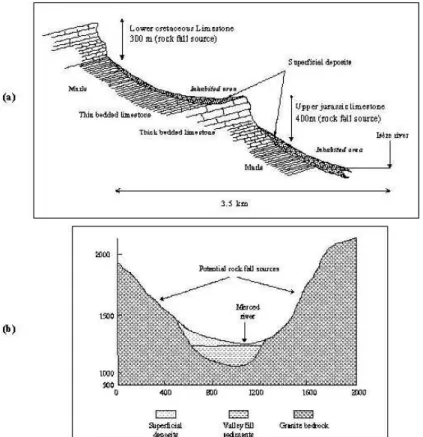
Fig. 1.Typical cross section of the cliffs concerned by the rock fall inventories.(a)Sub-vertical calcareous cliffs from the Chartreuse massif, Grenoble, France. Two main limestone levels are separated by a marly level.(b)Granitic cliffs from the Yosemite Valley, California, USA (scales in meter). The valley fill sediments consist of deltaic and lacustrine sediments, whereas the superficial deposits consist of rock fall and rock slide talus (after Wieczorek and J¨ager (1996), with permission).
to a few days) if the unstable slope is well instrumented and the movement follows specific processes (e.g. Azimi, 1996). In most cases no instrumentation is available. Long-term pre-dictions (a few years, a few decades or a few centuries) are only qualitatively estimated on the basis of the experience of an expert (e.g. Cancelli and Crosta, 1993; Hoek, 1998; Rouiller et al., 1998; Mazzoccola and Sciesa, 2000). The temporal evaluation appears to be the weakest point of rock fall hazard studies.
In other natural hazard fields, such as floods or earth-quakes, distribution laws have been proposed, based on sta-tistical analysis of historical data sets, to be representative for the observed frequency-size distribution of events. These laws, exponential-like for floods (e.g. Guillot and Duband, 1967; Water Resources Council, 1982) or power laws for earthquakes (Gutenberg and Richter, 1949), are widely used to derive a probabilistic recurrence rate of an event of a given size. More recently, this statistical approach has been ap-plied to landslides, with their surface distribution being well fitted by a power law (e.g. Hovius et al., 1997; Blodgett et al., 1996). This method allows for the calculation of erosion rates, as well as the probability of occurrence of a landslide of a given size. Some studies have shown that the volume distributions of rock falls from limited homogeneous areas are well fitted by a power law (Hungr et al., 1999 and
refer-ences therein; Dussauge et al., 2001). Due to the low number of available data sets, such studies are still rare.
We present the results of statistical analysis for 3 rock fall inventories, pointing out the possible biases when applied to hazard estimates. When comparing our observed volume dis-tributions to other ones proposed in the literature, common features appear, such as the shape of the law – a power law in all cases – and the exponent of this law. Then we discuss the opportunity to use this distribution law as a new tool for tem-poral hazard assessment. Several questions are raised about the validity of the law in both space and time domains. We point out the possibilities and limits of such an approach in the rock fall field, which still needs to be developed in order to answer the requirements of risk managers.
2 Statistical analysis of three rock fall inventories
2.1 Characteristics of rock fall inventories
Table 1.Characteristics of some rock fall volumes distributions
References Site Geological Number Time Sampled Range of the Exponent ba setting of events window volumes power law fit
(m3) (m3)
Gardner, 1970 Alberta, Canada, Calcareous 409 2 summer 10−6–10 10−2–10 0.72 natural cliffs and quartzitic rock periods
Our study, data Upper Arly gorges, Metamorphic and 59 22 years 5–104 20–3000 0.45±0.15 from Jeannin French Alps sedimentary rocks
(2001)
Our study, data Grenoble, French Calcareous 87 60 years 0.5–106 50–106 0.41±0.11
from RTM Alps cliffs
(1996)
Our study, data Yosemite Valley, Granitic cliffs 101 78 years 1–106 50–106 0.46±0.11 from Wieczoreck California
et al. (1992)
Dussauge et al. World wide Undifferentiated 142 10 000 103–2.1010 3.107–2.1010 0.52
(2001) rock cliffs years
British Columbia Massive felsic 389b,1 30 years 10−2–108 10−2–104 0.43 Hungr et al. Canada rock 123b,2 13 years 10−2–108 1–104 0.40 (1999) Road cuts Jointed 64b,3 – 10−2–108 1–104 0.70 metamorphic 122b,4 22 years 10−2–108 1–104 0.65
rock
Rousseau Mahaval, La Single natural 370 2 months Vmax= 1.5 order of 1 (1999) R´eunion, French basaltic cliff 9.106(c) magnitude
Island Instrumental measurements
aCumulative volume distribution and standard deviation.
bStudies on different locations in the same area: 1=Highway 99, bands A and B, 2=BCRailway, 3= Highway 1, 4=CP Railway. cDeduced from the amplitude of seismic signals (Rousseau, 1999).
Table 2. αvalues (n1) and annual number of rock falls larger than 100 m3, n100, calculated from the power-law distribution for 3 case studies. In order to compare values from spatially different areas, the coefficients are normalised by the surface of cliffs which are sources of events
Site α= n1 n100 Length of cliff Approximate n100/10 km2 (number/year) (number/year) considered (km) cliff surface (km2)
Grenoble area 4.2 0.62 120 24 0.26
Yosemite Valley 18∗ 2.16 100 30 0.72
Upper Arly gorges 8.5 1.07 2.2 0.55 –19.45–
extrapolated
∗In the Yosemite case, for an accurate calculation of thebvalue, the distribution law was studied only for a subset of the total data set –
onequarter with quantitative volume estimates (Dussauge et al., 2001). However, for theαcoefficient, the real number of events reported in the time window must be considered. The result of the sub-distribution (α= 4.5, Fig. 2) is multiplied by 4.
natural cliffs (Hungr et al., 1999). Second, hardly any in-strumental measurements exist for studying rock fall activ-ity. Luckman (1976) already pointed out this deficiency, and as far as we know no exhaustive field work has been pub-lished since this time. Most data are collected in the field by forest guards and rangers. Other ones are simply re-ported in historical archives. In particular, the volumes of each event are only roughly estimated, on the basis of the
scar in the cliff if possible, otherwise estimated in the de-position area. Recently, specific types of instrumentation, which initially aimed at monitoring other phenomena, such as volcanic eruptions, have been used to derive information about rock falls (Rousseau, 1999). This can be a future route to increase the number of instrumental data, but it has been seldom investigated up to now.
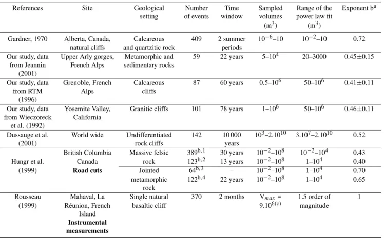
Fig. 2.Cumulative volume distributions for the rock fall records(a)Grenoble area, 87 records over 120 km of calcareous cliffs in the 1935– 1995 time window. The straight line represents the power law fit,f = 4.2V−0.41over the 50–106m3volume range. (b)Yosemite Valley, 101 records with quantitative volume estimates over 100 km of granite cliffs, 1915–1992. The power law is accepted over 50–106m3, with the equationf = 4.5V−0.46. The real number of data for this area over this time window – including data with qualitative volume estimates – is four times as high as what is used for the calculation ofb= 0.46. The valueα= 4.5 is thus four times as low as the real representative value.
fall data sets. In the time domain, the observation rate is not uniform. It depends on the visiting frequency of the different areas prospected, which is not always the same through the ages. For example, a rocky area may have been visited occa-sionally by forest guards during a century; if a road is built, the visits become daily. In the size domain, a clear under-estimation of small volumes in most inventories arises from two causes. First, when dealing with old past events, only the biggest ones, which have remained in human memory, are still to be found in the archives. Second, even nowa-days, rock falls are noticed mostly when they create
dam-age in forests, roads, and buildings. Hence, small events are seldom reported. This last remark also applies to a certain extent to inventories gathered along road cuts, the minimum volumes under which events are underestimated are lower than for natural cliffs.
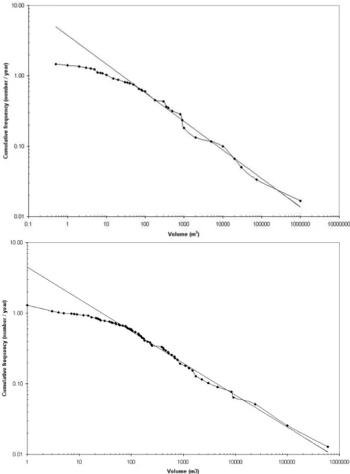
Fig. 3. Spatial distribution of the rock falls along the road 212 in the Arly gorges, Savoie, France, in the 1948–1996 period. Data from Jeannin (2001) with permission.
2.2 The Grenoble and Yosemite inventories: two regional-scale inventories
For the study of rock fall hazard assessment, we need to con-sider rock falls having their origin in natural cliffs, as well as on talus slopes or road cuts. We analysed two inventories with a similar time and space scale. Each one covers a large area with a series of natural rock cliffs varying in height. On each area, the geological setting can be considered as homo-geneous, i.e. the lithology and fracture pattern are roughly similar at the regional scale. However, the geological setting differs from one case to the other.
The first one concerns the calcareous cliffs of the Greno-ble area, French Alps. These cliffs are made of limestone and marls from the upper Jurassic and lower Cretaceous age. They represent altogether 120 km in length. They are 50 to 400 m high, with a mean value of 200 m. The morphology is mainly sub-vertical, the stratification dips gently inward (Fig. 1a). The discontinuity sets vary slightly from one loca-tion to another, but there are mainly three sub-vertical sets, one parallel to the direction of the cliff surface, and two oth-ers crossing it. The most common rock fall mechanisms are wedge failures, initiated on these two crossing sets, tower toppling and overhang failures, where the succession of lime-stone and marls suffer from differential erosion.
Forest guards from the RTM office have recorded rock falls since 1850 (RTM, 1996). Since the data collection is affected by the biases discussed previously, we only consider 88 events in the 1935–1995 time window (see also Dussauge et al., 2001). Rock fall volumes range from 0.5 to 106 m3.
The second inventory is representative of the Yosemite Valley, California, USA. It covers a cumulative length of 100 km of massive granite cliffs from the Cretaceous age,
which are up to 1000 m high, with a mean value of 300 m (Fig. 1b). These cliffs present mainly a round shape morphol-ogy, except for some steeper walls. They are characterised by an important set of discontinuities parallel to the topography. These discontinuities are responsible for a sheeting process, resulting from the release of pressure of previously buried rocks. Rock falls are partly induced by this sheeting pro-cess. The National Park rangers and USGS geologists have reported the occurrence of rock falls in the Yosemite Valley since 1850, gathering more than 400 events (Wieczorek et al., 1992). The distribution law was first tested on the whole set of data (Wieczorek et al., 1995). But among these data, only one-quarter has quantitative volume estimates. For a more accurate calculation of one parameter of the law (the
bvalue, see next section), with less biases, only 101 events with quantitative volume estimates have been taken into ac-count (Dussauge et al., 2001). They cover the 1915–1992 period (78 years) and the 1–6.105m3volume range.
For both inventories, rock fall volumes are primarily es-timated in the deposition area. These two data sets cover an area that is geologically homogeneous. They both went through several glaciations, the last one ending about 10 000 years ago (W¨urm in the Alps, Tioga in North America). They have been releasing from the weight of ice since this time and a few rock fall events have been triggered by earthquakes (around 10% in Yosemite and close to 0% in Grenoble area). The difference between the two series of cliffs is the lithol-ogy and the fracture systems, which induce different failure mechanisms for the rock falls.
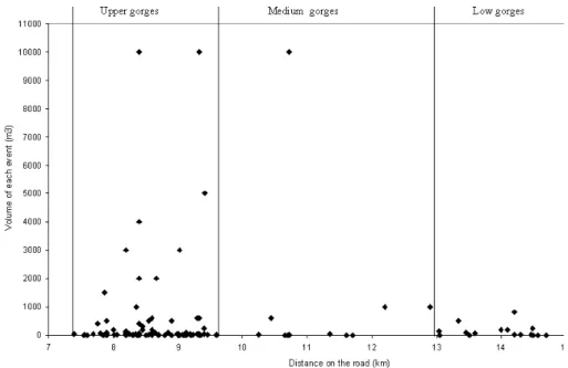
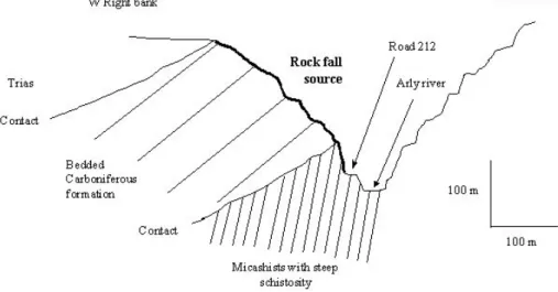
distribu-Fig. 4.Geological cross-section of the upper Arly gorges, Savoie, France. The rock fall source area is approximately 250 m high.
tion is statistically tested in order to find out the best fit over the wider range of volumes. Figure 2 presents the two distri-butions with a logarithmic scale. As described in Dussauge et al. (2001), the power-law distribution provides a good fit to the data, excluding exponential or Gumbel laws. Such a law is written
n(V )=αV−b, (1)
whereV is the volume,n(V )is the number of events per year with a volume greater thanV, andα andb are constants. Other laws with more parameters may provide a better fit, but we choose to use the minimum number of parameters, i.e. the simplest law for this first step analysis. Thebvalue can be estimated either from a linear regression method or by a maximum likelihood method. The maximum likelihood estimate forbis given by Aki, 1965.
b=1/Ln(10)(< logV >−logV0), (2) where< log(V ) >is the average value oflog(V ), andV0is the minimum volume considered, above which the catalogue is assumed to be complete. For the two data sets, the power law is accepted by aχ2 test for volumes larger than 50 m3 (χ2=5.2; see Dussauge et al., 2001). Under this value, the observed number of events per year is lower than the one expected from the power law. This lack of small volume compared to the theoretical law is probably due to the res-olution level of the sampling technique. Therefore, we study the rock fall volume distribution above this volumeV0. To determineV0, we test different threshold volumes, and we choose the minimum value ofV0 for which the power-law distribution is accepted by theχ2test and for which theb
value is constant, when we increase the threshold volume above V0. The linear regression and maximum likelihood methods provide similar values forbandα. The mean value appears in Table 1. We find similarbvalues for the two in-ventories, respectively, 0.41 for the Grenoble area and 0.46 for the Yosemite catalogue. The standard deviation of theb
value can be estimated using a maximum likelihood method and is given by (Aki, 1965)
σ =b/N−1/2, (3)
whereN is the number of events, andbis thebvalue from Eq. (1). Using Eq. (3), thebvalue standard deviation is equal to 0.11 for both Grenoble and Yosemite inventories. Thus, the difference between the two exponents is not statistically significant.
2.3 The Val d’Arly rock fall inventory: a local-scale inven-tory
In order to consider a smaller time and space scale, we study an inventory gathered in the Val d’Arly gorges, located be-tween Ugine and Flumet, Savoie, French Alps. This exam-ple allows for the analysis of a larger number of rock falls coming from a single cliff.
The road 212 was built on the flanks of these gorges at the beginning of the century. The local road service has noticed the extensive rock fall activity over a 7 km distance since 1954. It has reported daily every event larger than 1 m3, where debris has fallen on the road, causing momentary road closure. This procedure prevents the data from being affected by the bias discussed in Sect. 2.1, since the events are re-ported daily. An analysis of the spatial distribution of these rock falls shows a high concentration of events in the upper part of the gorges over 2.2 km (Fig. 3). On this section, 111 rock falls, from 1 to 10 000 m3, occurred from 1954 to 1994. Since protective structures, such as galleries and fences, have been built since 1976, thereby decreasing significantly the number of events, we only consider the time window from 1954–1976.
steeply dipping west. Above these mica schists are sedimen-tary rocks from the Carboniferous formation. They are com-posed of conglomerates and an alternation of sandstone and more crumbly shale. The stratification dips generally 40 to 50◦W, that is to say inward on the right bank. The main dis-continuity sets are the schistosity in the mica schists, which is very closely spaced, and the stratification in the Carbonif-erous formation. Three other sets of discontinuities affect both the mica schists and the Carboniferous formation and cut them into blocks (Jeannin, 2001).
Since most of the rock falls have their origin above the man-made cut, mainly in the Carboniferous formation, the influence of the road cut on the triggering of events is as-sumed to be weak. The main mechanism for rock falls is toppling, in the micaschists as well as in the Carboniferous formation.
In conclusion, the rock fall data gathered on the road sec-tion studied constitutes an inventory considered to be com-plete over 22 years. It includes 59 events occurring from a single natural cliff. The geological setting, identical over the whole area, is different from the previous cases, as well as the main rock fall mechanism.
The volume distribution of the rock falls is presented in Fig. 5. The data are well fitted by a power law in the range of 20–3000 m3. The exponent b, calculated with a linear regres-sion method, is equal to 0.45, with a standard deviation of 0.15. This value is very close to those found for the Greno-ble and Yosemite inventories. It is also in accordance with the values proposed by Hungr et al. (1999) for describing the volume distributions of rock falls from different road cuts in British Columbia, Canada.
An under-sampling of the data appears once more, under 20 m3. This value is not much lower than for the two previ-ous cases, – 50 m3. Some small volumes are stopped by the vegetation present on the slope, or they do not create much damage on the road and thus are not reported. However, if this value represents the resolution level associated with the sampling technique, it is surprising that the resolution level in this case is not much better than for the two previous cases – the minimum value for the validity of the law is not much lower than for inventories over broader areas. Also, the end of the distribution does not follow the theoretical power law, but this may be due to statistical fluctuations: the time win-dow is too short to be statistically representative of the rock fall activity for volumes greater than 3000 m3.
The power-law distribution is still statistically accepted by theχ2test, considering all volumes larger than 20 m3.
This example shows that a power law also represents the volume distribution of rock falls having their origin on a sin-gle cliff. Data from Gardner (1970), collected at the base of a single calcareous and quartzitic cliff in Alberta, Canada, during two summer periods, also show this power-law distri-bution for volumes ranging from 10−2to 10 m3. In this case, thebvalue is higher,b= 0.72. (Hungr et al., 1999).
3 Synthesis of the observed distribution patterns
Looking at different rock fall inventories (Table 1), the vol-ume distributions are fitted by a power law, at least above a given volume. In all cases, the distribution curve is flat for the smallest volumes and does not fit the power law. This is also observed for landslide size distributions. Stark and Hov-ius (2001) propose that this is a pure censoring effect, due to the sampling resolution, which does not challenge the over-all power-law behaviour. As well, power laws observed in the seismic field suffer a flat behaviour due to the monitoring resolution (Gutenberg and Richter, 1949). In addition, the re-sults for rock falls from our study and others, summarised in Table 1, show that this law is accepted regardless of the vol-ume range from 0.01–10 m3to 107–1010m3– or the period of observation – from two months to 10 000 years.
Such a distribution law could result from the variability of the cliff dimensions – height in particular – on the large areas considered (this aspect is further discussed in Dussauge et al., 2001). The inventories from the Arly gorges and the Alberta cliffs (Gardner, 1970), gathered on a single cliff, prove that the distribution law is not due to such a geometrical effect, i.e. an integration process over cliffs of different heights.
Rousseau (1999) reports rock falls from a single basaltic cliff on La R´eunion Island by recording the seismic signal produced by the failure. The volume of the events is cal-culated from the amplitude of the signal. The power law fits the volume distribution, withb= 1. This inventory, ob-tained from instrumental measurements, tends to show that the power-law behaviour is not a measurement artifact.
All these observations argue for the hypothesis that the power-law distribution well represents the rock fall volume distribution.
For all cases reported in Table 1, theb values show lit-tle variation. In particular, they are very close together for studies in the volume range 10–106m3, varying from 0.41 to 0.46 on natural cliffs. The comparison is interesting for the Grenoble and Yosemite inventories since they are based on the same scale of study – about 100 km of linear cliff for about 70 years. From a geologist’s point of view, it is a pri-ori surprising that the two areas present a similar rock fall distribution shape (power law with similarbvalue), because the fracturing patterns are fairly different for the two series of cliffs. However, the overall morphological patterns can be considered as similar, with high steep cliffs made of strong rock matrices. This suggests that the discontinuity patterns do not influence thebvalue of the volume distribution at this scale of study. At a lower scale – a few kilometers – Hungr et al. (1999) propose a higher value for more jointed rock (b= 0.65–0.70) than for massive rock (b= 0.40–0.43). The Arly study does not confirm this observation. Theb value of 0.45 characterizes closely jointed metamorphic and sedi-mentary rocks. Altogether, for the 10–106m3volume range,
bis roughly stable, i.e. close to 0.45.
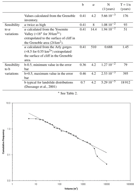
Table 3.Number per year n and return period T calculated for a rock fall with a volume larger than V=107m3, representative of the biggest historical rock falls reported in the Grenoble area in the last centuries. Sensibility to variations inαandbvalues
b α N T = 1/n
(1/years) (years)
Values calculated from the Grenoble 0.41 4.2 5.66 10−3 176 inventory.
Sensibility αtwice as high 0.41 8 1.08 10−2 93 toα αcalculated from the Yosemite 0.41 14.4 1.94 10−2 51 variations Valley (=18∗for 30 km2∗)
extrapolated to the surface of cliff in the Grenoble area (24 km2).
αcalculated from the Arly gorges 0.41 510 0.688 1.45 (=8.5 for 0.55 km2∗) extrapolated
the surface of cliff in the Grenoble area.
Sensibility b-0.5, minimum value in the error 0.36 4.2 1.27 10−2 79 to b bar
variations b+0.5, maximum value in the error 0.46 4.2 2.53 10−3 395 bar
b typical for landslide distributions 0.7 4.2 5.29 10−5 18 912 (Dussauge et al., 2001)
∗See Table 2.
Fig. 5. Cumulative frequency distribution for the rock fall volumes from the upper Arly gorges, France – 59 events recorded over 2.2 km between 1954 and 1976. The straight line represents the power-law fit, with the equationf= 8.5V−0.45over the 20–3000 m3volume range.
is characterized by ab value of 0.72, which is in the upper range of thebvalues reported for rock fall volumes (Gardner, 1970; Hungr et al., 1999). Assuming that this value is rep-resentative, two hypotheses are possible. On the one hand, it could be inferred that “small” and “big” phenomena do not behave in the same way. The “skin effect”, which affects the surface of rock slopes through temperature or thaw
At this stage of analyis, more data are required to carry out detailed statistical studies on various volume ranges.
The unique available data set built on instrumental mea-surements (Rousseau, 1999) provides us with a higher value, withb= 1. This may be due to the seismic model used for the derivation of the rock fall volumes, based on the amplitude of the seismic signal associated with the failure of a rock mass. This question is presently under investigation.
Theαcoefficient, as defined in Eq. (1), represents the an-nual number of events larger than 1 m3. Since such a small volume is not fitted by the power law, it makes no sense to discuss this value in a first step. On the contrary, all three power laws fit the data for a volumeV = 100 m3. We define
n100as the annual number of rock falls larger than 100 m3. With this definition,αis alson1. The values obtained from the three areas studied are reported in Table 2. In order to compare them on a homogeneous basis, eachn100coefficient is divided by the surface of cliffs that are potential sources of rock falls in the area . This surface is roughly estimated, us-ing the total length and approximate mean height.
Contrary to thebvalues, the normalizedn100coefficients fluctuate from one site to another, within at least two orders of magnitude. According to the distribution laws, a 10 km2 surface produces 0.26 events larger than 100 m3per year in the Grenoble area, 0.72 in the Yosemite Valley. The corre-sponding value extrapolated from the Arly gorges is 19.45.
4 Implications for rock fall hazard assessment
4.1 Principle of a statistical analysis of historical data Statistical analysis of past rock falls can provide a tool for quantifying future hazard in a probabilistic way. Dealing with a data set of events, the procedure to be followed can be divided into three steps.
1. The first step is to establish the volume distribution of the historical data. In order to work on a homogeneous temporal basis, we must select time windows where the rate of activity is almost constant. Statistical tests help to assess whether the distribution fits a mathematical law or not, at least over a certain range of volumes and a certain time window – for example, theχ2test (e.g. Press et al., 1992).
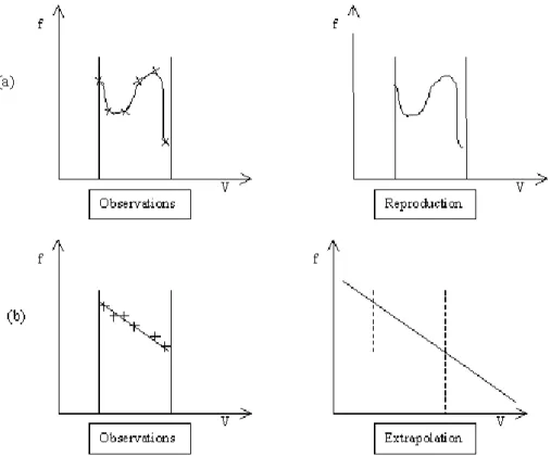
2. If the data do not fit any law, the inventory can be used to estimate an overall frequency for events with a vol-ume included in the volvol-ume range covered by the data (Fig. 6a). Assuming that the distribution is stationary in time, the observed distribution can be used for hazard assessment. No extrapolation is possible for volumes smaller or larger than those already observed.
3. If a law is accepted over a given range of volumes (for example, a power law), the parameters of the distribu-tion can be calculated using a graphic method or a max-imum likelihood method. The standard deviation of the
values can also be estimated using a maximum likeli-hood method, and this allows for an error bar to be es-timated for future previsions. In the case of a power law, theαcoefficient quantifies the level of activity of the area, i.e. the production of rock falls from whole cliffs in the area. However, if the power law does not fit the data down to 1 m3, as often observed, the correct coefficient to be taken into account isn(V0), the annual number of events larger thanV0, whereV0is the mini-mum volume fitted by the law.
A distribution law fitting the data is useful at least in two ways. First, within the volume range of historical observa-tion, the calculation of an annual number of events of a given volume (or larger than a given volume) provides a mean value which is less influenced by the statistical fluctuations inherent to observations on a short time window (Fig. 6b). Second, the law provides the possibility to extrapolate the observed distribution for smaller or larger volumes.
The number of events per yearn(V )can also be expressed as a return period T(V), with
T (V )=1/n(V ). (4) Note that a return periodT (V )= 25 years does not properly mean that an event larger than V occurs every 25 years, it is only an average over long periods – for example four events in a century.
4.2 Universal power-law distribution of rock fall volumes? Several authors have already proposed that the volume dis-tribution of rock falls is fitted by a power law (Hungr et al., 1999; Wieczorek et al., 1992; Dussauge et al., 2001). Our synthesis gives evidence that the exponent of this law may be site independent. This hypothesis is still difficult to assess with accuracy, since few data sets are available. However, if it can be proven true – through future studies of other in-ventories – it would provide an interesting tool for assessing rock fall hazards, when coupled with a discussion about the
αcoefficient.
Indeed, a power law with a constantbvalue would work as an equivalent for the earthquake size distribution (e.g. Guten-berg and Richter, 1949). The observed earthquake sizes fit the law
N (M)=αM−b, (5)
where M is the seismic moment (measuring the energy of an earthquake) andN (M)is the number of earthquakes of a seismic moment larger thanM. Among others, Main (1996) argues for the stationarity of this law, that is to say the statis-tical properties of the earthquake frequency-size distribution remain constant in time. In addition, since the earthquake in-ventories are instrumental, they are considered complete, at least above a given size (resolution level). The parameterα
Fig. 6.Schematic representation of possible uses of historical data sets.(a)When the data do not fit any distribution law, the only possibility is to reproduce the distribution over the same volume range. (b)When a power law (or another kind of law) is accepted, the estimation of rock fall frequencies is improved and the distribution can be extrapolated outside the volume range (and time window).
used to derive the future occurrence rate of earthquakes of a given magnitude from past short-term instrumental invento-ries (e.g. Reiter, 1991).
Drawing a tight parallel to this approach, the power-law distribution of rock fall volumes discussed in Sect. 3 raises important questions. First, is the distribution law stationary over time? Available inventories are not long enough to anal-yse the temporal variability of the rock fall volume distribu-tion. Wasowski and Del Gaudio (2000) suggested that prob-abilistic temporal hazard estimates of slope failures can be possible provided that the interval for data completeness is much longer than the event recurrence period. However, the rock fall activity may depend on the loading conditions, in-cluding climate or triggering by earthquakes. This may lead to temporal fluctuations of the rock fall activity, and possibly of thebvalue. Lateltin et al. (1997) point out a relationship between climate change and landslide activity in Switzerland for rather shallow phenomena, whereas deeper phenomena seem to be little influenced (Noverraz et al., 1998). A posi-tive answer to the question about stationarity would validate the calculation of a recurrence rate of future events of a given size on the basis of the occurrence of past events.
Second, is theb value site independent? In the examples studied, the distribution law does not seem to depend on the site considered. For the same range of volumes, thebvalues are similar regardless of the geological settings – limestone and marls in the Grenoble area, granite in the Yosemite
Val-ley, metamorphic rocks in the Arly gorges, felsic rocks in British Columbia (Table 1). On the other hand, theb val-ues reported in various regions for the distribution of land-slides in soil materials only are generally higher than 0.6–0.8 (when recalculated on the basis of homogeneous criteria, i.e. cumulative distribution of volumes of moving material, as described in Dussauge et al., 2001 and references therein). One hypothesis to explain these observations is that the con-trol parameter for the slope movements is the overall strength of the material. This is in accordance with the erosion model proposed by Densmore et al. (1998). The b value of the distribution law of the slope movements involved in erosion processes increases when the geomechanical properties of the slope –c, φ – decrease. More rock fall and landslide data sets, in regions with various homogeneous geomechan-ical features, will help to enforce this hypothesis.
Third, how can we compare the rock fall activity for dif-ferent sites or for difdif-ferent spatial scales? As an example, the spatial distribution of the rock falls in the Arly gorges is not uniform (Fig. 3). The rock fall activity is primarily concen-trated in a narrow corridor. Therefore, the rock fall activity, measured as theαcoefficient in Eq. (1), for the most active area, cannot be extrapolated for all of the Arly gorges. This extrapolation would induce an overestimation of the rock fall hazard.
the Arly gorges is far higher than those for the Grenoble area and Yosemite Valley. If we extrapolate the activity for the upper Arly gorges – rock falls concentrated on 0.55 km2– to the surface of the Grenoble area – approximately 24 km2, we should observe 47 rock falls per year of volume larger than 100 m3 instead of the 0.6 events per year recorded for the Grenoble catalogue (Table 2).
In conclusion, trends are already emerging for the exis-tence of a power law representing the rock fall volume distri-butions. Thebvalue seems to be site independent for areas with similar rock material properties –b= 0.46±0.06, ex-cept for the studies from Rousseau (1999) and Hungr et al. (1999) (Table 1) – whereas theαcoefficient is spatially vari-able over several orders of magnitude. The important ques-tion is how to isolate homogeneous areas regardingαandb. We suggest investigating a possible correlation between the
αandbparameters and the geological, geomechanical mor-phological and climatic settings. It would then become con-ceivable to estimate rock fall frequencies where no inventory is available.
4.3 Extrapolation possibilities
At the present stage, for a given site, we can extract from historical data sets some information on rock fall patterns in the size, space, and time domains implied in the observation. One century of complete observations can be used to pro-pose the expected values for the next century, for the same area and the same range of rock fall volumes. In addition, in terms of hazard analysis, the 102to 106m3range of vol-umes is of particular interest to risk managers dealing with land use at medium or long-time scales, i.e. a few years to a few decades – small block falls cause many accidents but are dealt with at a short time scale, i.e. a few months (e.g. Interreg IIc, 2001). This range is actually the one best fitted by a power law and probably the most completely reported. For example, in the Grenoble area, the distribution allows us to expect a decennial event of 104m3, or an average of four 105m3events within a century.
The extrapolation of this law to small volumes is still deli-cate due to sampling resolution, as already discussed. On the other extreme, the extrapolation to larger volumes must be handled carefully. As shown in Table 3, it is very sensitive to theαandbvalues chosen for the power law. Such extrapola-tions are only feasible when the limits of the inventory used are very well defined, i.e. statistical tests certify its complete-ness, andαandbare well constrained. However, even if the error bars are large, extrapolated recurrence rates can be es-timated. It would not be possible without the existence of a distribution law. For our study, a first indicator for the ro-bustness of the law is given by the existence of a power law with similarbvalues for data collected over different volume ranges, space scales and period lengths: 0.01–10 m3, a few hundreds of m2and 2 summer periods in Alberta (Gardner, 1970; Hungr et al., 1999), 50–106 m3, 30 km2and 80 years in Yosemite (Wieczorek et al., 1992; Dussauge et al., 2001).
These observations validate the extrapolation of the rock fall volume distribution to volumes larger than the available data. 4.4 Hazard assessment
As requested by risk managers, evaluating rock fall hazard includes estimating the probability of failure of identified rock masses within a given period of time. Our study shows that statistical studies of past events provide a tool for quanti-fying an overall frequency of rock falls on a given area (at the scale of a whole cliff or series of cliffs). This is not yet the probability of occurrence of a specific instability. As a paral-lel, data sets of historical seismicity help to estimate the prob-ability of occurrence of an earthquake of a given magnitude, but not predicting exactly where it will occur (frequency of events). The statistical spatial distribution of the events asso-ciated with a propagation law (attenuation of the horizontal ground acceleration with the distance) is the basis for build-ing probabilistic seismic hazard maps (e.g. Dominique et al., 1998; Romeo et Pugliese, 1998). On the other hand, pointing out the locations most susceptible for a rock failure is local field work (at the scale of specific rock masses), based on geological and geomechanical considerations, which leads to characterization of potential instabilities. The crossing of these two approaches aims at estimating the individual prob-ability of failure for a specific instprob-ability, which is the final goal of such a process (Vengeon et al., 2001).
5 Conclusion
The observation of several rock fall inventories shows that a power-law distribution (Eq. (1)) fits the data for a given range of volumes. For various types of rock cliffs, thebvalues are similar – 0.41 to 0.46 – whereas theαvalues (more precesely
n100/10 km2) vary within at least two orders of magnitude. The existence of such a law provides interesting opportuni-ties for a probabilistic assessment of rock fall hazards. First, the application of the distribution law improves the estima-tion of a mean recurrence rate for events in the volume range of the reported data. The fluctuation of the values observed in short-time windows are smoothed. Second, it gives the possibility to extrapolate the distribution for large events that are not reported in the observed period.
Acknowledgements. We gratefully thank P. Desvarreux and the S.A.G.E engineering office, J.P. Requillard and the R.T.M. office, and G. Wieczorek, who made the data available for the three in-ventories we used in this study, respectively Arly gorges, Greno-ble area and Yosemite Valley. Comments by G. Wieczorek and re-view by G.B. Crosta and J. Wasowski improved the quality of the manuscript. J.M. Vengeon is acknowledged for his useful discus-sions.
References
Aki, K.: Maximum likelihood estimation of b in the formula
log(N )= a−bM and its confidence limits, Bull. Earthquake Res. Inst., Tokyo Univ., 43, 237–239, 1965.
Azimi, C. and Desvarreux, P.: Quelques aspects de la pr´evision des mouvements des terrain, Revue franc¸aise de g´eotechnique, 76, 63–75, 1996.
Blodgett, T. A., Isacks, B. L., Fielding, E. J., Masek, J. G., and Warner, A. S.: Erosion attibuted to landslides in the Cordillera Real, Bolivia, Eos Trans. AGU, 17, 17, Spring Meet. Suppl. S261, 1996.
Cancelli, A. and Crosta, G.: Rockfall hazard in Italy: assessment, mitigation and control, in Environment management, geo-water and engineering aspects, Balkema, Wollongong, 1993.
Densmore, A., Ellis, M., and Anderson, R.: Landsliding and the evolution of normal-fault-bounded mountains, J. Geophys. Res., 103, 7, 203–219, 1998.
Dominique, P., Autran, A., Bl`es, J. L., Samarcq, F., and Terrier, M.: Probabilistic approach: seismic hazard map on the national territory (France), in 11th Eur. Conf. on Earthquake Engineering, Balkema, Paris, 1998.
Dussauge, C., Grasso, J. R., and Helmstetter, A.: Statistical analysis of rock falls: implication for hazard assessment and underlying physical processes, J. Geophys. Res, submitted, 2001.
Erisman, T. H. and Abele, G.: Dynamics of rockslides and rockfalls, Springer, 2001.
Gardner, J.: Rockfall: a geomorphic process in high mountain ter-rain, The Albertan Geographer, 6, 15–20, 1970.
Guillot, P. and Duband, R.: La m´ethode du GRADEX pour le calcul de probabilit´e de crues `a partir des pluies, IASH Publication (84), 1967.
Gutenberg, B. and Richter, F.: Seismicity of the earth and associated phenomena, Princeton Univ. Press, Princeton, N. J., 1949. Hoek, E.: Analysis of rock fall hazards, in Rock Engineering,
Course notes; Chapter 9; http://www.rockeng.utoronto.ca/ hoek-corner.htm, 115–136, 1998.
Hovius, N., Stark, C. P., and Allen, P. A.: Sediment flux from a mountain belt derived by landslide mapping, Geology, 25, 3, 231–234, 1997.
Hungr, O., Evans, S. G., and Hazzard, J.: Magnitude and frequency of rock falls along the main transportation corridors of south-western British Columbia, Canadian Geotechnical Journal, 36, 224–238, 1999.
Interreg IIc: Pr´evention des mouvements de versants et des insta-bilit´es de falaise – Groupe falaise – Confrontation des m´ethodes d’´etude des ´eboulements rocheux dans l’arc alpin, Programme Interreg IIc, Mditerran´ee occidentale et Alpes Latines, 2001. Jeannin, M.: Approches quantitatives de l’´erosion des versants
rocheux. Etude des gorges de l’Arly et du sillon subalpin. DEA report, Lirigm, Univ. Joseph Fourier, Grenoble, 2001.
Lateltin, O., Beer, C., Raetzo, H., and Caron, C.: Instabilit´es de pente en terrain de flysch et changements climatiques. Rapport final PNR 31, 168, Z¨urich, 1997.
Luckman, B. H.: Rockfalls and rock fall inventory data: some ob-servations from Surprise Valley, Jasper National Park, Canada, Earth Surface Processes, 1, 287–298, 1976.
Main, I.: Statistical Physics, seismogenesis and seismic hazard, Re-views of Geophysics, 34, 4, 433–462, 1996.
Mazzoccola, D. and Sciesa, E.: Implementation and comparison of different methods for rock fall hazard assessment in the Italian Alps, in 8th Int. Symp. on Landslides, 1035–1040, Cardiff, UK, 2000.
Noverraz, F., Bonnard, C., Dupraz, H., and Huguenin, L.: Grands glissements de versants et climat, VERSINCLIM: Comporte-ment pass´e, pr´esent et futur des grands versants instables sub-actifs en fonction de l’´evolution climatique, et ´evolution en con-tinu des mouvements en profondeur. Rapport final PNR 31, 314, Z¨urich, 1998.
Press, W. H., Teukolsky, S. A., Vettering, W. T., and Flannery, B. P.: Numerical recipes in C, Cambridge Univ. Press, 994, Cambridge, 1992.
Reiter, L.: Earthquake hazard analysis, Columbia Univ. Press, New York, 1991.
Romeo, R. and Pugliese, A.: A global earthquake hazard assess-ment of Italy, in 11th Eur. Conf. on Earthquake Engineering, Balkema, Paris, 1998.
Rouiller, J. D., Jaboyedoff, M., Marro, C., Philippossian, F., and Mamin, M.: Pentes instables dans le Pennique valaisan, MAT-TEROCK: une m´ethodologie d’auscultation des falaises et de d´etection des ´eboulements majeurs potentiels, Rapport final PNR 31, edited by vdf Hochschulverlag AG an der ETH, 239, Z¨urich, 1998.
Rousseau, N.: Study of seismic signals associated with rockfalls at 2 sites on the Reunion island (Mahavel Cascade and Souffri`ere cavity), PhD Thesis, IPG, Paris, 1999.
RTM Is`ere: Inventaire des mouvements rocheux, Secteur de l’Y grenoblois, Service de Restauration des terrains en Montagne de l’Is`ere, Grenoble, France, 1996.
Stark, C. P. and Hovius, N.: The characterisation of landslides size distributions, Geophys. Res. lett., 26, 6, 1091–1094, 2001. Vengeon, J. M., Hantz, D., and Dussauge, C.: Predictabilit´e
des ´eboulements rocheux: approche probabiliste par combinai-son d’´etudes historiques et g´eom´ecaniques, Revue Francaise Geotechnique, 95–96, 1, 2001.
Wasowski, J. and Del Gaudio, V.: Evaluating seismically induced mass movement hazard in Caranico Terme (Italy), Eng. Geol., 58, 291–311, 2000.
Water Resources Council: Guidelines for determining flood flow frequency, Bulletin 17B: Hydrology subcommitee, Office of Wa-ter Data Coordination, US Geological Survey, Reston, VA, 182, 1982.
Wieczorek, G. and J¨ager, S.: Triggering mechanisms and depo-sitional rates of postglacial slope movement processes in the Yosemite Valley, California, Geomorphology, 15, 17–31, 1996. Wieczorek, G., Nishenko, S. P., and Varnes, D. J.: Analysis of rock
falls in the Yosemite Valley, California, in 35th US Symposium on Rock Mechanics, edited by J. J. Daemen, and Schultz, R. A, 85–89, A. A. Balkema, Daemen, 1995.