Fundação Getúlio Vargas
Escola Brasileira de Economia e Finanças
Cristina Tessari
Dois Ensaios em Finanças
Cristina Tessari
Dois Ensaios em Finanças
Dissertação submetida à Escola
Brasileira de Economia e Finanças
como requisito parcial para a
obtenção do grau de Mestre em
Economia
Área de concentração: Finanças
Orientador: Caio Ibsen Rodrigues
de Almeida
Ficha catalográfica elaborada pela Biblioteca Mario Henrique Simonsen/FGV
Tessari, Cristina
Dois ensaios em finanças / Cristina Tessari. – 2016. 81 f.
Dissertação (mestrado) - Fundação Getulio Vargas, Escola de Pós- Graduação em Economia.
Orientador: Caio Ibsen Rodrigues de Almeida. Inclui bibliografia.
Agradecimentos
Agradeço,
Ao meu orientador Caio Almeida, pela fundamental contribuição para o desenvolvi-mento e conclusão deste trabalho, pelas ideias, sempre brilhantes, pela compreensão, força, amizade, e carinho. Sou grata pela extrema gentileza, disponibilidade e grandiosas sugestões e ideias para os artigos, pela paciência, e por me mostrar que o único caminho possível era o da dedicação.
Aos membros da Banca Examinadora, pelo tempo dispensado na leitura deste trabalho e pelos comentários e críticas.
Ao meu co-autor Bernardo Ricca, pela grande dedicação, objetivas e cruciais con-tribuições no segundo capítulo desta dissertação.
A todo o corpo docente da EPGE, por me ensinar uma nova maneira de pensar, pelo compromisso com a excelência acadêmica e pela vital contribuição para a minha formação.
Aos funcionários da EPGE, por todo o apoio.
A todos os meus colegas da EPGE, pelas conversas e debates no hall dos elevadores,
pelas muitas dúvidas tiradas, pela amizade e companheirismo durante esses anos de con-vivência.
Aos meus pais Celso e Aidi, por estarem sempre por perto, pelo apoio, carinho e compreensão ao longo de toda a minha vida, por sempre terem acreditado na minha capacidade, enquanto muitos outros duvidaram, por terem me dado plena liberdade para fazer as minhas escolhas, mesmo sem entender muitas delas, e por nunca terem interferido nas minhas decisões.
Sumário
1 Option Pricing under Multiscale Stochastic Volatility 10
1.1 Introduction . . . 11
1.2 A Model for the Stock Price Dynamics . . . 13
1.2.1 The Model . . . 13
1.2.2 Pricing Equation . . . 15
1.2.3 The Variogram and Time Scales in Market Data . . . 17
1.2.4 Implied Volatility Asymptotic and Calibration . . . 19
1.3 Numerical Results. . . 21
1.3.1 Data Description . . . 21
1.3.2 Mean-Reversion Rates and Block Bootstrap . . . 22
1.3.3 Calibration Results . . . 24
1.3.4 Numeric Examples . . . 31
1.3.5 Application: Pricing an Exotic Derivative . . . 35
1.4 Concluding Remarks . . . 35
Appendix . . . 36
1.A Properties of the Variogram Estimator . . . 36
1.B First-Order Perturbation Theory . . . 39
2 Idiosyncratic Moments and the Cross-Section of Stock Returns in Brazil 46 2.1 Introduction . . . 47
2.2 Data and Variables . . . 50
2.2.1 Data Description . . . 50
2.2.2 Construction of Variables . . . 51
2.3 Constructing Moment-Based Portfolios . . . 61
2.3.1 Sorting Stock Returns on Expected Idiosyncratic Skewness . . . 61
2.3.2 Sorting Stock Returns on Realized Idiosyncratic Skewness . . . 63
2.3.3 Sorting Stock Returns on Realized Idiosyncratic Volatility . . . 65
2.4 Robustness Analysis . . . 68
2.4.1 Tercile Portfolios . . . 68
2.4.3 Return Reversal . . . 73
2.5 Concluding Remarks . . . 75
Lista de Figuras
1.1 The empirical variogram for the S&P 500 volatility process . . . 23
1.2 Bootstrap distributions of the sample parameters . . . 25
1.3 Data and calibrated fit on November 03, 2015. . . 27
1.4 Data and calibrated fit on November 03, 2015 (slow scale). . . 28
1.5 Implied volatility fit of S&P 500 index options on November 03, 2015. . . 29
2.1 Cumulative returns of the three Fama-French factors . . . 52
2.2 Cross-sectional distribution of firm-level volatility . . . 55
Lista de Tabelas
1.1 Summary statistics of the estimates of the model variogram (1.26). . . 24
1.2 Estimated values of the group market parameters . . . 30
1.3 Root mean square error (RMSE) . . . 31
1.4 Ratio between the correction termP1 and the total price P∗ . . . 31
1.5 Parameters and initial conditions used in the two-factor stochastic volatility model (1.3). . . 32
1.6 Root mean square error (RMSE) . . . 33
1.7 Ratio between the correction termP1 and the total price P∗ . . . 34
2.1 Descriptive statistics of the three Fama-French factors . . . 51
2.2 Significance of the three Fama-French factors across regressions . . . 54
2.3 Descriptive statistics of skewness predictor variables . . . 58
2.4 Skewness predictive regressions . . . 60
2.5 Root mean squared error (RMSE) . . . 61
2.6 Summary statistics for portfolios formed on expected idiosyncratic skewness 64 2.7 Summary statistics for portfolios formed on realized idiosyncratic skewness 66 2.8 Summary statistics for portfolios formed on realized idiosyncratic volatility 67 2.9 Summary statistics for portfolios formed on expected idiosyncratic skewness 70 2.10 Summary statistics for portfolios formed on realized idiosyncratic skewness 71 2.11 Summary statistics for portfolios formed on realized idiosyncratic volatility 72 2.12 Summary statistics for equally-weighted portfolios sorted on idiosyncratic moments . . . 74
Capítulo 1
Option Pricing under Multiscale
Stochastic Volatility
Abstract
In this paper, we test some stochastic volatility models using options on the S&P 500 index. First, we demonstrate the presence of a short time-scale, on the order of days, and a long time-scale, on the order of months, in the S&P 500 volatility process using the empirical structure function, or vari-ogram. This result is consistent with findings of previous studies. The main contribution of our paper is to estimate the two time-scales in the volatility process simultaneously by using nonlinear weighted least-squares technique. To test the statistical significance of the rates of mean-reversion, we bootstrap
pairs of residuals using the circular block bootstrap of Politis and Romano
(1992). We choose the block-length according to the automatic procedure of
Politis and White (2004). After that, we calculate a first-order correction to the Black-Scholes prices using three different first-order corrections: (i) a fast time scale correction; (ii) a slow time scale correction; and (iii) a multiscale (fast and slow) correction. To test the ability of our model to price options, we simulate options prices using five different specifications for the rates or mean-reversion. We did not find any evidence that these asymptotic models perform better, in terms of RMSE, than the Black-Scholes model.
1.1
Introduction
Asset return volatility is a central concept in finance, whether in asset pricing, portfolio selection, or risk management. Although many well-known theoretical models assumed
constant volatility (seeMerton,1969;Black and Scholes,1973), sinceEngle(1982) seminal
paper on ARCH models, the financial literature has widely acknowledge that volatility is
time-varying, in a persistent fashion, and predictable (seeAndersen and Bollerslev,1997).
From the point of view of derivative pricing and hedging, continuous time stochastic volatility models, which can be seen as continuous time versions of ARCH-type models, have become popular in the last twenty years. The idea of using stochastic volatility models to describe the dynamics of an asset price comes from empirical evidence indicating that asset price dynamics is driven by processes with time-varying volatility. In fact, two
phenomena are observed: (i) a non-flat implied volatility surface when the Black and
Scholes (1973) model is used to interpret financial data, and (ii) skewness and kurtosis are present in the asset price probability density function deduced from empirical data. These phenomena stands in empirical contradiction to the consistent use of a classical Black-Scholes approach to price options and similar securities, as the Black–Scholes model fails to correctly describe the market behavior.
Stochastic volatility models relax the constant volatility assumption of the Black-Scholes model by allowing volatility to follow a random process. In this context, the market is incomplete because the volatility is not traded and the volatility risk cannot be fully hedged using the basic instruments (stocks and bonds). To preclude arbitrage, the market selects a unique risk neutral derivative pricing measure, from a family of possible measures. As a result, in contrast to the Black-Scholes model, the stochastic volatil-ity models are able to capture some of the well-known features of the implied volatilvolatil-ity surface, such as the volatility smile and skew.
The presence of volatility factors is well documented in the literature using underlying
returns data (seeAlizadeh et al.,2002;Andersen and Bollerslev,1997;Chernov et al.,2003;
Engle and Patton,2001;Fouque et al.,2003b;Hillebrand,2005;LeBaron,2001;Gatheral,
2006, for instance). While some single-factor diffusion stochastic volatility models such as
Heston(1993) enjoy wide success, numerous empirical studies of real data have shown that the two-factor stochastic volatility models can produce the observed kurtosis, fat-tailed
return distributions and long memory effect. For example,Alizadeh, Brandt, and Diebold
(2002) used ranged-based estimation to indicate the existence of two volatility factors
including one highly persistent factor and one quickly mean-reverting factor. Chernov,
that two factors are necessary for log-linear models. Those evidences, among others, have motivated the development of multiscale stochastic volatility models as an efficient way to capture the principle effects on derivative pricing and portfolio optimization of randomly varying volatility.
In this paper, motivated by both the popularity and appeal of stochastic volatility models and by the difficulty associated with their estimation, we compare the performance
of three different specifications of theFouque, Papanicolaou, and Sircar(2000)’s stochastic
volatility model for pricing European call options. We assume that the underlying asset
evolves according to a geometric Brownian motion, as in the Black and Scholes (1973)
model, but with stochastic volatility. We use S&P 500 data to demonstrate that the volatility of this index is driven by two diffusions: one fast mean-reverting and one slow-varying. In order to identify these scales, we analyze low- and high-frequency data using the empirical structure function, or variogram, of the log absolute returns. To retrieve the scale on the order of months, we use daily closing prices of the S&P 500 over several
years. To extract the scale on the order of days, we follow Fouque et al. (2003a) and use
high-frequency, intraday data.
In their work, Fouque, Papanicolaou, and Sircar (2000) show that multiscale
stochas-tic volatility models lead to a first-order approximation of the implied volatility surface and derivative prices. By using a combination of singular and regular perturbations to approximate prices when the volatility is driven by short and long time-scale factors, they derive a first-order approximation for European options prices and their induced implied volatilities. This first-order approximation is composed by the Black-Scholes price and the first-order correction involves only Greeks. In terms of implied volatility, this pertur-bation analysis translates into an affine approximation in the log-moneyness to maturity ratio (LMMR). This perturbation method allows a direct calibration using real data of the group market parameters, which are exactly those needed to price exotic contracts at this level of approximation. The advantage of this approach is that the resulting formula for the option price does not depend on the unobserved current value of the volatil-ity. However, calibration of this model requires information on near-the-money implied volatilities.
We have three different goals in this work. First, to demonstrate the presence of a well-identified short time-scale (on the order of a few days) and a long time-scale (on the order of months) in the S&P 500 volatility process. In order to do that, we show that the fast time-scale and the slow time-scale can be simultaneously estimated by using two different datasets, making use of the empirical structure function, or variogram. To test the statistical significance of the speeds of mean-reversion, we use the circular block
block-length selection of Politis and White (2004). The second goal, conditional on the market supporting evidence of a multiscale stochastic volatility process, is related to the calibration of the model using option data on the underlying. At this stage, we compare the observed prices with the corrected Black-Scholes prices by using three different first-order corrections: (i) a fast time scale correction; (ii) a slow time scale correction; and (iii) a multiscale correction (fast and slow). Finally, the third goal of this paper is to simulate trajectories of corrected prices and price an exotic derivative (digital option).
The rest of this paper proceeds as follows. In Section 2, we describe the class of multiscale stochastic volatility models that we will work with. In Section 2.3, we present the empirical structure function, or variogram, which is used as an estimator of the speed of mean reversion. In Section 2.4, we present the first-order approximation derived in
Fouque, Papanicolaou, and Sircar (2000), which is valid for any European-style option. Additionally, we present an explicit formula for the implied volatility surface induced by the option pricing approximation. In Section 3, we report the numerical results. In Section 4, we show how the corrected Black-Scholes prices can be used to price exotic options. Finally, Section 5 concludes.
1.2
A Model for the Stock Price Dynamics
1.2.1
The Model
Let (Ω,F,P,{Ft}t≥0) be a complete probability space with a filtration satisfying the
usual conditions. We consider a family of stochastic volatility models (Xt, Yt, Zt), where
Xt is the underlying price, and Yt and Zt are two mean-reverting Ornstein–Uhlenbeck
(OU) processes. Under the physical probability measure P, our model can be written as
the following system of stochastic differential equations (SDE):
dXt =µXtdt+f(Yt, Zt)XtdWt0, dYt = 1ǫα(Yt)dt+ √1ǫβ(Yt)dWt1, dZt =δc(Zt)dt+
√
δg(Zt)dWt2,
(1.1)
where (W(0), W(1), W(2)) are correlated
P-Brownian motions with
dWt(0)dWt(i) =ρidt, i= 1,2, dWt(1)dW
(2)
t =ρ12dt, (1.2)
and |ρ1| < 1, |ρ2| < 1, |ρ12| < 1, and 1 + 2ρ1ρ2ρ12 −ρ21 −ρ22 − ρ212 > 0 in order to
underlying price Xt evolves as a diffusion with geometric growth rate µ and stochastic
volatilityσt =f(Yt, Zt).1 The fast volatility factorYt evolves with a mean reversion time
ǫ, while the slow volatility factor Zt evolves with a time scale 1/δ. In order to have a
separation of scales, we must assume thatδ ≪1/ǫ.
Here, it is worth mentioning that this model characterizes an incomplete market, in
contrast to the Black and Scholes (1973) model, since the volatility presents its own
in-dependent sources of uncertainty, Yt and Zt. The introduction of these two new sources
of randomness give rise to a family of equivalent martingale measures that will be
pa-rameterized by the market price of risk,λ(y, z) = (µ−r)/f(y, z), and two market prices
of volatility risk, which we denote by ξ(y, z) and ζ(y, z), associated with Yt and Zt,
re-spectively. All these market prices are not determined within the model, but are fixed exogenously by the market. To preclude arbitrage, we assume that the market chooses
one measureP∗ through the combined market price of volatility risk (ξ, ζ).
Under the risk neutral measure P∗, an application of the Girsanov theorem provides
that our model can be written as
dXt =rXtdt+f(Yt, Zt)XtdWt0∗, dYt =
1
ǫα(Yt)−
1
√
ǫβ(Yt)Λ1(Yt, Zt)
dt+ √1
ǫβ(Yt)dW
1∗
t , dZt =
δc(Zt)− √
δg(Zt)Λ2(Yt, Zt)
dt+√δg(Zt)dWt2∗,
(1.3)
wheref is a positive function, bounded above and away from zero, r ≥0 is the risk-free
rate of interest, and the combined market prices of volatility risk associated with Yt and
Zt are
Λ1(y, z) =ρ1λ(y, z) +ξ(y, z)
q
1−ρ2
1, (1.4)
Λ2(y, z) =ρ2λ(y, z) +ξ(y, z)ρ12+ζ(y, z)
q
1−ρ2
2−ρ212. (1.5)
In our model, the coefficientsα(y) =mY −y and β(y) =νY√2 describe the dynamics
of Y under the physical measure P and the coefficients c(z) =mZ−z and g(z) =νZ√2
describe the dynamics of Z under P. Their particular form does not play a role in
the perturbation analysis provided that they are defined so that the processes Y and
Z are mean-reverting and have a unique invariant distribution denoted by ΦY and ΦZ,
respectively. SinceY andZare OU processes, it can be shown that ΦY is the density of the
normal distributionN(mY, νY2), where νY2 =β2/2α, and ΦZ is the density of the normal
1
If σt is constant, then Xt is a geometric Brownian motion and corresponds to the classical model
distribution N(mZ, νZ).2 Finally, the P∗-standard Brownian motions (Wt0∗, Wt1∗, Wt2∗)
present the same correlation structure as between theirP-counterparts in Equation (1.2).
1.2.2
Pricing Equation
Consider a European option with smooth and bounded payoff functionh(x) and
expira-tion dateT. The fact that the discounted price ˜Pt=e−rtPtis aP∗-martingale guarantees
that the no-arbitrage pricing function of this option at timet < T is given by
Pǫ,δ(t, Xt, Yt, Zt) =E∗ n
e−r(T−t)h(XT)
Xt, Yt, Zt o
, (1.6)
where the expectation E∗{·} is taken under the risk-neutral pricing measure P∗, and the
Markov property of (Xt, Yt, Zt) is used. By an application of the Feynman-Kac formula,
we obtain a characterization of Pǫ,δ as the solution of the parabolic partial differential
equation (PDE)
∂Pǫ,δ
∂t +L(X,Y,Z)P
ǫ,δ −rPǫ,δ = 0, (1.7)
with terminal conditionPǫ,δ(T, x, y, z) =h(x), whereL
(X,Y,Z)is the infinitesimal generator
of the Markov processes (Xt, Yt, Zt). Define the infinitesimal generator Lǫ,δ as
Lǫ,δ = ∂t∂ +L(X,Y,Z)−r, (1.8)
so that (1.7) can be written as
Lǫ,δPǫ,δ = 0, (1.9)
with terminal condition Pǫ,δ(T, x, y, z) = h(x). It is convenient to re-write the operator
Lǫ,δ as a sum of components that are scaled by the different powers of the small parameters
(ǫ, δ) that appear in the infinitesimal generator of (X, Y, Z) as
Lǫ,δ = 1ǫL0+ 1
√
ǫL1+L2+ √
δM1+δM2+
s
δ
ǫM3, (1.10)
where the operators are defined as
L0 = 1
2β
2(y) ∂2
∂y2 +α(y)
∂
∂y, (1.11)
L1 =β(y) ρ1f(y, z)x
∂2
∂x∂y −Λ1(y, z) ∂ ∂y
!
, (1.12)
2
L2 =
∂ ∂t+
1
2f
2(y, z)x2 ∂2
∂x2 +r x
∂ ∂x − ·
!
, (1.13)
M1 =g(z) ρ2f(y, z)x
∂2
∂x∂z −Λ2(y, z) ∂ ∂z
!
, (1.14)
M2 = 1
2g
2(z) ∂2
∂z2 +c(z)
∂
∂z, (1.15)
M3 =β(y)ρ1,2g(z)
∂2
∂y∂z. (1.16)
Note thatL2 is the Black-Scholes operator, corresponding to a constant volatility level
f(y, z). The Black-Scholes price CBS(t, x;σ), the price of a European claim with payoff
h at the volatilityσ, is given as the solution of the following PDE
LBSCBS = 0, (1.17)
with terminal condition CBS(T, x;σ) = h(x). If we are able to calculate the solution
of the PDE given by Equation (1.9), then we know how to price derivatives under the
proposed model. However, for general coefficients (f, α, β, c, g,Λ1,Λ2), we do not have
an explicit solution to this equation. In this context, Fouque, Papanicolaou, and Sircar
(2000) developed an asymptotic approximation for the option price in the neighborhood
of the Black-Scholes price that made the calibration problem computationally tractable.
In order to obtain the first-order approximation, they expand Pǫ,δ in powers of √ǫ and
√
δ as follows:
Pǫ,δ(t, x, y, z) = X j≥0
X
i≥0
√
ǫi√δjPi,j(t, x, y, z), (1.18)
where P0,0 = PBS is the Black-Scholes price, P1ǫ,0 =
√
ǫP1,0 is the first-order fast scale
correction, andPδ
0,1 =
√
δP0,1 is the first-order slow scale correction. In the Appendix, we
present the derivation of this first-order correction to the Black-Scholes solution.
If we define Dk as
Dk=xk ∂k
∂xk, (1.19)
then, for nice payoff functions h, Fouque, Papanicolaou, and Sircar(2000) show that the
corrected call price P∗ for European options using a combination of singular and regular
perturbations is given by
P∗ =PBS∗ + (T −t) V0δ(z)∂PBS∗ ∂σ +V
δ
1(z)D1
∂P∗
BS ∂σ +V
ǫ
3(z)D1D2PBS∗ !
, (1.20)
where Pǫ,δ = P∗ +O(ǫ+δ). Note that this formula involves only Greeks of the
Black-Scholes price P∗
BS evaluated at σ∗(z). In addition, observe that only the group market
parameters (σ∗, Vδ
and Vδ
1 are of order
√
δ and Vǫ
3 is of order
√
ǫ. Thus, the main advantages of this
price approximation are the ease of implementation and the parsimony in the number of
parameters. In addition, ifδ= 0, then only the group market parametersσ∗(z) andVǫ
3(z) are needed to compute the contribution due to the fast time scale rather than the full
specification of the stochastic volatility model. Similarly, ifǫ= 0, then the slow time scale
contribution to P∗ is contained in only two parameters, Vδ
0(z) and V1δ(z). Accordingly,
the corrected price (1.20), which is obtained when we consider a two-factor stochastic
volatility model, includes the correction due to the fast time scale and the correction due to the slow time scale as its particular cases.
1.2.3
The Variogram and Time Scales in Market Data
In order to identify the time scales in the volatility, this section introduces the var-iogram, or empirical structure function, as a tool for estimating the speeds of mean-reversion.
Consider a discrete version of time, with ∆t=tn−tn−1, 0≤n ≤N, and letXndenote
the S&P 500 data recorded at timetn. Adopting a discrete version of Equation (1.1), we
define the normalized fluctuation of the data, ¯Dn, as
¯
Dn=
1
√
∆t
∆Xt
Xt − µ∆t
!
=σt
∆Wt
∆t , (1.21)
whereXn,Yn,Znand Wn represent the processesXt,Yt,Ztand Wtsampled at time n∆t,
σt=f(Yt, Zt), t≥ 0, is the (positive) volatility process, µ is a constant, and ∆Wt is the
increment of a Brownian motion. From the basic properties of a Brownian motion, we
are able to model ¯Dn by
¯
Dn=f(Yn, Zn)ǫn, (1.22)
where {ǫn} is a sequence of i.i.d. N(0,1) random variables. To obtain an expression
similar to that inFouque, Papanicolaou, and Sircar(2000), we assume that the stochastic
volatility can be written as f(y, z) = f1(y)f2(z). This functional form was proposed by
Fouque, Papanicolaou, Sircar, and Solna (2003c) for the case in which the correlation
between the instantaneous volatility components is zero.3 In this case, to obtain an
additive noise process, we define the log absolute value of the normalized fluctuations as
Fn = log|D¯n|= log|f1(Yn)|+ log|f2(Zn)|+ log|ǫn|. (1.23)
3
Machuca (2010) demonstrated that this equation remains valid even when the correlation between
Thus, the empirical structure function or variogram of Fn, which is a measure of the
correlation structure of the sampled version of the process log (f(Yt, Zt)), is given by
VjN = 1 Nj
X
n
(Fn+j−Fn)2, (1.24)
wherej is the lag for which we are measuring the correlation andNj is the total number
of points for each lag.
In this paper, we consider a model with two components driving the volatility, one fast and other slow. In this case, the stochastic volatility model is given by
f(Yt, Zt) = eYt+Zt, (1.25)
where {Yt} and {Zt} are independent OU processes. Fouque, Papanicolaou, and Sircar
(2000) show that, for each j = 1,2, . . . , J, the empirical variogram VN
j is an unbiased
estimator of
Vj = 2γ2+ 2νY2
1−e−αj∆t+ 2νZ2 1−e−δj∆t, (1.26)
where α ≡ 1/ǫ, γ2 = Var(log|ǫ|), ν2
Y is the variance of the stationary distribution of
the process logf1(Yt) and νZ2 is the variance of the stationary distribution of the process
logf2(Zt).
Note that, for the range of lags that we are looking at, that isj∆t up to a week, δj∆t
is small and the last term is negligible. Hence, we can use the following approximation in order to obtain the component of fast mean-reversion:
VjN ≈2γ2+ 2νY2 1−e−αj∆t. (1.27)
At the opposite extreme, if we had looked at a longer data sample and included larger
lags, then the term related toαin (1.26) would be sufficiently large. In this case, we could
consider the following approximation to obtain the component of slow mean-reversion:
VjN ≈2(γ2+νY2) + 2νZ2 1−e−δj∆t. (1.28)
By using the results above, we are able to estimate the rates of mean reversion of
the volatility process, 1/ǫ and δ, by nonlinear regression methods. Note that Equations
(1.27) and (1.28) share a parameter, γ. In order to take this fact into account, we fit
two different datasets to two different equations with a shared parameter. For the high
frequency dataset, we use the empirical variogram from Equation (1.22) as the dependent
variable, and adjust it to the functional form given in Equation (1.27). At the same time,
given by Equation (1.28). The resulting estimates are reported in Section 3.
1.2.4
Implied Volatility Asymptotic and Calibration
It is common practice to quote option prices in units of implied volatility, by inverting the Black-Scholes formula for the European option with respect to the volatility parame-ter. This quantity is a convenient change of unit through which to view the departure of market data from the Black-Scholes theory.
The multiscale asymptotic theory developed in Fouque, Papanicolaou, and Sircar
(2000) is designed to capture some of the important effects that fluctuations in the
volatil-ity have on derivative prices. In their work, they propose a first order approximation for the implied volatility function obtaining a very nice linear relation between implied volatility and the ratio log-moneyness to time to maturity, from which we can estimate
the parameters of Equation (1.20). This procedure is robust and no specific model of
stochastic volatility is actually needed.
In order to obtain the implied volatilities, we consider a European call option with
strike K and maturity T. In this case, the corresponding payoff function is given by
h(x) = (x−K)+, and the Black-Scholes price at the corrected effective volatility σ∗ is
P∗
BS =xN(d∗1)−Ke−rτN(d∗2), (1.29)
whereτ =T−tis the time to maturity,N is the cumulative standard normal distribution
and
d∗1,2 =
log(x/K) +r±12σ∗2τ
σ∗√τ . (1.30)
Given an observed European call option price Cobs, the implied volatility I is defined
to be the value of the volatility parameter that must go into the Black-Scholes formula
(1.29) in order to haveCBS(t, x;K, T;I) =Cobs. Thus, as ∂P
∗
BS
∂σ =τ σ∗D2PBS∗ for European
vanilla options, we can rewrite the corrected price (1.20) as
P∗ =PBS∗ +τ V0δ+τ V1δD1+
Vǫ
2
σ∗D1
∂P∗ BS
∂σ , (1.31)
where ∂PBS
∂σ =
x√τ e−d21/2
√
2π .
Remember that σ∗ solves P∗
BS = CBS(σ∗). Thus, by expanding the difference I −σ∗
between the implied volatility I and the volatility used to compute P∗
BS in powers of
√ ǫ
for the implied volatility, I ≈σ∗+√ǫI
1,0+
√
δI0,1, takes the simple form
I ≈b∗+τ bδ+aǫ+τ aδLMMR, (1.32)
where LMMR, the log-moneyness to maturity ratio, is defined by
LMMR = log (K/x)
T −t =
log (K/x)
τ . (1.33)
The parameters (b∗, bδ, aǫ, aδ) depend on z and are related to the group parameters
(σ∗, Vδ
0, V1δ, V3ǫ) by
b∗ =σ∗+ V3ǫ
2σ∗
1− 2r
σ∗2
, (1.34)
bδ =V0δ+ V δ
1 2
1− 2r
σ∗2
, (1.35)
aǫ = V ǫ
3
σ∗3, (1.36)
aδ = V δ
1
σ∗2. (1.37)
The coefficients b∗ and aǫ are due to the fast volatility factor, while the coefficients
bδ and aδ are due to the slow volatility factor, which becomes more important for large
maturities. If we ignore the slow scale, then the implied volatility can be approximated by
I ≈b∗+aǫ(LMMR), (1.38)
which corresponds to assuming δ= 0. On the other hand, if we assume ǫ= 0, then
I ≈σ∗+bδτ+aδ(LM), (1.39)
where we denote LM = τ(LMMR), the log-moneyness. The estimated parameters for
Equations (1.32), (1.38) and (1.39) will be presented in Section 2.3. In Section ??, we
show that these same parameters are exactly those needed to price exotic derivatives.
Thus, in the regime whereǫandδ are small, corresponding to stochastic volatility models
1.3
Numerical Results
In this section, we briefly describe the dataset that will be used in this paper and the numerical results of our analysis. First, we present the results related to the dynamics of the volatility and price processes of the S&P 500 index. Second, we report the results related to the calibration of the two-scale stochastic volatility model using option data on the S&P 500 index. Finally, we present a numerical experiment using synthetic data and apply the framework developed in this paper to price exotic options.
1.3.1
Data Description
We are interested in estimating the rates of mean-reversion of the S&P 500. In order to find the scale on the order of days, we use high frequency, 1-min data, from October 23, 2014, to October 23, 2015. To extract the fast scale, we average the data over 5-min intervals so that we have 72 data points per day. We collapse the time by eliminating overnights, weekends and holidays, so that we have 252 trading days with 18,072 data points per year. To estimate the time scale on the order of months, we use daily closing prices from January 02, 1980, to October 23, 2015. In this case, we average the data over 5-day intervals so that we have 50 data points per year.
To perform the fitting procedure described in Section 1.2.4, we use options data on
the S&P 500 on November 03, 2015, obtained from the Bloomberg database. Our dataset contains S&P 500 index option quoted bid-ask prices, implied volatilities, and contract details such as strikes and expiration dates. We shall present results based on European call options, taking the average of bid and ask quotes to be the current price. Through-out the empirical analysis, we will restrict ourselves to options between 0.95 and 1.05 moneyness so as to be on the safe side of liquidity issues.
In order to remove inconsistencies and unreliable entries, we roughly follow the
data-cleaning procedure described inFouque, Papanicolaou, Sircar, and Solna(2011). We filter
bid quotes less than $0.50 and options with no implied volatility value. We also remove the implied volatilities with the shortest maturity from our dataset (21 days). To smooth the jump between the implied volatility curves coming from calls or puts with the same
maturity, we follow the general procedure described in Figlewski (2009), blending the
implied volatility values for options with strikes between certain cutoffs L and H, with
L < H. We chooseL= 0.95 andH = 1.05. For strikes less thanL, we use only puts; for
strikes greater than H, we use only calls; and for strikes betweenL and H, we blend the
1.3.2
Mean-Reversion Rates and Block Bootstrap
In a previous study,Fouque, Papanicolaou, Sircar, and Solna (2003a) identified a fast
rate of mean-reversion for the returns’s volatility of the S&P 500 index. Empirical evidence also show that the S&P 500 index exhibits long memory, for example, the reader can refer toChronopoulou and Viens(2012). In this context, our goal in this subsection is to verify whether the volatility of the S&P 500 index is driven by two factors simultaneously: one factor mean-reverting on a short scale and the other on a long scale.
At this point, based on the procedure described in Section 1.2.3, we employ the
vari-ogram to estimate the rates of mean reversion of the volatility: 1/ǫ and δ.4 To do that,
we fit the variogram given by Equation (1.24) by solving the following nonlinear weighted
least-squares problem:
min
θ X
j ωj
VjN −Vj(θ) 2
, (1.40)
where θ = (γ, νY, νZ, α, δ)′ is the vector of parameters to be estimated. We choose ωj as
theCressie(1985)’s weights, which are given by an approximation for the variance ofVN j :
ωj =
1
Var(VN
j ) ≈ Nj
[Vj(θ)]2
. (1.41)
Note that the Cressie’s weights put the highest emphasis on variogram estimates that
are based on a large number of points (where Nj is large) and on values near j = 0
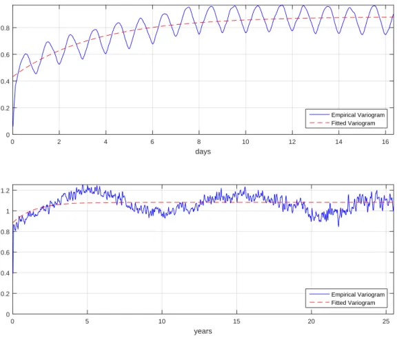
(where Vj(θ) is small). In Figure 1.1, we present the empirical and the fitted variogram
for the S&P 500, using the discrete model described in Section 2.2. The dashed line is
a fitted exponential obtained by nonlinear weighted least-squares regression. It is worth
mentioning that, if the variograms in Figure1.1 were flat, we would conclude there is no
fast and/or slow time scale on the S&P 500 index.
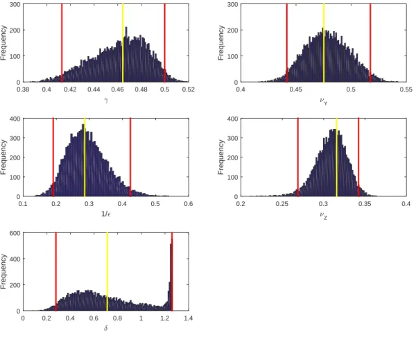
To obtain the sample distribution of the estimated parameters, we bootstrap the pairs of residuals of the nonlinear regressions solved to obtain the variograms given by Equations
(1.27) and (1.28). We use the circular block bootstrap ofPolitis and Romano(1992), with
10,000 bootstrap samples. The block size was chosen according to the procedure
devel-oped by Politis and White (2004). Table 1.1 presents the estimated values and standard
deviations for the parameters, as well as the 95% bootstrapped confidence interval. The
4
days
0 2 4 6 8 10 12 14 16
0 0.2 0.4 0.6 0.8
Empirical Variogram Fitted Variogram
years
0 5 10 15 20 25
0 0.2 0.4 0.6 0.8 1 1.2
Empirical Variogram Fitted Variogram
Figure 1.1: The empirical variogram for the S&P 500 volatility process
sample distribution of the estimated parameters is shown in Figure 1.2.
Table 1.1: Summary statistics of the estimates of the model variogram (1.26).
Parameter Estimate Mean Std Dev 95% Confidence Interval
LB UB
γ 0.4643 0.4614 0.0233 0.4128 0.4998
νY 0.4752 0.4783 0.0199 0.4417 0.5174
1/ǫ 0.2860 0.2933 0.0600 0.1908 0.4240
νZ 0.3158 0.3091 0.0186 0.2690 0.3421
δ 0.7114 0.7321 0.3104 0.2775 1.2590
Note: This table presents the summary statistics of the estimated parameters of the S&P
500 variogram given by Equation (1.26). The parameters were estimated by using weighted least-squares regression. We fit Equation (1.27) using 5-min data and Equation (1.28) using 5-day data simultaneously by performing the procedure described in Section1.2.3. The mean, standard deviation, and 95% confidence interval of each parameter were obtained by using a circular block bootstrap with 10,000 bootstrap samples. LB indicates the lower bound of the confidence interval, whereas UB indicates the upper bound.
In Table 1.1, observe that the estimate of the fast time scale, 1/ǫ, is 0.286, with
standard deviation equal to 0.023, meaning an average decoupling time of 3.497 days,
with a 95% confidence interval [2.358,5.241]. The estimated slow time-scale, δ, is 0.711,
which corresponds to a mean-reversion time of 16.868 months, with a confidence interval
[9.531,43.243]. Notice that these speeds of mean reversion indicate that the S&P 500
volatility process is driven by a fast reverting diffusion and a slowly varying
mean-reverting process. The volatility of the invariant distribution of the OU process Y was
estimated to be 0.475, while the volatility of the OU processZ was estimated to be 0.316.
Note the oscillatory nature of the variograms in Figure 1.1. This characteristic is
related to intra-day variation of volatility, and this was already noticed in Fouque et al.
(2000). For a discussion of this cycles from an implicit-volatility viewpoint, see Fouque
et al.(2004).
1.3.3
Calibration Results
In this section, we report the results of the calibration of the group market parameters to the market implied volatility data on a specific day, following the procedure outlined in Section 2.4. Our goal is to demonstrate the improvement in fit of the models’s predicted
.
0.38 0.4 0.42 0.44 0.46 0.48 0.5 0.52
Frequency
0 100 200 300
8Y
0.4 0.45 0.5 0.55
Frequency
0 100 200 300
1/0
0.1 0.2 0.3 0.4 0.5 0.6
Frequency
0 100 200 300 400
8Z
0.2 0.25 0.3 0.35 0.4
Frequency
0 100 200 300 400
/
0 0.2 0.4 0.6 0.8 1 1.2 1.4
Frequency
0 200 400 600
Figure 1.2: Bootstrap distributions of the sample parameters
In order to do that, we consider three different models:
• Model 1: in this model, we assume that the volatility is driven by a single
mean-reverting OU process, Zt, fluctuating on a slow time scale;
• Model 2: at the opposite extreme, in this model we assume that the volatility process
is only driven by a fast mean-reverting OU process, Yt;
• Model 3: in this model, we assume that the volatility is driven by two different
factors, one fluctuating on a fast time scale, Yt, and a other fluctuating on a longer
time scale, Zt.
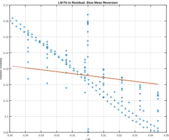
We first look at the performance of Model 1, which considers only a slow volatility
factor. In Figure 1.3a, we show the results of the calibration using only the slow-factor
approximation given by Equation (1.39), which corresponds to assuming ǫ = 0. In line
with the findings of Fouque, Papanicolaou, Sircar, and Solna (2011), we observe that
Model 1 fails to capture the range of maturities. In Figure1.3b, we look at the performance
of Model 2, which uses only the fast-factor approximation given by Equation (1.38).
Again, note that Model 2 fails to capture the range of maturities.
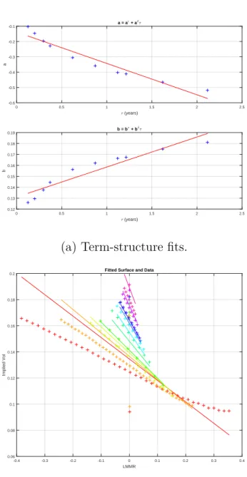
Finally, in fitting the Model 3, which uses the two-factor volatility approximation
(1.32), we follow the two-step procedure of Fouque, Papanicolaou, Sircar, and Solna
(2011). First, we fit the skew to obtain ˆai and ˆbi for different maturities τi. In the
second stage, these estimates are then fitted to an affine function of τ to give estimates
of b∗, bδ, aǫ, and aδ. A plot of this second term-structure fit on November 03, 2015, is
shown in Figure1.4a along with the calibrated multiscale approximation (1.32) to all the
data on November 03, 2015 in Figure1.4b.
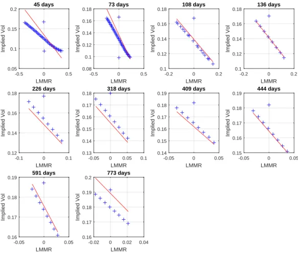
In Figure 1.4b, note that the ability of Model 3 to capture the range of maturities is
much improved when compared to Models 1 and 2. Thus, the two-scale volatility model with its additional parameters performs better than either of the one-scale models.
Table1.2 reports the estimated parameters of the correction to the Black-Scholes price
for each one of the three models presented in this section. Observe that in the regime
where our approximation is valid, the parameters aǫ,aδ, andbδ are expected to be small,
while b∗ is the leading-order magnitude of volatility. The first parameter, σ∗, can be
interpreted as an indicator of the “average” S&P 500 volatility level. Here,r is the
risk-free rate, which we assume to be known and constant. Throughout our analysis, we use
r= 0.34%, which is the value of the interest rate released by the Federal Reserve (FED)
LM
-0.05 -0.04 -0.03 -0.02 -0.01 0 0.01 0.02 0.03 0.04 0.05
Implied Volatility
0.09 0.1 0.11 0.12 0.13 0.14 0.15 0.16
0.17 LM Fit to Residual: Slow Mean Reversion
(a) τ-adjusted implied volatility I −bδτ.
LMMR
-0.4 -0.3 -0.2 -0.1 0 0.1 0.2 0.3 0.4
Implied Volatility
0.08 0.1 0.12 0.14 0.16 0.18
0.2 Pure LMMR Fit: Fast Mean Reversion
(b) S&P 500 implied volatilities.
Figure 1.3: Data and calibrated fit on November 03, 2015.
In Figure (a), we plot the maturity adjusted implied volatility as a function of the log-moneyness, LM. The plus signs are from S&P 500 data and the lineσ∗+aδ(LM) shows the result using the estimated parameters from only a slow factor fit. In figure (b), we present the S&P 500 implied volatilities as a function of the LMMR. The plus signs are from S&P 500 data, and the line
= (years)
0 0.5 1 1.5 2 2.5
a
-0.6 -0.5 -0.4 -0.3 -0.2
-0.1 a = a
0
+ a/ =
= (years)
0 0.5 1 1.5 2 2.5
b
0.12 0.13 0.14 0.15 0.16 0.17 0.18
0.19 b = b
$ + b/
=
(a) Term-structure fits.
LMMR
-0.4 -0.3 -0.2 -0.1 0 0.1 0.2 0.3 0.4
Implied Vol
0.06 0.08 0.1 0.12 0.14 0.16 0.18
0.2 Fitted Surface and Data
(b) Data and calibrated fit.
Figure 1.4: Data and calibrated fit on November 03, 2015 (slow scale).
LMMR
-0.5 0 0.5
Implied Vol
0.05 0.1 0.15
0.2 45 days
LMMR
-0.5 0 0.5
Implied Vol 0.08 0.1 0.12 0.14 0.16
0.18 73 days
LMMR
-0.2 0 0.2
Implied Vol
0.1 0.12 0.14 0.16
0.18 108 days
LMMR
-0.2 0 0.2
Implied Vol
0.1 0.12 0.14 0.16
0.18 136 days
LMMR
-0.1 0 0.1
Implied Vol
0.12 0.14 0.16
0.18 226 days
LMMR
-0.05 0 0.05 0.1
Implied Vol 0.13 0.14 0.15 0.16 0.17
0.18 318 days
LMMR
-0.05 0 0.05
Implied Vol 0.14 0.15 0.16 0.17 0.18
0.19 409 days
LMMR
-0.05 0 0.05
Implied Vol
0.15 0.16 0.17 0.18
0.19 444 days
LMMR
-0.05 0 0.05
Implied Vol
0.16 0.17 0.18
0.19 591 days
LMMR
-0.02 0 0.02 0.04
Implied Vol
0.16 0.17 0.18 0.19
0.2 773 days
Figure 1.5: Implied volatility fit of S&P 500 index options on November 03, 2015.
Table 1.2: Estimated values of the group market parameters
σ∗ aǫ aδ b∗ bδ V0δ V1δ V3ǫ
Model 1 0.1257 -0.1223 0.0308 0.0313 -0.0019
Model 2 0.1434 -0.1192 0.1426 -0.0004
Model 3 0.1318 -0.1383 -0.2049 0.1311 0.0274 0.0285 -0.0035 -0.0003
Note: In this table, we report the estimated parameters from the fit of implied volatilities
to log-moneyness to maturity ratio for Models 1 to 3 on November 03, 2015. For Models 1 and 2, we fit respectively Equations (1.38) and (1.39) to data using ordinary least-squares regression. The estimated parameters for Model 3 result from the fit of Equation (1.32) to data following the 2-step procedure suggested by Fouque, Papanicolaou, Sircar, and Solna
(2011). The last three columns were obtained through the inversion of Equations (1.34) to (1.37).
To measure the quality of the price forecasts, we use the root mean square error
(RMSE). Table1.3reports the RMSE for Black-Scholes prices and total (corrected) prices.
Panel A reports the RMSE for Black-Scholes prices obtained by using the volatilities
derived from each stochastic volatility model (Models 1 to 3).5 Panel B presents the
RMSE between total prices and observed prices. Among all the alternative models, the one that achieves the smallest RMSE is the Black-Scholes Model 2. Overal, there is no model that dominates the others in terms of RMSE.
In Table1.4, we present the average ratio between the correction termP1 and the total
price P∗ given in Equation (1.20), in percentage terms. Note that the correction is, in
average, greater than 8% of the total price for all the models considered, indicating that for a market maker, for instance an investment bank, a robust model that accounts for volatility randomness should be considered in order to price and hedge European options.
5
Table 1.3: Root mean square error (RMSE)
Call Put
Panel A: RMSE of Black-Scholes prices
BS Model 1 10.8640 28.4907
BS Model 2 9.4018 30.3767
BS Model 3 9.7651 34.9973
Panel B: RMSE of corrected prices
Model 1 10.1323 28.7596
Model 2 18.0968 15.7600
Model 3 18.6714 15.1292
Note: This table presents the root mean square error (RMSE) between estimated prices and observed prices. Panel A reports the RMSE between Black-Scholes prices and observed prices when Black-Scholes prices are estimated by using the volatilities derived from each model of first-order correction. Panel B presents the RMSE between final prices (corrected) and observed prices.
Table 1.4: Ratio between the correction term P1 and the total price P∗
Call Put
Model 1 19.7600 8.6089
Model 2 9.5989 12.9864
Model 3 63.9428 19.3682
Note: This table presents the ratio between the correction term P1 and the total price P∗
given in Equation (1.20). All values are reported in percentage terms.
1.3.4
Numeric Examples
The goal of this section is to present a numerical experiment using synthetic data (i.e.,
synthetic option prices) in order to show the validity of the asymptotic theory ofFouque,
We will denote asN∗ the true number of volatility scales that generate the data, while
N will be the value with which we do the estimation. In this paper, we will generate
synthetic data assuming that N∗ = 2 under five possible parameter settings. Relevant
parameters and functions for the two-factor stochastic volatility model (1.3) are specified
in Table 1.5. Most parameters are chosen roughly as the same order as found in Fouque
and Han (2004), and instant correlation coefficients ρ1 and ρ2 are chosen to be negative.
The volatility risk prices Λ1 and Λ2 are chosen as zeros for simplicity. The volatility
functionf is chosen as a cut-off exponential function, which is referred as a log-AR type
model in econometric literature. Initial conditions and option parameters are also given
in Table 1.5. The price computations will be done with various values of the time scales
parametersα ≡1/ǫ and δ.
In the estimation, we will useN = 1 (Model 1 and Model 2) or N = 2 (Model 3). For
each combination of input parameters we generate 1500 sample paths for the returns and
volatilities by using the stochastic volatility model (1.3). Each path is simulated for 5000
periods by using an Euler scheme with time-step size ∆t = 10−4. To generate a
cross-section of options prices, we consider options with maturities that range from 2 months
up to 36 months (τ ∈ {2,3,6,12,18,24,36}). For each maturity, we simulate option
prices for 21 different strike prices. Here, strike prices are chosen so that the moneyness
is between 0.95 and 1.05, i.e., K ∈ [0.95S0,1.05S0], where S0 is the initial price of the
underlying. Thus, our final dataset will be composed by 147 option prices.
Table 1.5: Parameters and initial conditions used in the two-factor stochastic volatility
model (1.3).
r my mz νy νz ρ1 ρ2 ρ12 Λy Λz f(y, z) Y0 Z0 S0
0.1 -0.8 -0.8 0.5 0.8 -0.02 -0.2 0 0 0 exp(y+z) -1 -1 55
In Table 1.6, we present the RMSE for Black-Scholes prices and final prices. Panel
A reports the RMSE for Black-Scholes prices obtained by using the volatilities derived from each model of first-order correction. Panel B presents the RMSE between final prices (corrected) and “true” prices. True prices are obtained as a result of Monte Carlo
simulations with 1500 sample paths generated for each set of parameters. In Table 1.7,
we present the average ratio between the correction termP1 and the total priceP∗ given
in Equation (1.20), in percentage terms.
In Table 1.6, note that the RMSE of all models decrease from regime (1) through
Table 1.6: Root mean square error (RMSE)
Call Put Call Put Call Put Call Put Call Put
(1) α= 100, δ= 0.01 (2) α= 50, δ= 0.05 (3) α= 20, δ = 0.1 (4)α= 10, δ= 0.1 (5) α= 5, δ= 1
Panel A: RMSE of Black-Scholes prices
BS Model 1 2.1727 3.3384 1.6911 2.3190 1.3232 1.3786 1.1821 0.8771 1.3720 1.1163 BS Model 2 2.8808 3.1327 2.3107 2.1525 1.8103 1.2445 1.5545 0.7886 1.8427 1.0008 BS Model 3 2.4028 3.3524 1.8757 2.3734 1.4728 1.3974 1.2955 0.8814 1.5339 1.0833
Panel B: RMSE of corrected prices
Model 1 2.0281 3.5910 1.8645 2.3272 1.5350 1.3072 1.2869 0.8417 1.5181 1.0767 Model 2 2.4438 3.0054 1.9439 2.0148 1.4785 1.1618 1.2265 0.7684 1.4424 0.9628 Model 3 2.1615 3.9698 2.0887 2.4612 1.6309 1.3309 1.2766 0.8240 1.5325 1.0286
Note: This table presents the root mean square error (RMSE) between estimated prices and true prices. Panel A reports the RMSE between
Black-Scholes prices and observed prices when Black-Scholes prices are estimated by using the volatilities derived from each model of first-order correction. Panel B presents the RMSE between final prices (corrected) and observed prices.
Table 1.7: Ratio between the correction term P1 and the total price P∗
Call Put Call Put Call Put Call Put Call Put
(1)α = 100, δ= 0.01 (2) α= 50, δ= 0.05 (3) α= 20, δ = 0.1 (4) α= 10, δ = 0.1 (5) α= 5, δ = 1
Model 1 78.3991 26.8277 29.4919 23.1520 14.3242 19.0513 8.1298 13.1969 10.6647 14.9557 Model 2 12.2209 17.1074 9.6905 48.6363 7.7229 24.0813 7.4471 29.3634 8.0624 25.8560 Model 3 304.4928 76.9366 101.4560 38.1709 30.8587 26.6432 14.0525 20.9301 17.3343 22.0662
Note: This table presents the ratio between the correction term P1 and the total price P∗ given in Equation (1.20). All values are reported in
percentage terms.
1.3.5
Application: Pricing an Exotic Derivative
In this section, we present an application of the model for pricing a binary or digital
option with no exercise option, using the calibration obtained in Section1.3.3 for options
in and close to the money.
Consider a cash-or-nothing call that pays a fixed amount Q on the dateT if XT > K,
and zero otherwise. Its payoff function is
h(x) = Q1{x>K}, (1.42)
where1A is the indicator function of a set A.
According to the perturbation theory developed in Fouque, Papanicolaou, Sircar, and
Solna(2011), the stochastic volatility-corrected price is given by
˜
P(t, x, z) = P0(t, x, z) +P1(t, x, z) =Qe−r(T−t)N(d2) +P1(t, x, z), (1.43)
where
P1(t, x, z) = (T −t) V0δ
∂ ∂σ +V
δ
1D1
∂ ∂σ
!
+V3ǫD1D2
!
PBS∗ , (1.44)
and P∗
BS =Qe−r(T−t)N(d2).
1.4
Concluding Remarks
In this paper, we present an empirical study of the American equity market, adopting
three specifications of the stochastic volatility model proposed inFouque, Papanicolaou,
and Sircar (2000). The main idea of this asymptotic model is to use perturbation tech-niques to correct constant volatility models in order to capture the effects of stochastic volatility. From the theoretical viewpoint, the model is consistently built under the as-sumptions of no-arbitrage and of the appearance of large and small time scales in the stochastic volatility models. From the practical viewpoint, it is parsimonious and easy to calibrate.
FollowingFouque, Papanicolaou, and Sircar (2000), we derive a first-order asymptotic
In the first part of our empirical study, we used S&P 500 data to show that the volatility
process of this index is driven by two diffusions: one fast mean-reverting,Yt, and one slow
mean-reverting,Zt. We found a fast time scale of 3.5 days, and a slow time scale of 16.9
months. These time-scales are statistically significant, and therefore cannot be ignored in option pricing and hedging. Thus, we can conclude that the American market is under a fast mean-reverting regime, but it is also under a slow mean-reverting regime.
Finally, in order to test the robustness of these models to different specifications, we simulate options prices using Monte Carlo simulations. We assume that the true volatility is driven by two diffusions. After that, we derived three different first-order price approximations. We did not find any evidence that these asymptotic models perform better, in terms of RMSE, than the Black-Scholes model.
However, there are many possible limitations in our analysis. First, we did not use any variance reduction technique in the Monte Carlo simulations. Second, due to computa-tional issues, we simulated a small number trajectories in our numerical exercise. Finally, we did not compare the performance of these models with other models typically used in the literature, like the Heston model, for instance.
Although theFouque, Papanicolaou, Sircar, and Solna(2011)’s models do not perform
well in terms of RMSE between corrected prices and true prices, our paper is the first
one to test the performance of three different specifications of theFouque, Papanicolaou,
Sircar, and Solna (2011)’s models. This paper gives one possible direction for further research on the improvement of these asymptotic models.
Appendix
1.A
Properties of the Variogram Estimator
In this section, we will study some properties of the variogram estimator given by
Equation (1.26). In order to do that, consider the following lemmas:
Lemma 1. Let s < t, then
Eh(Yt−E[Yt]) (Ys−E[Ys]) i
=νY2e−α(t−s)1−e−2αs, (1.45)
Eh(Zt−E[Zt]) (Zs−E[Zs]) i
Proof.
Eh(Zt−E[Zt]) (Zs−E[Zs]) i
=E νY
√
2α
Z t
0 e
−α(t−u)dW(1)
u νZ √
2α
Z s
0 e
−α(s−u)dW(1)
u
= 2ανY2e−α(t+s)E
Z t
0 e
αudW(1)
u
Z s
0 e
αu)dW(1)
u
= 2ανY2e−α(t+s)E
Z s
0 e
αudW(1)
u
Z s
0 e
αudW(1)
u +
+ 2ανY2e−α(t+s)E
Z t s e
αudW(1)
u
Z s
0 e
αudW(1)
u
= 2ανY2e−α(t+s)E
Z t
0 e
αudW(1)
u
Z s
0 e
αudW(1)
u
= 2ανY2e−α(t+s)E
Z t
0 e
αudW(1)
u 2
= 2αν2
Ye−α(t+s)E Z t
0 e
2αudt2
=νY2e−α(t+s)(e2αs−1)
=νZ2e−δ(t−s)1−e−2δs.
Similarly, we can get (1.45).
By using the previous Lemma, we can conclude that
Ehlogf1( ¯Yj) logf1( ¯Y0)
i
≈νY2e−αj∆t,
Ehlogf1( ¯Y)2
i
≈νY2.
(1.47)
Similarly, we have
Ehlogf1( ¯Zj) logf1( ¯Z0)
i
≈νZ2e−αj∆t,
Ehlogf1( ¯Z)2
i
≈νZ2, (1.48)
where ¯Y and ¯Z denote the asymptotic distributions of the OU processes given by (1.1).
Lemma 2. For the model presented in this paper, if s < t, then
Eh(Yt−E[Yt]) (Zs−E[Zs]) i
= 2
√ α√δ
α+δ ρ˜12νYνZ
e−α(t−s)−e−αte−δs. (1.49)
Otherwise, if s > t,
Eh(Yt−E[Yt]) (Zs−E[Zs]) i
= 2
√ α√δ
α+δ ρ˜12νYνZ
Proof. Suppose thats < t, then
Eh(Yt−E[Yt]) (Zs−E[Zs]) i
=E νY
√
2α
Z t
0 e
−α(t−u)dW˜(1)
u νZ √
2δρ˜12
Z s
0 e
−δ(s−u)dW˜(1)
u
+E νY
√
2α
Z t
0 e
−α(t−u)dW˜(1)
u νZ √
2δ√1−ρ˜12
Z s
0 e
−δ(s−u)dW˜(2)
u
=E νY
√
2α
Z s
0 e
−α(t−u)dW˜(1)
u νZ √
2δρ˜1,2
Z s
0 e
−δ(s−u)dW˜(1)
u
+E νY
√
2α
Z s
0 e
−α(t−u)dW˜(1)
u νZ √
2δ√1−ρ˜12
Z s
0 e
−δ(s−u)dW˜(2)
u
=√2ανY
√
2δνZρ˜12e−αte−δs
Z s
0 e
(α+δ)udu
= 2
√ α√δ
α+δ νYνZρ˜12e
−αte−δs
e(α+δ)s−1
= 2
√ α√δ
α+δ ρ˜12νYνZ
e−δ(s−t)−e−αse−δt.
By following Fouque, Papanicolaou, Sircar, and Solna (2011) and using the previous
Lemma, we get
Ehlogf1( ¯Y) logf2( ¯Z)
i
≈ 2 √
α√δ
α+δ ρ˜12νYνZ, (1.51)
Ehlogf1( ¯Yj) logf2( ¯Z0)
i
≈ 2 √α√δ
α+δ ρ˜12νYνZe
−αj∆t, (1.52)
Ehlogf1( ¯Y0) logf2( ¯Zj)
i
≈ 2 √α√δ
α+δ ρ˜12νYνZe
−δj∆t. (1.53)
Proposition 1.
En(Fn+j−Fn)2 o
≈2c2Y + 2νY2(1−e−αj∆t) + 2νZ2(1−e−δj∆t)+
+4
√α√δ
α+δ ρ˜12νYνZ
2−e−αj∆t−e−δj∆t.