Barriers to entry in monopoly markets: automobile distribution in Brazil

B

ARRIERS TO ENTRY IN MONOPOLY MARKETS

:

AUTOMOBILE DISTRIBUTION IN

B

RAZIL

S

G

F

G

Novembro

de 2006

T

T

e

e

x

x

t

t

o

o

s

s

p

p

a

a

r

r

a

a

D

D

i

i

s

s

c

c

u

u

s

s

s

s

ã

ã

o

o

B

:

B

Sergio Goldbauma

Fernando Garciab

R

O objetivo deste trabalho é analisar os efeitos da entrada de uma segunda concessionária de automóveis em mercados previamente monopolizados. Para tanto, construiu-se um banco de dados com a localização de concessionárias de automóveis em microrregiões e características demográficas e econômicas destas microrregiões. A partir desse banco de dados e de modelos de escolha binária, foram identificadas variáveis que condicionam a existência e o número de concessionárias em microrregiões. Utilizando-se de um modelo adaptado de Bresnahan e Reiss (1990), foram estimados os custos fixos de entrada de concessionárias em mercados monopolizados. Os resultados obtidos sugerem que as barreiras à entrada não são significativas, o que aumenta a probabilidade de que a cláusula de exclusividade nos contratos de concessão não cause danos à concorrência no mercado brasileiro de distribuição de automóveis.

P

Defesa da Concorrência, Restrições Verticais, Barreiras à entrada, Distribuição de

Automóveis

a

Fundação Getúlio Vargas – SP, [email protected].

b

C

JEL

L42, L62, L81

A

This paper investigates the effects of new automobile dealers’ entry in previously monopolized markets. To do so, we have used data on both the location of automobile dealers, and automobile demand and supply variables. First, we identify relevant variables which influence the existence and the number of automobile dealers in a geographical area. Then, using a model adapted from Bresnahan and Reiss (1990), we estimate the fixed costs of auto dealers and the marginal effect of the market size on the variable profit. The estimated results suggest that the fixed costs of entry of a second automobile dealer seem to be significantly lower than the fixed costs of entry of the first one and that the increase in the profit margin resulting from product differentiation more than offsets its decrease resulting from competition. This conclusion increases the probability that the clause of exclusivity present in concession contracts does not harm the competition in the Brazilian automobile distribution market.

K

W

Os artigos dos Textos para Discussão da Escola de Economia de São Paulo da Fundação Getulio Vargas são de inteira responsabilidade dos autores e não refletem necessariamente a opinião da

FGV-EESP. É permitida a reprodução total ou parcial dos artigos, desde que creditada a fonte.

1

1

.

.

I

I

n

n

t

t

r

r

o

o

d

d

u

u

c

c

t

t

i

i

o

o

n

n

:

:

o

o

b

b

j

j

e

e

c

c

t

t

i

i

v

v

e

e

a

a

n

n

d

d

r

r

e

e

c

c

e

e

n

n

t

t

h

h

i

i

s

s

t

t

o

o

r

r

y

y

o

o

f

f

t

t

h

h

e

e

r

r

e

e

l

l

a

a

t

t

i

i

o

o

n

n

s

s

h

h

i

i

p

p

b

b

e

e

t

t

w

w

e

e

e

e

n

n

a

a

u

u

t

t

o

o

d

d

e

e

a

a

l

l

e

e

r

r

s

s

a

a

n

n

d

d

m

m

a

a

n

n

u

u

f

f

a

a

c

c

t

t

u

u

r

r

e

e

r

r

s

s

.

.

This paper investigates the existence of possible barriers to entry imposed on a second dealer in markets monopolized by a dealer of a specific brand, based on a model adapted from Bresnahan and Reiss (1990) and on a database especially constructed for this exercise.

During the nineties, we have witnessed a growing tension between auto manufacturers and retail dealers in Brazil, which resulted in a preliminary investigation by the Brazilian antitrust authority, CADE,1 about manufacturers’ allegedly restrictive practices imposed on the dealers.2 According to Graph 1, the number of auto-dealers in Brazilian market increased from 2,604 in 1990 to 2,996 in 1997, then decreased to 2,646 in 2004; the ratio between domestic wholesales and the number of auto dealers increased from 274 in 1990 to 649 in 1997, then decreased to 597 in 2004.3

1

CADE, the Brazilian antitrust agency, stands for the Portuguese acronym of Administrative Council for the Economic Defense.

2

It is the preliminary investigation no. 08012.000487/00-40, of 2001. Please see Andrade and Alves (2001).

3

Graph 1: Brazil, number of auto-dealers and domestic wholesales per auto-dealers, 1978-2004.

390 390 374

217

262 280 264 314 357 234 297 293 274 299 282 426 519 630 624 649 517 440 516 569 529 523 597 2496 26012621 2672 2641 2601 2562 2433 2427 2484 2518 2601 2604 2643 2708 2654 2689 2743 2774 2858 2888 2.814 2.794 2733 2646 2971 2996 2000 2100 2200 2300 2400 2500 2600 2700 2800 2900 3000 19 78 19 79 19 80 19 81 19 82 19 83 19 84 19 85 19 86 19 87 19 88 19 89 19 90 19 91 19 92 19 93 19 94 19 95 19 96 19 97 19 98 19 99 20 00 20 01 20 02 20 03 20 04 0 100 200 300 400 500 600 700 800 900 1000

domestic wholesale per auto dealer (right axis) Auto-dealers

Source: based on ANFAVEA’s data (ANFAVEA, 2005)

This tension can be associated to changes in the automobile retail business environment, which was influenced by a combination of two factors. The first is the technological development of automobiles, which reduced the importance of after-sales service and increased the economies of scope; the second is the advent of new information technologies, which among other innovations enabled sales over the internet4. In Brazil, we have two additional factors. One is the revision of the Automobile Distribution Law (also known as “Renato Ferrari Law”) in 1990,5 which intended to allow more intraband competition among dealers, and the other is the arrival of

4

Please see, among others, the reports prepared by Price Waterhouse & Coopers (1999), McKinsey and The Economist Intelligence Unit (2000), and the Consumer Federation of América (Cooper, 2001 and 2002). In Brazil, please see also Arbix and Veiga (2003).

5

new auto makers in the second half of the 90s, which tended to increase both intrabrand as well as interbrand competition.6

Among other changes, the 1990 revision of the Ferrari Law revoked Article 14, which fixed the dealers’ margins; in Article 5, which governed dealers’ activities, it replaced the term “assigned region” with the term “operating area”, in practice allowing consumers to buy their new vehicles wherever they wished; on the other hand, the 1990 revision preserved the principle of exclusive distribution, which prohibited dealers from selling new autos manufactured by other makers (Article 3). Also, the partially changed Article 5 of the Ferrari Law has maintained “minimum distances between dealers of the same maker, established according to market potential criteria”. In the USA, the pertinence of these two vertical restrictions – exclusive distribution and territory restriction – still imposed by some states, has been challenged by some consumer organizations.7

In addition to this introduction, this paper is organized into four other sections. The second one briefly describes empirical studies of vertical competition issues found in automobile distribution. The third one discusses the Bresnahan and Reiss (1990) model. The fourth section describes the database constructed for this paper and brings estimated results for the Brazilian market. Finally, the last section summarizes the main conclusions and discusses the implications and limitations of the findings.

2

2

.

.

V

V

e

e

r

r

t

t

i

i

c

c

a

a

l

l

r

r

e

e

s

s

t

t

r

r

i

i

c

c

t

t

i

i

o

o

n

n

s

s

i

i

n

n

a

a

u

u

t

t

o

o

m

m

o

o

b

b

i

i

l

l

e

e

d

d

i

i

s

s

t

t

r

r

i

i

b

b

u

u

t

t

i

i

o

o

n

n

:

:

a

a

s

s

u

u

m

m

m

m

a

a

r

r

y

y

o

o

f

f

s

s

o

o

m

m

e

e

e

e

m

m

p

p

i

i

r

r

i

i

c

c

a

a

l

l

s

s

t

t

u

u

d

d

i

i

e

e

s

s

.

.

Among empirical studies on the competition aspects associated to automobile distribution and to the relationship between dealers and manufacturers, one can find the classic study carried out by B. P. Pashigian (1961), The Distribution of Automobiles, an Economic Analysis of the Franchise System, and Two Studies in Automobile Franchising, by H. O. Helmers, C. N.

6

Goldbaum (2005).

7

Davisson and H. F. Taggart (1974). More recently we have Franchise Regulation: an Economic Analysis of State Restrictions on Automobile Distribution, by Richard L. Smith II (1982); The effect of State Entry Regulation on Retail Automobile Markets, by R. P. Rogers (1986); and two studies by T. Bresnahan and Peter C. Reiss: Dealer and Manufacturer Margins, of 1985, and Entry in Monopoly Markets, of 1990.

The Pashigian (1961) study is the most comprehensive. In addition to describing the relationship between dealers and manufacturers from a theoretical standpoint and detailing the auto distribution industry in the USA, the author suggests instruments to estimate the form of the dealers’ long-term cost function, in order to measure the occurrence of economies of scale in this activity. According to this author, knowing the extent of the economies of scale in automobile distribution would help establish, at least in part, the number of dealers that could operate in a given market, and consequently help us find out if competition among established dealers would take place on a price or non-price basis (e.g., services). Most importantly, it would also help to measure how open the industry would be to an arriving manufacturer. To determine how quantitatively important are barriers to entry represented by economies of scale in distribution, the author suggests a method to measure the relationship between the unit costs incurred by dealers selling vehicles and by manufacturers manufacturing them.

Pashigian (1961) concluded that economies in distribution apparently extended beyond the point where economies of manufacturing had been exhausted, which would mean a substantial barrier to entry for new manufacturers.8 When faced with the argument that new manufacturers (such as Volkswagen and Renault) enjoyed an easy and successful entrance into the US market in the late 50s and early 60s, a development which would disprove his analysis,

8

the author simply replied that the US manufacturers at that time had not perceived a change in the tastes of domestic consumers (Pashigian, 1961, p. 240).

Smith II (1982) describes the dealer system used for auto distribution in the USA in the early 80s, pointing out the manufacturers’ need to control distribution. The author also built a model to test the hypothesis that government regulation tended to give existing dealers power over the local market by protecting them. To do so, Smith II (1982) estimated the optimum number of dealers per state, considering aspects that affected demand (such as the number of driver licenses, per capita income, driver density in the region, and unobservable license price) and supply (including, among other variables, those representing regulatory restrictions of the different US states), from 1954 to 1975. The author’s analysis suggests that government regulation apparently increased the dealers’ market power, to the loss of consumer welfare.

Bresnahan and Reiss (1985) describe some “intriguing questions” seen in the US industry, such as the fact that the ratio between dealer margins and manufacturer margins is independent of the size of the vehicle and its price-elasticities and cross-elasticities. Based on the analysis of successive monopolies, the authors show that the ratio between the dealers’ and manufacturers’ margins is equal to the ratio between the slopes of the dealers’ and manufacturers’ demand curves. Bresnahan and Reiss (1985) defend four propositions:

i. In a price arrangement between the manufacturer and the dealer, involving only one product, if the demand curve is strictly convex (concave), the dealer’s margin on unit costs will be greater (lesser) than half the manufacturer’s margin.

ii. In a one-product price arrangement between the manufacturer and the dealer, the ratio between the dealer’s and the manufacturer’s margins is equivalent to the change in the dealer price when the manufacturer changes the wholesale price (the dealer’s unit cost), or when the dealer’s sale cost changes, i.e.,

(

)

( )

( )

s s P w

w P m

w

s w P

∂ ∂ = ∂ ∂ = −

+

− * *

* * *

iv. Finally, in a multi-product price arrangement between the manufacturer and the dealer, the ratio between the dealer’s and manufacturer’s margins for each product is determined by the quantity-elasticity of the demand curve ηi9. If the demand system is linear, the dealer’s

margins will be half of the manufacturer’s margins for each product. If a proportional increase in all quantities raises the weighted impact of Qi on the prices of all products, then the dealer’s margin on the product i will be greater than half the manufacturer’s margin.

Using data on production costs, wholesale prices, and resale costs and prices, the authors point out that more expensive models are subject to both greater discounts, on a percentage basis, as well as substantially wider margins. The authors conclude that the dealers’ margins are proportional to the manufacturers’ margins for the whole product line, and that we cannot reject the hypothesis that the ratio between the margins is equivalent to one half, a situation that implies demand locally linear curves.

Bresnahan and Reiss (1990) bring an empirical model of market concentration developed from an entry model based on the theory of games. The empirical model is built on inequality conditions that describe equilibrium strategies for entrant firms in simultaneous or sequential games. Such conditions are used to describe the entry into isolated monopoly markets. Based on estimations of the market size necessary to house one or two dealers, the authors conclude that monopolist dealers do not represent barriers to the entry of a second dealer. Moreover, the authors find that the entry of a second dealer does not provoke a significant decrease in the price-cost margin. The following section describes in more detail the model developed by the authors.

9

i is not the slope of the demand curve, but rather a local measure of the curvature of the dealer’s demand curve,

3

3

.

.

T

T

h

h

e

e

B

B

r

r

e

e

s

s

n

n

a

a

h

h

a

a

n

n

a

a

n

n

d

d

R

R

e

e

i

i

s

s

s

s

(

(

1

1

9

9

9

9

0

0

)

)

m

m

o

o

d

d

e

e

l

l

f

f

o

o

r

r

e

e

n

n

t

t

r

r

y

y

i

i

n

n

m

m

o

o

n

n

o

o

p

p

o

o

l

l

y

y

m

m

a

a

r

r

k

k

e

e

t

t

s

s

The model for entry in monopoly markets developed by Bresnahan and Reiss (1990) is based on the theory of games, and is adapted from the individual qualitative choice model for firms whose profits and costs are not observable. The main idea is that a potential entrant firm will only actually enter a monopoly market if it expects duopoly positive profits. Unlike individual models, the decisions taken by firms entering a market are interrelated and their profits depend on the decisions of the other competitors.

The authors assume the following demand function:

(

) ( )

D

Q_i = _i , (1)

where Di

(

)

variable S represents the number of representative consumers, Z represents the market conditions, and P the price of the good i. Note that Z does not include S, which means that the size of the market does not affect consumer preference. The size of the market, in turn, is a function of Y, which represents demographic variables.

On the cost side, the authors assume:

(

)

( )

( )

C_{i i}, = _{i i} + _i (2)

where Qi represents the unit sales of firm i; ci(W), the variable costs (in which the marginal cost is constant); the vector W, exogenous variables that affect the costs (such as raw material prices); and Fi(W), the fixed costs. Inverting the demand function, one can obtain the following profit function of the potential entrant firm i, which depends on its production and the production of its competitors.

(

)

[

]

i = P Z Q S −c Q −F

Π , / (3)

(

) ( )

[

]

(

) ( )

( )

N i i N

i N

i = − −

Π , , , or

(

) ( )

( )

V i

N i N

i = −

Π , (4)

where N denotes monopoly (N=M) or duopoly (N=D).

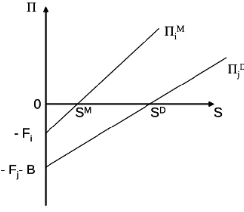
Figure 1 compares the market structure, defined by the profit of the monopoly or duopoly, to the size of the market. The curves define, in the horizontal axis market sizes that do not support any firm (between 0 and SM), one monopoly firm (between SM and SD) and two duopoly firms (to the right of SD). In this figure, SD is on the right of SM because the firm j has higher fixed costs and lower profits per buyer than firm i. Such increase in the fixed cost is the equivalent to including barriers to entry B.

Figure 1: Profit as a function of market size.

0

SM _SD

П

ПiM

ПjD

- F_i

- F_j- B

S 0

SM _SD

П

ПiM

ПjD

- F_i

- F_j- B

S

Source: Bresnahan e Reiss (1988)

While profits are not observable, the SD and SM break-even levels are. At SM, the monopolist’s profit is zero. That is, starting from equation (4):

(

)

i i M i

i M

D c P

F S

−

= (5)

(

)

= (6)

Comparing both levels of demand, we have:

(

)

(

)

F D c P D b c P S S j i M i i M i D j j D j D M + ⋅ − − − =

The first term on the right side of the equation provides VD/VM, i. e., the ratio of the derivatives of the duopoly and monopoly profits in relation to the size of the market S (variable profits).

(

)

(

)

i i M i D j j D j M D M D D c P D b c P S S V V − − − = ∂ Π ∂ ∂ Π ∂ = / / (7)

The VD/VM ratio decreases if post-entry competition increases j (i.e., if the price of the duopoly equilibrium decreases or if the production costs of firm j (i.e., cj+b) increase, which can be estimated based on the qualitative information on the profits of new entrants. Estimating VD/VMand SM/SD, the ratio of the fixed costs of new entrants:

B F F F F j i D M +

= (8)

can also be estimated.

Summing up, the ratio between the break-even points can be expressed as the product of the inverse ratio of the variable profits and the direct ratio of the entry fixed costs, i.e.:

D M M D D M F F V V S

S _{= ⋅}

which enables us to estimate the ratio between the fixed costs of entry using:

M D D M D M V V S S F F /

The Bresnahan and Reiss (1990) analysis uses variable profits and fixed costs ratios because the empirical data do not allow us to separately identify the individual components in these ratios.

The entry model described above implicitly assumes a series of assumptions. For example, it does not consider the possibility of the existing monopolist discouraging the entry of new players by reducing the monopoly price when the market size approached SD – which would imply a less steep slope of the monopolist's profits when S approached SD. Overall, it omits non-linear pricing strategies and asymmetric information, among other possibilities.

Based on this model, Bresnahan and Reiss (1990) use the firms’ equilibrium pay-off functions to formulate equations that describe optimal entry strategies. The entry is modeled as a binary decision that corresponds to two pure strategies: Ii = 1, if the firm enters, e Ii = 0, if it does not enter. Two potentially entrant firms face each other in a one-round game, in which each firm knows the strategies and payoffs of its respective competitors. The entry decision of firm 1 depends on the entry decision of firm 2, and vice-versa. Both act in a non-cooperative manner, in two possible situations, when decisions are simultaneous and when they are sequential. However, in this paper we will only detail the situation of simultaneous decisions.

a. Simultaneous decisions

The pair I*1 and I*2 forms Nash's pure strategy equilibrium if

(

)

(

)

2 1 1 * 2 * 1

1 I ,I ≥Π I ,I

Π , for I₁∈

{ }

(

)

(

)

* 1 1 * 2 * 1

2 I ,I ≥Π I ,I

Π , for I2∈

{ }

If a firm earns zero profit when opting for I = 0, then its optimum entry strategy will be the following:

(

)

0 ₂* _{1 2}* ₁

*

1 = ⇔ − Π + Π <

D M

I I

I , and

(

)

0 ₁* _{2 1}* ₂

*

0 = ⇔ − Π + Π <

D M

I I

I . (10)

Table 1 describes the other pure-strategy solutions, considering only that the duopoly profits cannot be greater than those of the monopoly.

Table 1: Results of pure strategy in a game of simultaneous decisions

0

1 < ΠM

, Π₂M <0 No entrant

0

1 > ΠD

, Π₂D >0 Duopoly

D M

1 1 >0>Π

Π , Π₂M >0>ΠD₂ Monopoly of firm 1 or 2

0

1 > ΠM

, Π₂D <0 Monopoly of firm 1

0

1 < ΠD

, Π₂M >0 Monopoly of firm 2 Source: Bresnahan and Reiss (1990)

Following Bresnahan and Reiss (1990), the first line of the table describes a situation in which no entry takes place; the second shows one in which two firms enter. The last three lines describe monopoly situations, the last two implicitly including the condition “and not any of the previous events”; the third line shows a situation in which there is no single result of pure strategy.

The presence of non-unique equilibria in theory of games models prevents the use of the standard qualitative choice models to model the entrants’ profits. To get around this problem, the authors reinterpreted the model, to include N = I1 + I2, the number of entrants. Thus, the last three lines of the table represent a single result, N = 1.

b. Treatment of unobservable data

On the other hand, to get around the problem of neither earned profits nor expected profits being observable, the authors model the firms’ profits as unobservable random variables, adding an error term in the equilibrium profit function (4). Specifically, the profit of the Nth entrant’s profit has the following form:

in which variable profits are equivalent to the sum of a measurable profit component V(⋅) and an unobservable component . Similarly, fixed costs have a measurable component F and an error term ε.

In the econometric models the authors developed, the stochastic structure of (11) was restricted because of computational and economic conditions. For example, to prevent duopoly profits from exceeding the monopoly profits with a positive probability. The authors developed three models: (i) perfectly correlated unobservable profits; (ii) correlated errors; and (iii) monopoly and duopoly errors not perfectly dependent. In this paper we opted to detail only the first model, that in which the unobservable profits are perfectly correlated. This model presupposes that all potential entrants have the same fixed costs and unobservable variable profits, i.e.: ε₁M =ε₁D =ε₂M =ε₂D and η₁M =η₁D =η₂M =η₂D. Although this error specification implies strong assumptions on the unobservable profit distribution, it presents two advantages. The first is that if the firms only have independent and identically distributed fixed costs, then the firms’ profit parameters can be estimated using an ordered probit model. Including an error term in the variable profits, we get a heteroscedastic ordered probit model, in which the variance of unobservable profits, σ_ξ2 =1+σ_η2S2, increases with the size of the market.

Thus, the probabilities associated to the observation of markets with no firms, two firms, or one firm are the following:

(

)

[

]

1

0 Z W Y

P = −ΦΠM

(

)

[

]

2 Z W Y

P =ΦΠD

2 0 1 1 P P

P = − − (12)

The model is estimated from equation (4), using data obtained from isolated markets in the USA. The specifications are summarized in equations (13), (14) and (15):

S(Y) = TOWNPOP + λ(Y) (13)

FN = γM + γDD + γWW (15)

Where TOWNPOP is the population of the central city, Y are the other demographic variables, the superscript N can be M (monopoly) or D (duopoly), D is a dummy variable for duopolies, Z is a demand conditioner vector, and W a supply conditioner vector (costs). The results obtained in the simplest model, which excludes Y, Z and W, are shown in Table 2.

As shown in Table 2, the ratio VD/VM measures the fraction by which variable profits per client decrease with the entry of a new firm. When duopolists sell the same product, VD/VM should be equal to (in the case of collusion) or less than (in the case of non-cooperative behavior) 0.5. Since the ratio VD/VM observed in Brensahan and Reiss (1990) is greater than 0.5, (in this case, VD/VM = 0.752), the authors conclude that product differentiation increased the duopoly margin more than competition was able to decrease it. Consequently, “entry by a Ford dealer into a monopoly GM market would not lower a monopoly GM dealer’s sales and variable profits by much” (Bresnahan and Reiss, 1990, p. 552).

Table 2: Bresnahan and Reiss (1990), estimations based on the ordered probit model for the number of auto dealers.

Variables Coefficients Model (1) Asymptotic standard error

V-monopoly (VM) M 0.933 (3.39)

V-duopoly (VD) M + D 0.702 (5.02)

F-monopoly (FM) γM 0.536 (1.79)

F-duopoly (FD) γM ₊ γD 1.277 (5.39)

Log likelihood -123.76

SM _{575 (188)}

SD _{1820 (166)}

SM_/SD _{0.316 (0.095)}

VD_/VM _{0.752 (0.180)}

FM_/FD _{0.419 (0.183)}

Log likelihood -123.76

Source: Adapted from Bresnahan and Reiss (1990), tables 5 and 8.

monopoly, these costs cannot be attributed to entry barriers. The estimations obtained from the sequential entry model suggested that, unlike the entry order, the fixed costs could vary, say, according to the brand.

4

4

.

.

B

B

a

a

r

r

r

r

i

i

e

e

r

r

s

s

t

t

o

o

e

e

n

n

t

t

r

r

y

y

i

i

n

n

m

m

o

o

n

n

o

o

p

p

o

o

l

l

y

y

m

m

a

a

r

r

k

k

e

e

t

t

s

s

:

:

a

a

u

u

t

t

o

o

m

m

o

o

b

b

i

i

l

l

e

e

d

d

i

i

s

s

t

t

r

r

i

i

b

b

u

u

t

t

i

i

o

o

n

n

i

i

n

n

B

B

r

r

a

a

z

z

i

i

l

l

This section analyzes the existence of barriers to entry into monopoly markets in the Brazilian auto distribution industry. To do so, we organized a database containing the location of all automobile and light commercial vehicles in Brazil in 2004, according to manufacturer and city10. This information has been crossed with the municipal characteristics, obtained from 2000 Census micro-data and aggregated into micro-regions, which, considering consumer mobility and production factors, are believed to provide a suitable analysis unit.

The 2000 Census data were considered proxies for the characteristics of the micro-regions existing in 2004. No information on dealer location was found for 2000, and the available data on micro-regions for 2004 were not as detailed as those based on the 2000 Census micro-data.

This analysis is subdivided into three sub-sections. The first analyzes the dealer location determinants in the micro-regions. The second analyzes the dealer number determinants in each micro-regions. The third uses the variables found in the previous sections to investigate the signs of the existence of barriers to entry into the auto distribution industry in Brazil, based on the Bresnahan and Reiss (1990) model.

4.1 Analysis of dealer location determinants in a micro-region.

To analyze the dealer location determinant factors, we built a binary choice model of the following type:

10

(

)

(

)

P =1| = ₀+ (A)

in which the variable y assumes the value of zero if no dealers exist in a micro-region, or the value of one, if there is at least one dealer. The independent variable vector x gathers demographic data, which condition the demand for automobiles and information on the cost of dealer installation in a micro-region.

Alternatively, the model can be read to implicitly assume the latent (unobservable) variable economic profit (y*):

ε β

β + +

= x

y* ₀ , y=1

[

]

The probability of an answer to y is:

(

) (

)

[

(

)

]

[

(

)

]

(

)

P =1| = *=0| = >− ₀ + | =1− − ₀+ = ₀+ (B)

which is the same of the model (A). In the logit model, G is a logistic function, while in the probit model, G is an accumulated standard normal distribution function. Details on the binary choice models are found in Wooldridge (2002), Griffiths et al. (1993) and Cramer (2001).

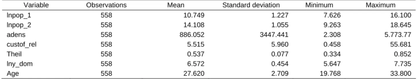
After preliminary analyses, the best results were obtained with the variables shown in Table 3 below, in which the first two are demographic variables, relative to market size; the next two are supply shifters; and the last three are demand shifters. The main statistics describing these variables are shown in Table 4.

Table 3: Variables used in binary choice models

Variables Meaning lnpop_1 Natural log of the urban population of the micro-region’s largest city.

lnpop_2 Natural log of the remaining population in the micro-region (i.e., rural population plus urban population of the other cities.

adens Inhabitants per square kilometer.

custof_rel Average wage of workers in administrative positions employed in auto retail, divided according to per capital income in each micro-region, in R$. (*)

lny_dom Natural log of average income per household, in R$. Theil Theil’s L inequality index, computed for each micro-region. Age Average age in each micro-region.

Table 4: Statistics describing independent variables used in binary choice models

Variable Observations Mean Standard deviation Minimum Maximum

lnpop_1 558 10.749 1.227 7.626 16.100

lnpop_2 558 14.108 1.055 9.263 18.645

adens 558 886.052 3447.441 2.308 5.773.77

custof_rel 558 5.515 5.960 0.458 55.681

Theil 558 0.537 0.077 0.334 0.852

lny_dom 558 6.572 0.454 5.647 7.735

Age 558 27.620 2.709 19.768 33.800

Source: Based on Census data (IBGE, 2000).

The results of the logit and probit models are shown in Table 5. In this Table we see that the demographic variables and those representing demand conditioners have positive signs, while those representing supply conditioners (costs) have negative signs. Specifically in regard to the adens (population density) variable, we believe that it is a proxy for the costs of property where the dealer is located.

Table 5: Results of binary choice models

Probit Logit Variables

Coeff. Standard

deviation dF/dx

Standard

deviation Coeff.

Standard deviation

lnpop_1 1.292(***) 0.235 0.358(***) 0,063 2.272(***) 0.427

lnpop_2 0.883(***) 0.235 0.244(***) 0,066 1.588(***) 0.419

custof_rel -0.014 0.014 -0.0038 0,004 -0.0231 0.024

adens -0.0002(***) 0.00007 -0.00006(***) 0,00002 -0.0004(**) 0.0001

lny_dom 1.713(***) 0.339 0.474(***) 0,091 2.994(***) 0.606

Theil 3.618(**) 1.453 1.002(**) 0,424 6.624(**) 2.613

Age 0.298(***) 0.047 0.083(***) 0,0142 0.543(***) 0.089

Constante -46.663(***) 4.570 -83.077(***) 8.800

Log Likelihood -119.732 -120.524

Pseudo R2 _{0.683 0.680}

N 558 558

Note: (**) significant at 5%, (***) significant at 1%.

All the variables are significant at 1%, except variables associated to income distribution (at 5%) and to labor (which is significant only at 35%). We also see no major differences between the logit and probit models, regarding the significance of the variables.

micro-region increases the probability of a dealer existing in the micro-micro-region in approximately 5%. Table 6 shows that correct percentages for both models exceed 90%, and that forecast errors are balanced.

Table 6: Correct percentages of the dealer location models

Location forecast Location forecast

Probit

0 1 Total Logit 0 1 Total

0 200 26 226 0 200 25 225

Actual Location

1 28 304 332 Actual Location 1 28 305 333

Total 228 330 558 Total 228 330 558

Correct percentage 90,3% Correct percentage 90,5%

Source: own elaboration

4.2 Analysis of dealer number determinants in a micro-region.

To analyze the determinants of the number of dealers in a micro-region, we compared the results of two models. The first was a multiple linear regression model (in which the coefficients are computed using the ordinary least squares (OLS) method) and the second with a sample selection correction (Heckit model).

The multiple linear regression model used as regressors a subset of variables identified in the previous section:

age dom

y pop

pop

q _{0 1}ln _1 ₂ln _2 ₆ln _ ₈

ln =β +β +β +β +β (C)

The sample selection correction model used all variables identified in the previous section as variables, and only the variables used in the multiple linear regression model as regressors. The variables “lnpop_3”, “custof_rel”, “adens” and “Theil” were not significant enough to be included as regressors.

[

]

Table 7: Results of the dealer number determinants per micro-region models

OLS HECKIT lnq

Coefficient Standard error Coefficient Standard error

lnpop_1 0.256 0.063 0.231 0,063

lnpop_2 0.513 0.068 0.513 0,067

lny_dom 0.626 0.098 0.580 0,100

age 0.070 0.013 0.063 0,013

_cons -15.166 0.754 -14.334 0,877

sigma 0.475 0,019

Observações 330 558 (330 selec.)

F 261.610 R2 0.763

Log likelihood -338.160

Note: All coefficients are significant at 1%.

All coefficients are significant at 1%. Particularly important is the significance of the value of the sigma coefficient, a sign of a problem in sample selection. The coefficients of the variables “lnpop_1” and “age” are those whose correction is proportionally higher.

4.3 Analysis of the importance of barriers to the entry of new dealers.

This third exercise investigates if the existence of a dealer in a micro-region represents a barrier to the entry of a new dealer in this micro-region.

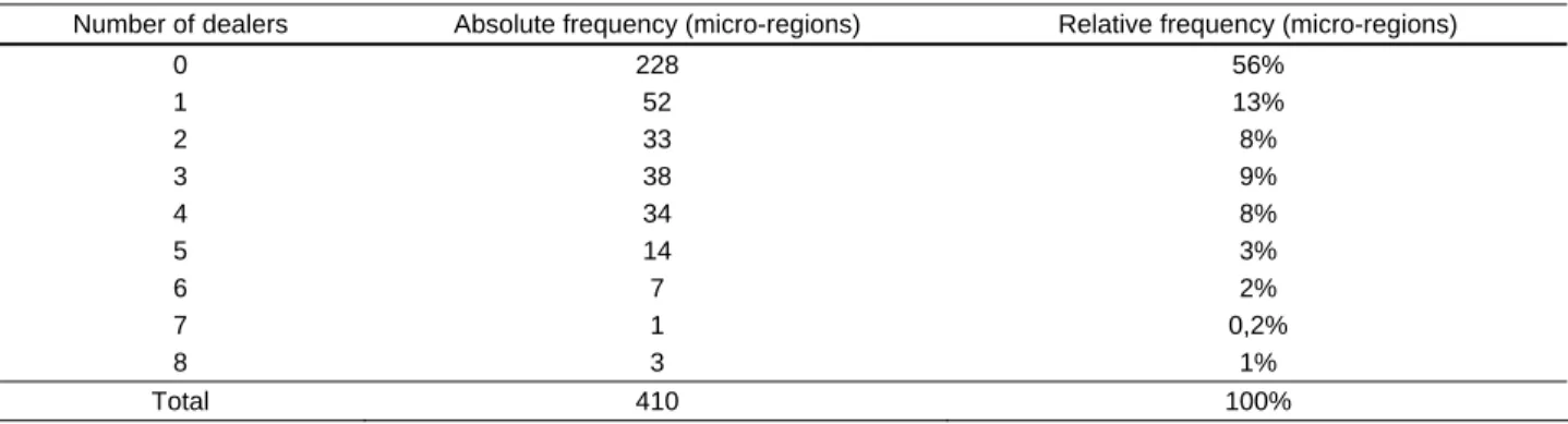
To analyze this matter, we extracted from the original database a subset of “non-shared” micro-regions, i.e., those which did not house more than one dealer of a given brand. This procedure produced a subset of 410 micro-regions, of which 228 (56% of the total) did not have any dealers, 52 (13%) had only one dealer, and up to three micro-regions (1%) had eight dealers of different brands, as shown in Table 8.

Table 8: Frequency of dealers in micro-regions, excluding shared micro-regions

Number of dealers Absolute frequency (micro-regions) Relative frequency (micro-regions)

0 228 56%

1 52 13%

2 33 8%

3 38 9%

4 34 8%

5 14 3%

6 7 2%

7 1 0,2%

8 3 1%

Total 410 100%

Source: Based on Fenabrave data.

The models built to measure the importance of barriers to the entry of new dealers is based on Bresnahan and Reiss (1990), the details of which were shown in the previous section. We used a reduced ordered probit model, in which the unobserved economic profit variable (y*) is specified according to the equation below:

adens Theil

cap y pop

y*=β₁ 1+β₂ _ +β₃ +β₄ (E)

The dependent variables are defined and characterized according to the table in Table 9. We decided to use the variables in level, no in logarithm (except for the Theil index), to enable us to directly estimate the break-even points.

Table 9: Variables used in ordered Probit model

Number of dealers Observations Variables Mean Standard deviation Minimum Maximum

pop1 39,639.39 26,620.51 2,051 262,538

y_cap 146.09 79.95 46.25 601.37

l1 0.52 0.08 0.33 0.85

0 to 2 313

adens 264.94 489.21 2.31 6,574.88

pop1 34,801.23 21,615.08 2,051 152,977

y_cap 125.67 70.64 46.25 601.37

l1 0.51 0.08 0.33 0.79

0 228

adens 234.23 332.31 2.31 2.318.85

pop1 47,371.21 27,768.71 12,665 133,738

y_cap 208.71 74.68 81.57 404.37

l1 0.56 0.08 0.45 0.85

1 52

adens 425.81 957.38 6.92 6.574.88

pop1 60,883.23 40,457.36 18,413 262,538

y_cap 188.57 82.69 80.55 368.46

l1 0.54 0.06 0.45 0.70

2 36

adens 223.62 196.87 14.13 857.99

We used five specifications, from a simpler one, in which the y* depends only on pop1, to a more comprehensive, in which all four explanatory variables comprise the model. We also tested specifications using other variables, such as average age, household income, and income of the staff employed in administrative positions at dealers.

The advantage of using the ordered probit model is that it automatically imposes an implicit presupposition in the theoretical model, namely that SM is greater than SD (i.e., the size of the market for monopoly is smaller than the size of the market for duopoly). Considering a synthetic model, the coefficients α₁ and α₂of the ordered probit model define the probabilities:

(

) (

) (

)

(

)

(

) (

) (

)

(

) (

)

(

) (

) (

)

(

)

β α β α α β α α β α α β α x x e x P x y P x y P x x x e x P x y P x y P x x e x P x y P x y P − Φ − = ≤ + ≤ = ≤ = = − Φ − − Φ = ≤ + ≤ = ≤ = = − Φ = ≤ + = ≤ = = 3 3 2 3 1 2 2 1 2 1 1 1 1 * 2 * 1 * 0 (F)

where y = 1 represents a monopoly, y = 2 a duopoly, and Φ is the normal distribution.

Table 10: Results of the ordered probit models for determining barriers to the entry of new dealers

(1) (2) (3) (4) (5) pop1 0.0000155 (***) 0.0000193(***) 0.0000196(***) 0.0000228(***) 0.0000225(***)

(2.95e-06) (3.17e-06) (3.20e-06) (3.63e-06) (3.66e-06)

y_cap 0.007032(***) 0.0065633(***) 0.0073345(***) 0.0070018(***)

(0.0009614) (0.0010124) 0.0009838 (0.001052)

Theil 1.621457 1.004655

(1.044764) (1.110083)

adens -0.0003143(**) -0.002671(*)

0.0001498 (0.0001586)

α1 1.257842 2.546358 3.354958 2.657618 3.142829

(0.1482535) (0.2488701) (0.5835764) (0.2605346) (0.599537)

α2 1.960928 3.363532 4.174723 3.484323 3.969582

(0.1684994) (0.2751392) (0.5964521) (0.2866102) (0.6112228)

Log likelihood -224.4045 -194.25998 -195.28166 -194.25998 -193.85019

Pseudo R2 0.0643 0.1900 0.1857 0.1900 0.1917

Observações 313 313 313 313 313

Note: (*): Significant at 10%. (**) Significant at 5%. (***) Significant at 1%. The numbers in parenthesis are standard deviations.

The ratio between the coefficients α₁ and α₂ and the coefficient of the variable pop1 define the scales SM and SD, i.e., the size of the urban population of the largest city in a micro-region housing zero, one or two dealers. In the models, according to Table 11, these values are approximately 81,000 and 126,000 (in the simplest model) and 140,000 and 175,000 people (in the most comprehensive model), which are relatively larger than the magnitudes actually seen. According to the database, the average urban population of the largest city in the micro-regions housing only one dealer is approximately 47,000, while in cities housing two dealers it is 60,000. Yet, if we take the comprehensive model, the proportions remain the same, i.e., SM/SD = SˆM /SˆD

≈ 0.8.

Table 11: Limit points for the ordered probit models

(1) (2) (3) (4) (5)

Monopoly (SM_{) 81,009 131,859 116,436 171,140 139,810}

(8,846) (15,645) (13,136) (32,474) (30,939)

Duopoly (SD_{) 126,289 174,176 152,655 212,957 176,589}

(16,520) (21,446) (17,903) (36,323) (34,404)

(SM/SD) 0.64 0.76 0.76 0.80 0.79

(0.04) (0.03) (0.03) (0.03) (0.04)

In addition to the values SM and SD, it is necessary to estimate proxies for the variable profits VD and VM, the derivative of unobservable profit in relation to the demographic variable. We know that in the probit model the marginal change of the latent variable in relation to changes in continuous independent variables is obtained from:

( )

_{( )}

p _{= β β}

∂ ∂

, where

( )

( )

g = is the normal distribution. (G)

In the ordered probit model, in turn, the marginal effect of the continuous independent variables is given by:

(

)

(

)

(

) (

)

[

]

β β α φ β β α φ β x x x x p x x x p x x x p j j k k j J k k J k k − − − = ∂ ∂ − = ∂ ∂ − − = ∂ ∂ −1 1 0 ) ( ) ( ) (

, for 0 < j < J (H)

We computed the marginal effects VM and VD for the mean of values x, according to the mean values of the variables shown in Table 911. The results of the marginal effects for monopoly and duopoly in the five specifications are shown in Table 12. There we see that the relation between the marginal effects in specification (4) is 0.14. In the simplest model, this relation is 1.52, while in the most comprehensive model it is 0.28.

Table 12: The marginal effect of the size of the market on the probability of entry

(1) (2) (3) (4) (5)

Monopoly (VM) 2.53e-06 2.56e-06 3.61e-06 4.23e-06 4.16e-06

(1.95e-07) (2.48e-07) (2.58e-07) (3.45e-07) (3.45e-07)

Duopoly (VD) 2.51e-06 2.24e-06 2.21e-06 2.57e-06 2.49e-06

(2.99e-07) (4.54e-07) (4.62e-07) (6.53e-07) (6.31e-07)

(VD/VM) 0.99 0.63 0.61 0.61 0.60

(0.30) (0.21) (0.20) (0.22) (0.215)

Note: the numbers in parenthesis are standard errors.

11

The theoretical model assumes, following equations (6) to (8), that the variable profit, both in a monopoly as well as in a duopoly, increases linearly with the variable representing the size of the market. In the empirical models developed in this paper, the size of the market corresponds to the variable “urban population in the largest city of the micro-region” (pop1). The marginal effects referring to the variable pop1 in monopoly and duopoly correspond, respectively, to the variables VM and VD in the theoretical model.

The ratio between these marginal effects (VD/VM) in models (1) to (5) is above 0.5, suggesting, not unlike in Bresnahan and Reiss (1990), that in the Brazilian case the increase of the margin resulting from product differentiation more than offset the decrease in the monopoly margin resulting from competition.

Following equation (8’), if we divide limit points ratio (SM/SD) by the marginal effects ratio (VD/VM), we obtain the fixed costs ratio (FM/FD). The estimations are in Table 13. In the simpler model, this ratio equals 0.65, showing that the costs of installing a second dealer would be approximately 54% higher than for the first dealer. Just as in Bresnahan and Reiss (1990), we cannot attribute this increase in costs directly to the entry barriers. It would be necessary to investigate, say, if no differences in cost associated to dealer and manufacturer brands exist.

Table 13: Ratio between fixed costs of entry in a monopoly and in a duopoly

(1) (2) (3) (4) (5)

(FM/FD) 0.65 1.20 1.31 1.26 1.32

(0.20) (0.40) (0.44) (0.44) (0.47)

Note: the numbers in parenthesis are standard errors.

5

5

.

.

S

S

u

u

m

m

m

m

a

a

r

r

y

y

,

,

c

c

o

o

n

n

c

c

l

l

u

u

s

s

i

i

o

o

n

n

a

a

n

n

d

d

i

i

m

m

p

p

l

l

i

i

c

c

a

a

t

t

i

i

o

o

n

n

s

s

This paper investigates if the existence of a dealer in a micro-region represents a barrier to the entry of a new dealer into this micro-region. To do so, we organized a database gathering information on the location of dealers according to micro-regions, based on Fenabrave data and IBGE’s 2000 Census data.

In a first phase, we identified eight variables that condition the existence and the number of dealers in a micro-region: the natural logarithm of the urban population of the largest city in a micro-region; the natural logarithm of the remaining population of a micro-region; the natural logarithm of the share of women in that population; population density (inhabitants per square kilometer); income distribution (as measured by the Theil-L); the natural logarithm of household income; wages paid to workers in administrative positions at auto dealers; and average age in each micro-region.

In a second phase, we adapted the Bresnahan and Reiss (1990) model to the Brazilian auto-distribution industry. Estimates suggest that the increase of the profit margin resulting from product differentiation more than offsets the decrease in the monopoly margin resulting from competition, and that the fixed costs of installing a second dealer in monopoly micro-regions are lower than the fixed costs necessary to install the first dealer, which suggests the inexistence of barriers to the entry of new dealers in monopolized markets.

The possible confirmation of the inexistence of barriers to the entry of new dealers in monopoly markets would strengthen the conclusion that the clause of exclusivity in auto-retail contracts – according to which auto dealers cannot sell new vehicles of other brands – apparently does not impose major restrictions on the expansion of the country’s dealer network12.

Yet one last caveat is that the econometric results arrived at in this paper reflect a particular point in time, when we still see the impact of the entry of new automobile manufacturers into the dynamics of this industry. For example, the possible adoption of

12

aggressive distribution policies by these new manufacturers, as the installation of dealers following criteria other than short-term economic profit, can be affecting the estimated results.

6

6

.

.

B

B

i

i

b

b

l

l

i

i

o

o

g

g

r

r

a

a

p

p

h

h

i

i

c

c

a

a

l

l

r

r

e

e

f

f

e

e

r

r

e

e

n

n

c

c

e

e

s

s

Andrade, Thompson A. e Roberto Teixeira Alves (2003): “Distribuidoras de veículos vs. montadoras: condutas anticompetitivas e relações verticais”. In César Mattos: A Revolução Antitruste no Brasil. São Paulo, Editora Singular.

ANFAVEA (Brazilian Automotive Industry Association, 2005): Brazilian Automotive Industry Yearbook. São Paulo, Brazil.

Arbix, Glauco e João Paulo Cândida Veiga (2003): A distribuição de veículos sob fogo cruzado: em busca de um novo equilíbrio de poder no setor automotivo. Website:

http://www.fenabrave.org.br/noticias/pdf/glauco_arbix_montadoras.pdf. Last access:

December 21st, 2004

Bresnahan, T. F. and Peter C. Reiss (1985): “Dealer and Manufacturer Margins”, RAND Journal of Economics, Vol. 16, Issue 2 (Summer, 1985), pp. 253-268.

Bresnahan, T. F. and Peter C. Reiss (1990): “Entry in Monopoly Markets”. The Review of Economic Studies. Vol. 57, no. 4 (Oct.), 531-553.

Cooper, Mark (2001): A Roadblock on the information superhighway: anticompetitive restrictions on automotive markets. Consumer Federation of America. Website:

http://www.consumerfed.org/internetautosales.pdf . Last access: May 05th, 2005.

Cooper, Mark (2002): Bringing New Auto Sales and Service into the 21st Century: eliminating exclusive territories and restraints on trade will free consumers and competition. EUA, Consumer Federation of America. Website: http://www.consumerfed.org/autointernet.pdf. Last access: January 05th, 2005.

Cramer, J. S. (2001): An Introduction to the Logit Model for Economists. 2nd Edition. London, Tomberlake Consultants Ltd.

Dobson, P. W. e M. Waterson (1996): Vertical Restraints and Competition Policy. London, Office of Fair Trading. (Research Paper #12).

Goldbaum, Sérgio (2005): Restrições Verticais no Setor Automotivo: Barreiras à entrada de Novos Concessionários. SP, FGV-SP. (Tese de doutoramento).

Griffiths, W. E., R. Carter Hill and George G. Judge (1993): Learning and Practicing Econometrics. NY, John Wiley & Sons, Inc.

Helmers, H. O., C. N. Davisson e H. F. Taggart (1974). Two studies in Automobile Franchising. Ann Arbor, Michigan: Division of Research, Graduate School of Business Administration, The University of Michigan.

Mattos, César: A Revolução Antitruste no Brasil: A Teoria Econômica Aplicada a Casos Concretos. São Paulo, Editora Singular, 2003.

McKinsey & Company and The Economist Intelligence Unit (2000): Automotive Retailing in the New Millenium.

Merger and Competition Commission (MCC) (1992a): “Summary of the report on the supply of new motor cars within the UK”. Website:

http://www.competition-commission.org.uk/rep_pub /reports/1992/313newmotorv1.htm#summary . Last access:

December, 17th, 2004.

Pashigian, B. P. (1961): The distribution of automobiles: an economic analysis of the franchise system. Englewood Cliffs, NJ : Prentice Hall (Ford Foundation Doctoral Dissertation Series). Pricewaterhouse & Coopers (1999): Measuring the Automotive Retail Revolution. Website:

www.pwcglobal.com/Extweb/pwcpublications.nsf/docid/BD6A2CA16C65654F80256C7700 3CF30E Last access: January 05th, 2005.

Rogers, R. P. (1986): The effect of State Entry Regulation on retail Automobile Markets. Bureau of Economic Staff Report, U. S. Federal Trade Commission.

Smith II, Richard (1982): “Franchise Regulation: An Economic Analysis of State Restrictions on Automobile Distribution”. Journal of Law and Economics, vol. XXV (April 1982), pp. 125-157.