Research Article
Resonant Orbital Dynamics in LEO Region:
Space Debris in Focus
J. C. Sampaio,
1E. Wnuk,
2R. Vilhena de Moraes,
1and S. S. Fernandes
31Universidade Federal de S˜ao Paulo (UNIFESP), 12231-280 S˜ao Jos´e dos Campos, SP, Brazil
2AMU, Astronomical Observatory, 60-286 Poznan, Poland
3Instituto Tecnol´ogico de Aeron´autica (ITA), 12228-900 S˜ao Jos´e dos Campos, SP, Brazil
Correspondence should be addressed to J. C. Sampaio; [email protected]
Received 21 December 2013; Accepted 17 February 2014; Published 13 April 2014
Academic Editor: Antonio F. Bertachini A. Prado
Copyright © 2014 J. C. Sampaio et al. his is an open access article distributed under the Creative Commons Attribution License, which permits unrestricted use, distribution, and reproduction in any medium, provided the original work is properly cited.
he increasing number of objects orbiting the earth justiies the great attention and interest in the observation, spacecrat protection, and collision avoidance. hese studies involve diferent disturbances and resonances in the orbital motions of these objects distributed by the distinct altitudes. In this work, objects in resonant orbital motions are studied in low earth orbits. Using the two-line elements (TLE) of the NORAD, resonant angles and resonant periods associated with real motions are described, providing more accurate information to develop an analytical model that describes a certain resonance. he time behaviors of the semimajor axis, eccentricity, and inclination of some space debris are studied. Possible irregular motions are observed by the frequency analysis and by the presence of diferent resonant angles describing the orbital dynamics of these objects.
1. Introduction
he objects orbiting the Earth are classiied, basically, in low earth orbit (LEO), medium earth orbit (MEO), and geosynchronous orbit (GEO). he LEO region has a big quan-tity of space debris and, consequently, most of the objects are found in low earth orbits. Considering approximately 10000 cataloged objects around the earth, one can verify the distribution of the objects as 7% of operational spacecrat, 22% of old spacecrat, 41% of miscellaneous fragments, 17% of rocket bodies, and about 13% of mission-related objects. he uncatalogued objects larger than 1 cm are estimated in some value between 50000 and 600000 [1,2].
In the last years, the study about space debris mitigation in LEO region has been motivated by the increasing number of this kind of object through the years. hese aspects considered in the studies englobe the observation, spacecrat protection, and collision avoidance [3,4]. he space debris are composed of aluminum from spacecrat structures, alumina from solid rocket motor exhausts, zinc, and titanium oxides from thermal control coatings and their sizes range from several meters to a fraction of a micrometer in diameter [5].
Currently, the orbital motions of the cataloged objects can be analyzed using the 2-line element set of the North American Defense (NORAD) [6]. he TLE are composed of seven parameters and epoch. hese data can be compared, for example, with the mathematical model of the propagator used to describe the motion of the artiicial satellite. A similar study is done for the Brazilian satellite CBERS-1 in cooper-ation with China. In this case, orbital perturbcooper-ations due to geopotential, atmospheric drag, solar radiation pressure, and gravitational efects of the sun and the moon are considered in the numerical integration of the orbit, and the results are compared with the TLE data [7–9].
he space between the earth and the moon has several artiicial satellites and distinct objects in some resonance. Synchronous satellites in circular or elliptical orbits have been extensively studied in literature, due to the study of resonant orbits characterizing the dynamics of these satellites since the 60’s (see [10–22] and references here in). In some of these works, resonant angles associated with the exact resonance are considered in the numerical integration of the equations of motion, with the purpose to describe the resonance deined by the commensurability between the
mean motion of the artiicial satellite or space debris and the earth’s rotation angular velocity. However, tesseral harmonics
���produce multiple resonances in the neighborhood of the exact resonance, and some variations in the orbital motions of objects are not described.
he main goal of this work is to deine resonant angles and resonant periods associated with real motions, providing more accurate information to develop an analytical model that describes a certain resonance. A model to detect resonant objects and the subset of interesting resonant objects is then presented. he time behavior of orbital elements, resonant angles, and resonant periods of speciied objects is analyzed. In the studies about irregular motions, a new way to deter-mine the frequency analysis is presented.
2. Resonant Objects Orbiting the Earth
In this section, the TLE data are used to verify if the objects are in resonant motions and to deine the resonance in which the most of objects are found [6].
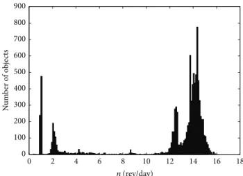
he present distribution of objects indicates the commen-surability between the frequencies of the mean motion�of object and the earth’s rotation motion. See the histogram in Figure 1.
InFigure 1, it is veriied that most of the objects is in the region13 ≤ � (rev/day) ≤ 15.
To study the resonant objects using the TLE data, a criterium is established for the resonant period�res, by the
condition�res > 300days. Note that the resonant period is
related to a resonant angle which can inluence the orbital motion of a particular artiicial satellite. he value of �res
helps to understand the inluence of each resonant angle, and this knowledge can provide a more rigorous analytical formulation of the problem. A minimum value is established for the resonant period in order to deine the main resonant angles that compose an orbital motion. he resonant angles are represented by the symbol�����.�resis obtained by the
relation
�res= 2�̇�
����, (1)
and ����̇� is calculated from [10]as follows:
�����(�, �, Ω, Θ)
= (� − 2� + �) � + (� − 2�) �
+ � (Ω − Θ − ���) + (� − �) �2,
(2)
where�,�,�,Ω,�, and�are the classical Keplerian elements:
�is the semimajor axis,�is the eccentricity,�is the inclination of the orbit plane with the equator,Ωis the longitude of the ascending node, �is the argument of pericentre and �is the mean anomaly, respectively;Θis the Greenwich sidereal time and���is the corresponding reference longitude along the equator. he term (� − �)(�/2) in (2) is a correction factor used in some representations of the earth gravitational potential [23–26]. his term is constant and do not appear
0 100 200 300 400 500 600 700 800 900
0 2 4 6 8 10 12 14 16 18
N
um
b
er o
f ob
jec
ts
n(rev/day)
Figure 1: Histogram of the mean motion of the cataloged objects.
in������/��used in the calculations of the present work. So,
̇�
����is deined as
̇�
����= (� − 2� + �) ̇� + (� − 2�) ̇� + � ( ̇Ω − ̇Θ) . (3)
Substituting� = � − 2�in (3), ���̇� is obtained as follows:
̇�
���= (� + �) ̇� + � ̇� + � ( ̇Ω − ̇Θ) . (4)
he terms ̇�, ̇Ω, and�̇ can be written considering the secular efect of the zonal harmonic�2as [7,27]
̇� = −34�2��(���
�)
2(1 − 5cos2(�))
(1 − �2)2 ,
̇Ω = −32�2��(���
�)
2 cos(�)
(1 − �2)2,
̇
� = ��− 34�2��(���
�)
2(1 − 3cos2(�))
(1 − �2)3/2 .
(5)
��is the earth mean equatorial radius and��= 6378.140 km,
�2is the second zonal harmonic,�2= 1.0826 × 10⁻³. he term ̇Θ, in rad/day, is
̇Θ ≈ 1.00273790926 × 2�. (6)
In order to use orbital elements compatible with the way in which two-line elements were generated, some corrections are done in the mean motion of the TLE data. Considering
�1as the mean motion of the 2-line, the semimajor axis�1is calculated [7]
�1= (√��
1) 2/3
, (7)
where�is the earth gravitational parameter,�= 3.986009 ×
1014m3/s2. Using�
1, (7), the parameter�1is calculated by (8) [7]
�1= 34�2�
2 �
�2
1
(3cos2(�) − 1)
Table 1: 2-line data of objects orbiting the earth.
File Number of data Number of objects
������� 2011 045 15360 9745
Now, a new semimajor axis��, used in the calculations of the resonant period, is deined using�1from (8) [7]
��= �1[1 − 13�1− �12− 13481 �13] , (9)
and the new mean motion ��, used in the calculations, is found considering the semimajor axis corrected��
��= √��3
�. (10)
Now, (1) to (10) can be used in a Fortran program to correct the observational data and to provide resonant angles and resonant periods related to orbital motions. he ile analyzed is “������� 2011 045” from the website Space Track [6], and it corresponds to February, 2011. In Table 1, the number of data and the number of objects are speciied.
he simulation identiied objects with resonant period greater than 300 days. Several values of the coeicients,�,
�, and�are considered in (2) producing diferent resonant angles to be analyzed by (1). SeeTable 2showing details about the results of the simulation.
Note that Table 2 shows only the data satisfying the established criterium,�res > 300days. he results show the
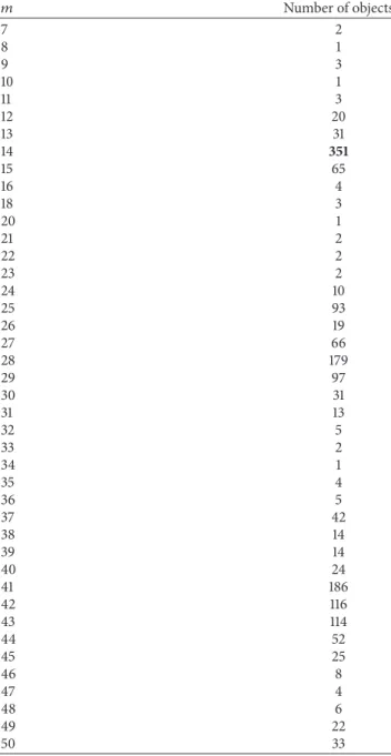
resonant angles and resonant periods which compose the orbital motions of the resonant objects.Table 3shows values of the coeicient�and the correspondent number of objects. It is possible to verify that most of the orbital motions are related to the coeicient� = 14considering the value of the semimajor axis up to15000km.
Comparing the number of objects satisfying the condi-tion of�res> 300days in the diferent regions,� < 15000km
and � ≥ 15000km, it is veriied that about 62.37% of the
resonant objects has� < 15000km. See this information in Table 4.
hese studies allow to investigate the real inluence of the resonance efect in the orbital dynamics of artiicial satellites and space debris. he number of resonant objects in comparison with the total number of objects in the TLE data shows the great inluence of the commensurability between the mean motion of the object and the earth’s rotation angular velocity in its orbits. In this way, a more detailed study about the resonant period and the resonant angles is necessary.
In the next section, the orbital motions of some space debris in resonance are studied.
3. Study of Objects in 14:1 Resonance
Considering the results of the simulations shown in the second section, some cataloged space debris is studied with respect to the time behavior of the semi-major axis, eccen-tricity, inclination, resonant period, resonant angle, and the
0
S
emima
jo
r axis (km)
Resonant period (days)
9
8
7
6
5
4
3
2
1
0 1 2 3 4 5 6 7 8 9 10
×104
×104
a ≥ 40000km
15000km≤ a < 40000km
a < 15000km
1:1resonance
2:1resonance
14:1resonance Object325
Object546
Object2986
Object4855
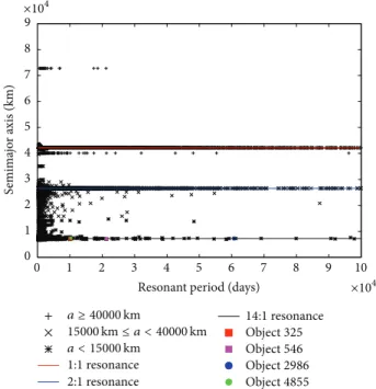
Figure 2: Semimajor axis versus resonant period of objects satisfy-ing the condition�res> 300days. he objects studied in LEO region are identiied by the numbers 325, 546, 2986, and 4855.
frequency analysis of the orbital elements. hese data are analyzed in this section observing the possible regular or irregular orbital motions.
Figure 2shows the semimajor axis versus resonant period
of objects satisfying the condition �res > 300 days. he
objects are distributed by the value of semimajor axis in three diferent regions: (1)� < 15000km, (2)15000km≤ � <
40000km, and (3) � ≥ 40000km.
Figure 2 shows some objects around the 1:1, 2:1 and
14:1 resonances. he orbital motions of these objects are inluenced by the resonance for several years and possible irregular motions can be conined in a region delimited for resonant angles with biggest resonant periods. In order to study the orbital motions of these objects, four cataloged space debris are analyzed in the LEO region; see Figure 2. From the TLE data, objects are identiied by the numbers 325, 546, 2986, and 4855. hese objects have been chosen because they show resonant period�res> 10000days.
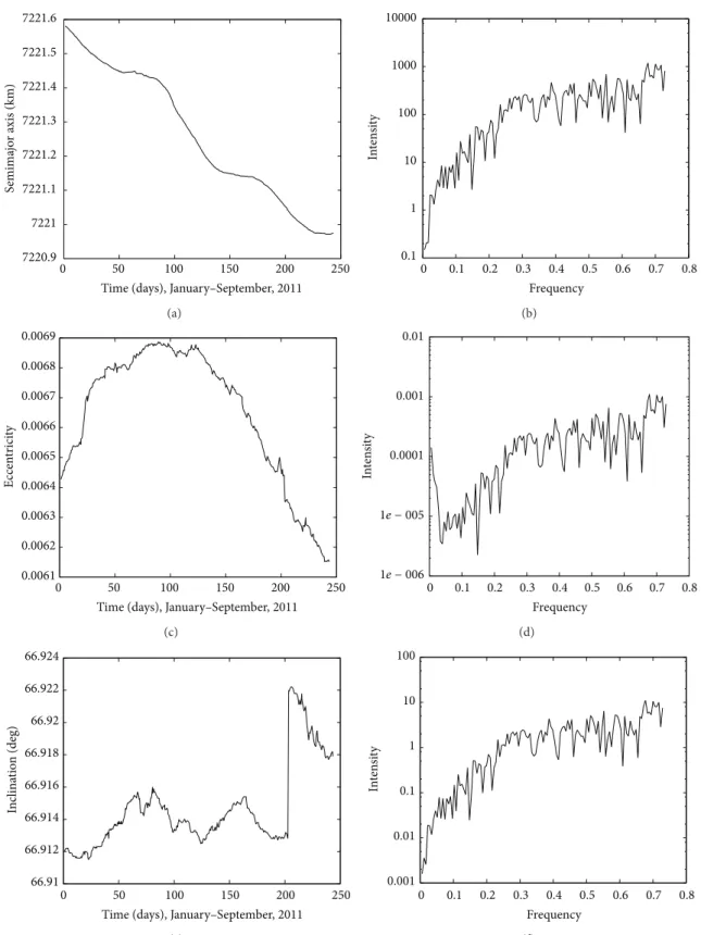
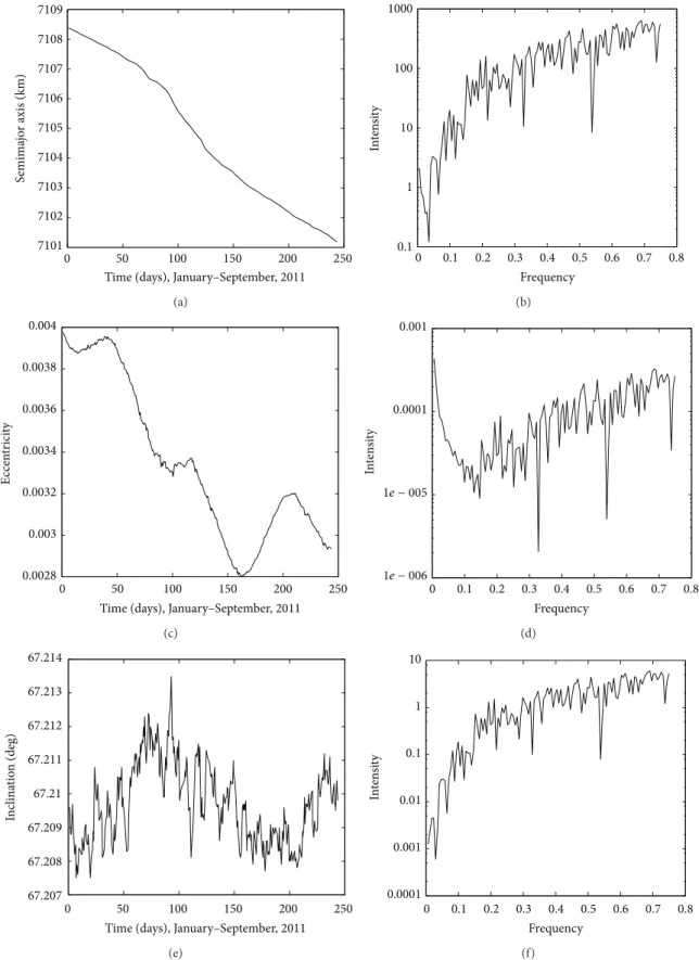
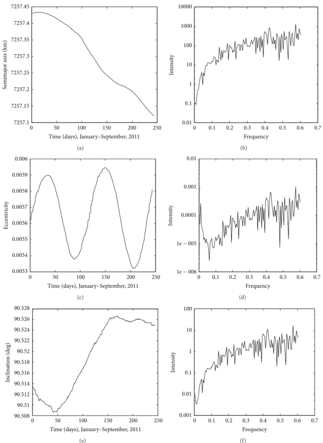
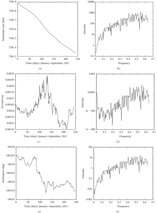
Figures 3, 4, 5, and 6 show the time behavior of the semimajor axis, eccentricity, and inclination of the objects 325, 546, 2986, and 4855, and the frequency analysis of these orbital elements.
Usually, in the studies of the dynamical systems with the purpose to identify chaos, the frequency analysis is considered for a long time. But, in low earth orbits, a big number of cataloged objects have their motions inluenced by diferent resonant periods and unknown objects can collide with each other providing more unpredictability in their motions. In this case, the frequency analysis can be more appropriate for a short time.
7220.9 7221 7221.1 7221.2 7221.3 7221.4 7221.5 7221.6
0 50 100 150 200 250
S
emima
jo
r axis (km)
Time (days), January–September,2011
(a)
0.1 1 10 100 1000 10000
0 0.1 0.2 0.3 0.4 0.5 0.6 0.7 0.8
Int
en
sit
y
Frequency
(b)
0.0061 0.0062 0.0063 0.0064 0.0065 0.0066 0.0067 0.0068 0.0069
Eccen
tr
ici
ty
0 50 100 150 200 250
Time (days), January–September,2011
(c)
0.0001 0.001 0.01
Int
en
sit
y
0 0.1 0.2 0.3 0.4 0.5 0.6 0.7 0.8 Frequency
1e − 006
1e − 005
(d)
66.91 66.912 66.914 66.916 66.918 66.92 66.922 66.924
In
clina
tio
n (deg)
0 50 100 150 200 250
Time (days), January–September,2011
(e)
0.001 0.01 0.1 1 10 100
Int
en
sit
y
0 0.1 0.2 0.3 0.4 0.5 0.6 0.7 0.8 Frequency
(f)
7101 7102 7103 7104 7105 7106 7107 7108 7109
0 50 100 150 200 250
S
emima
jo
r axis (km)
Time (days), January–September,2011
(a)
0.1 1 10 100 1000
Int
en
sit
y
0 0.1 0.2 0.3 0.4 0.5 0.6 0.7 0.8 Frequency
(b)
0.0028 0.003 0.0032 0.0034 0.0036 0.0038 0.004
Eccen
tr
ici
ty
0 50 100 150 200 250
Time (days), January–September,2011
(c)
0.0001 0.001
Int
en
sit
y
0 0.1 0.2 0.3 0.4 0.5 0.6 0.7 0.8 Frequency
1e − 006
1e − 005
(d)
67.207 67.208 67.209 67.21 67.211 67.212 67.213 67.214
In
clina
tio
n (deg)
0 50 100 150 200 250
Time (days), January–September,2011
(e)
0.0001 0.001 0.01 0.1 1 10
Int
en
sit
y
0 0.1 0.2 0.3 0.4 0.5 0.6 0.7 0.8 Frequency
(f)
7257.1 7257.15 7257.2 7257.25 7257.3 7257.35 7257.4 7257.45
S
emima
jo
r axis (km)
0 50 100 150 200 250
Time (days), January–September,2011
(a)
0.01 0.1 1 10 100 1000 10000
Int
en
sit
y
0 0.1 0.2 0.3 0.4 0.5 0.6 0.7 Frequency
(b)
0.0053 0.0054 0.0055 0.0056 0.0057 0.0058 0.0059 0.006
Eccen
tr
ici
ty
0 50 100 150 200 250
Time (days), January–September,2011
(c)
0.0001 0.001 0.01
Int
en
sit
y
0 0.1 0.2 0.3 0.4 0.5 0.6 0.7 Frequency
1e − 006
1e − 005
(d)
90.508 90.51 90.512 90.514 90.516 90.518 90.52 90.522 90.524 90.526 90.528
In
clina
tio
n (deg)
0 50 100 150 200 250
Time (days), January–September,2011
(e)
0.001 0.01 0.1 1 10 100
Int
en
sit
y
0 0.1 0.2 0.3 0.4 0.5 0.6 0.7 Frequency
(f)
7381.3 7381.4 7381.5 7381.6 7381.7 7381.8 7381.9
S
emima
jo
r axis (km)
0 50 100 150 200 250
Time (days), January–September,2011
(a)
0.1 1 10 100 1000 10000
Int
en
sit
y
0 0.1 0.2 0.3 0.4 0.5 0.6 0.7 Frequency
(b)
0.00145 0.0015 0.00155 0.0016 0.00165 0.0017 0.00175 0.0018 0.00185 0.0019
Eccen
tr
ici
ty
0 50 100 150 200 250
Time (days), January–September,2011
(c)
0.0001 0.001
Int
en
sit
y
0 0.1 0.2 0.3 0.4 0.5 0.6 0.7 Frequency
1e − 006
1e − 005
(d)
100.01 100.015 100.02 100.025 100.03 100.035 100.04
In
clina
tio
n (deg)
0 50 100 150 200 250
Time (days), January–September,2011
(e)
0.001 0.01 0.1 1 10 100
Int
en
sit
y
0 0.1 0.2 0.3 0.4 0.5 0.6 0.7 Frequency
(f)
Table 2: Results of the simulation: objects in resonant orbital motions.
Number of data Number of
diferent objects Coeicient� Coeicient� Coeicient�
3180 1276 −50 ≤ � ≤ 50 −5 ≤ � ≤ 5 1 ≤ � ≤ 50
Table 3: Number of objects according to the number of the coeicient�, considering the value of the semimajor axis up to 15000 km.
� Number of objects
7 2
8 1
9 3
10 1
11 3
12 20
13 31
14 351
15 65
16 4
18 3
20 1
21 2
22 2
23 2
24 10
25 93
26 19
27 66
28 179
29 97
30 31
31 13
32 5
33 2
34 1
35 4
36 5
37 42
38 14
39 14
40 24
41 186
42 116
43 114
44 52
45 25
46 8
47 4
48 6
49 22
50 33
dynamical systems. A brief description of the frequency analysis involving the Fast Fourier Transforms (FFT) is presented in what follows. See this method with more details in [28,29,33].
Generally, the frequency analysis is applied in the output of the numerical integration in the study of dynamical systems. However, in the present work, this analysis is used
Table 4: Number and percentage of objects satisfying the condition
�res> 300days.
� < 15000km 15000km≤ � <
40000km � ≥ 40000km
1276 331 439
62.37% 16.18% 21.46%
in the real data of the orbital motions of the objects 325, 546, 2986, and 4855, from the TLE data of the NORAD [6].
For regular motions, the orbital elements oe(�) show a dependence on time as follows [28,29,33]:
oe(�) = ∑
ℎ�ℎ� 2��hf�,
(11)
where�ℎrepresent the amplitudes,h ∈ Z�andf is a
fre-quency vector. he components offcompose the
fundamen-tal frequencies of motion, and the spectral decomposition of the orbital motion is obtained from the Fourier transform when the independent frequencies are constant in the course of time [33]. It is possible to observe thatfdepends on the
kind of trajectory [28].
he same numerical procedure is done for irregular and regular motions. he diference in behavior of these orbital motions is used to identify the two kinds of trajectories. he power spectrum of regular motion can be distinguished because it generally has a small number of frequency com-ponents produced by the Fourier transform. he irregular trajectories are not conditionally periodic and they do not compose an invariant tori. In this way, the Fourier transform of an orbital element, for example, is not a sum over Dirac
�-functions, and consequently the power spectrum is not discrete for irregular motions [28,33].
Observing the time behavior of the orbital elements of the objects 325, 546, 2986, and 4855 in Figures3,4,5, and6, one can verify possible regular and irregular motions in the trajectories of these space debris. he time behavior of the inclination shows irregularities. Analyzing object 325, note that, in 200 days, a fast increase in the inclination occurs, but, this variation is about0.01∘and it may be related to some disturbance added to the motion.
he power spectrum of the orbital elements is not discrete and they have a big number of frequency components in Figures3to6. So, it is also important to observe if the orbital motion is inluenced by diferent resonant angles.
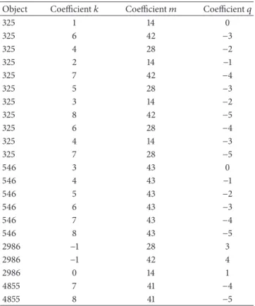
Table 5shows the resonant angles related to the orbital
0 20000 40000 60000 80000 100000
0 50 100 150 200 250
Res
o
na
n
t p
er
io
d (da
ys)
Time (days), January–September,2011
d𝜙2 14 −1/dt
d𝜙3 14 −2/dt
d𝜙4 14 −3/dt
d𝜙4 28 −2/dt
d𝜙5 28 −3/dt
d𝜙6 28 −4/dt
d𝜙7 28 −5/dt
d𝜙6 42 −3/dt
d𝜙7 42 −4/dt
d𝜙8 42 −5/dt
d𝜙1 14 0/dt
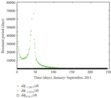
Figure 7: Time behavior of the resonant period corresponding to the orbital motion of object 325.
10000 20000 30000 40000 50000 60000 70000 80000
0 10 20 30 40 50 60 70
Res
o
na
n
t p
er
io
d
(da
ys)
Time (days), January–September,2011
d𝜙4 43 −1/dt
d𝜙5 43 −2/dt
d𝜙6 43 −3/dt
d𝜙7 43 −4/dt
d𝜙8 43 −5/dt
d𝜙3 43 0/dt
Figure 8: Time behavior of the resonant period corresponding to the orbital motion of object 546.
325 and 546, several resonant angles inluence their orbits simultaneously.
If the commensurability between the orbital motions of the object and the earth is deined by the parameter� and by the condition� = (� + �)/�, one can say that the exact 14:1 resonance is deined by the condition� = 1/14. his way, by analyzingTable 5, it is veriied that the motions of objects 325 and 2986 are inluenced by the exact 14:1 resonance,
� = 1/14, while the objects 546 and 4855 are inluenced by
resonant angles in the neighborhood of the exact resonance.
10000 20000 30000 40000 50000 60000 70000 80000
0 50 100 150 200 250
R
eso
n
an
t pe
ri
od
(
d
ay
s)
Time (days), January–September,2011
d𝜙0 14 1/dt
d𝜙−1 28 3/dt
d𝜙−1 42 4/dt
Figure 9: Time behavior of the resonant period corresponding to the orbital motion of object 2986.
10000 20000 30000 40000 50000 60000 70000 80000
0 50 100 150 200 250
Res
o
na
n
t p
er
io
d (da
ys)
Time (days), January–September,2011
d𝜙7 41 −4/dt
d𝜙8 41 −5/dt
Figure 10: Time behavior of the resonant period corresponding to the orbital motion of object 4855.
he condition�for object 546 is� = 3/43and for object 4855
is� = 3/41.
Figures 7, 8, 9, and 10 show the time behavior of the resonant period corresponding to the resonant angles presented inTable 5.
Analyzing the time behavior of the resonant period in Figures7,8,9, and10, it is veriied that the resonant angles remain conined for a few days. he term conined means that the orbital motion is inside a region delimited for resonant angles with biggest resonant periods. he orbital motion of object 546 has resonant angles which satisfy the established criterium�res > 300days for 70 days and, consequently, the
0 0.005 0.01 0.015 0.02 0.025
0 50 100 150 200 250 300 350 Time (days), January–September,2011
−0.005
−0.01
−0.015
−0.02
−0.025
d𝜙
kmq
/d
t
(rad/da
y)
d𝜙6 42 −3/dt
d𝜙4 28 −2/dt
d𝜙2 14 −1/dt
d𝜙7 42 −4/dt
d𝜙5 28 −3/dt
d𝜙3 14 −2/dt
d𝜙4 14 −3/dt
d𝜙8 42 −5/dt
d𝜙6 28 −4/dt
d𝜙7 28 −5/dt
d𝜙1 14 0/dt
Figure 11: Time behavior of ̇���� corresponding to the orbital motion of object 325.
0
0 20 40 60 80 100
Time (days), January–September,2011
0.005 0.01 0.015 0.02 0.025
−0.005
−0.01
−0.015 −0.02 −0.025
d𝜙
kmq
/d
t
(rad/da
y)
d𝜙4 43 −1/dt
d𝜙5 43 −2/dt
d𝜙6 43 −3/dt
d𝜙7 43 −4/dt
d𝜙8 43 −5/dt
d𝜙3 43 0/dt
Figure 12: Time behavior of ���̇� corresponding to the orbital motion of object 546.
objects 2986 and 4855, show a tendency to not remain in resonance, because the resonant period decreases from values greater than 10000 days to values smaller than 500 days. he orbital motion of object 325 is more inluenced by the 14:1 resonance and this fact can be observed by the time behavior of ���̇� ,Figure 11.
To continue the analysis about the irregular orbital motions, the time behavior of the ���̇� is studied verifying if diferent resonant angles describe the orbital dynamics of these objects at the same moment. his fact can indicate
0 0.01 0.02 0.03
0 50 100 150 200 250
Time (days), January–September,2011
−0.01
−0.02
d𝜙
kmq
/d
t
(rad/da
y)
d𝜙0 14 1/dt
d𝜙−1 28 3/dt
d𝜙−1 42 4/dt
Figure 13: Time behavior of ̇���� corresponding to the orbital motion of object 2986.
0 50 100 150 200 250 300
0 0.005 0.01 0.015 0.02 0.025
−0.005
−0.01
−0.015
−0.02
−0.025
Time (days), January–September,2011
d𝜙
kmq
/d
t
(rad/da
y)
d𝜙7 41 −4/dt
d𝜙8 41 −5/dt
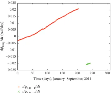
Figure 14: Time behavior of ̇���� corresponding to the orbital motion of object 4855.
irregular orbits requiring a full system with all resonant angles as described inTable 5. Figures11,12,13, and14show the time behavior of the ���̇� corresponding to the resonant angles presented inTable 5.
Analyzing the time behavior of the resonant angles ���̇� in Figures11,12,13, and14, it is possible to observe resonant angles in the exact 14:1 resonance:�1 14 0, �6 42 −3, �4 28 −2,
�2 14 −1,�7 42 −4,�5 28 −3,�3 14 −2,�8 42 −5,�6 28 −4,and�4 14 −3and
�7 28 −5 (object 325), �−1 28 3, and �−1 42 4 (object 2986) and resonant angles in the neighborhood of the 14:1 resonance:
Table 5: Resonant angles���� related to the orbital motions of objects 325, 546, 2986, and 4855.
Object Coeicient� Coeicient� Coeicient�
325 1 14 0
325 6 42 −3
325 4 28 −2
325 2 14 −1
325 7 42 −4
325 5 28 −3
325 3 14 −2
325 8 42 −5
325 6 28 −4
325 4 14 −3
325 7 28 −5
546 3 43 0
546 4 43 −1
546 5 43 −2
546 6 43 −3
546 7 43 −4
546 8 43 −5
2986 −1 28 3
2986 −1 42 4
2986 0 14 1
4855 7 41 −4
4855 8 41 −5
� = 1/14, � = 2/28, and � = 3/42. he time behavior
of curves with� = 2/28are similar and diferent of curves
with� = 3/42or� = 1/14. he orbital motion of object
546 is governed by distinct resonant angles, but, ater seventy days, the inluence of resonant efects decreases or disappears. Objects 325 and 2986 have their orbital motions inluenced by the exact 14:1 resonance and they need a full system with diferent resonant angles which compose their motions. Otherwise, the orbital motion of object 4855 is deined for resonant angles separately, which can be deined as a regular orbit.
he results and discussions show the complexity in the orbital dynamics of these objects caused by the resonance efects. Furthermore, the increasing number of space debris and collisions between them can cause big problems for artiicial satellites missions.
4. Conclusions
In this work, the orbital dynamics of synchronous space debris are studied. From the TLE data of the NORAD, objects orbiting the earth in resonant orbital motions are investigated.
Results show that some objects around the exact 1:1, 2:1, and 14:1 resonances remain in resonance for a long time. In other words, the orbital motions will be inluenced for resonant angles for several years and possible irregular motions can be conined in a region delimited for resonant angles with biggest resonant periods.
Analyzing the cataloged objects satisfying the established criterium of the resonant period greater than 300 days, four space debris (325, 546, 2986, and 4855) are studied observing the irregular characteristics in their orbits. he time behavior of the orbital elements and the respective frequency analysis are used to verify the orbits of these objects.
Several resonant angles inluence, simultaneously, the orbital motions of objects 325 and 2986. he time behavior of the inclination and the frequency analysis conirm the irregularities in their orbits. he orbital dynamics of object 546 is irstly inluenced by several resonant angles in the neighborhood of the 14:1 resonance, but, ater some days, the regular characteristic in its orbit seems to dominate. he time behavior of the ���̇� of object 4855 shows resonant angles separately indicating a regular orbit.
he resonant orbital dynamics of artiicial satellites and space debris can be described using observational data. Res-onant angles which compose the orbital motions are deined before the development of analytical model, providing more accuracy. Using the same procedure shown in the present work, the resonant periods associated with resonant angles can be determined and the study about any resonance, involving the commensurability between the mean motion of object and the earth’s rotation motion, can be described with more details.
Using real data, the time behavior of orbital elements allows to validate by comparison several analytical models describing perturbations in orbital motions, like atmospheric drag, solar radiation pressure, gravitational efects of the sun and the moon, for example. he frequency analysis from observational data is a new way to verify unstable regions.
In a future work, the method presented in this paper will be used to determine all resonant angles that inlu-ence a determined orbital motion and the analytical model presented in a previous paper [19]; it will be necessary to propagate the orbit, using each resonant angle and the correspondent resonant period previously determined. he description of the resonance problem is tending to a more understandable way.
Conflict of Interests
he authors declare that there is no conlict of interests regarding the publication of this paper.
Acknowledgments
his work was accomplished with support of the FAPESP under the Contracts nos. 2012/24369-0 and 2012/21023-6, SP, Brazil, CNPQ (Contract 303070/2011-0), and CAPES.
References
[3] Z. Changyin, Z. Wenxiang, H. Zengyao, and W. Hongbo, “Progress in space debris research,”Chinese Journal of Space Science, vol. 30, pp. 516–518, 2010.
[4] S. Nishida, S. Kawamoto, Y. Okawa, F. Terui, and S. Kitamura, “Space debris removal system using a small satellite,” Acta Astronautica, vol. 65, no. 1-2, pp. 95–102, 2009.
[5] M. J. Mechishnek, “Overview of the space debris environment,” Aerospace Report TR- 95(5231)-3, 1995.
[6] Space Track, “Archives of the 2-lines elements of NORAD,” 2011,
https://www.space-track.org/.
[7] F. R. Hoots and R. L. Roehrich, “Models for Propagation of NORAD Element Sets,” Spacetrack Report 3, 1980.
[8] H. K. Kuga, “Use of the ephemeris “2-lines” from NORAD in the orbital motion of the CBERS-1 satellite,” inProceedings of the 1st Congress of Dynamics, Control and Applications, no 1, pp. 925–930, 2002.
[9] V. Orlando, R. V. F. Lopes, and H. K. Kuga, “Flight dynamics team experience throughout four years of SCD1 in-orbit oper-ations: main issues, improvements and trends,” inProceedings of 12th International Symposium on Space Flight Dynamics, pp. 433–437, ESOC, Darmstadt, Germany, 1997.
[10] M. T. Lane, “An analytical treatment of resonance efects on satellite orbits,”Celestial Mechanics, vol. 42, no. 1–4, pp. 3–38, 1987.
[11] A. Jupp, “A solution of the ideal resonance problem for the case of libration,”Astronomical Journal, vol. 74, pp. 35–43, 1969. [12] T. A. Ely and K. C. Howell, “Long-term evolution of artiicial
satellite orbits due to resonant tesseral harmonics,”Journal of the Astronautical Sciences, vol. 44, no. 2, pp. 167–190, 1996. [13] D. M. Sanchez, T. Yokoyama, P. I. O. Brasil, and R. R. Cordeiro,
“Some initial conditions for disposed satellites of the systems GPS and Galileo constellations,” Mathematical Problems in Engineering, vol. 2009, Article ID 510759, 22 pages, 2009. [14] R. V. De Moraes and L. D. D. Ferreira, “GPS satellites orbits:
resonance,”Mathematical Problems in Engineering, vol. 2009, Article ID 347835, 12 pages, 2009.
[15] J. C. Sampaio, R. Vilhena de Moraes, and S. S. Fernandes, “Terrestrial artiicial satellites dynamics: resonant efects,” in Proceedings of the 21st International Congress of Mechanical Engineering, Natal, Brazil, 2011.
[16] J. C. Sampaio, R. Vilhena De Moraes, and S. Da Silva Fernan-des, “he orbital dynamics of synchronous satellites: irregular motions in the 2 : 1 resonance,” Mathematical Problems in Engineering, vol. 2012, Article ID 405870, 22 pages, 2012. [17] J. C. Sampaio, R. Vilhena de Moraes, and S. S. Fernandes,
“Arti-icial satellites dynamics: resonant efects,”Journal of Aerospace Engineering, Sciences and Applications, vol. 4, no. 2, pp. 1–14, 2012.
[18] J. C. Sampaio, E. Wnuk, R. Vilhena de Moraes, and S. S. Fernandes, “he orbital motion in the LEO region: objects in deep resonance,” inProceedings of the 39th COSPAR Scientific Assembly, Mysore, India, 2012.
[19] J. C. Sampaio, A. G. S. Neto, S. S. Fernandes, R. Vilhena de Moraes, and M. O. Terra, “Artiicial satellites orbits in 2 : 1 resonance: GPS constellation,”Acta Astronautica, vol. 81, no. 2, pp. 623–634, 2012.
[20] R. Vilhena de Moraes, J. C. Sampaio, S. da Silva Fernandes, and J. K. Formiga, “A semi-analytical approach to study resonances efects on the orbital motion of artiicial satellites,” in Proceed-ings of 23rd AAs- AIAA Space Flight Meeting, Kauai, Hawaii, USA, 2013.
[21] F. Delelie, A. Rossi, C. Portmann, G. M´etris, and F. Barlier, “Semi-analytical investigations of the long term evolution of the eccentricity of Galileo and GPS-like orbits,”Advances in Space Research, vol. 47, no. 5, pp. 811–821, 2011.
[22] L. Anselmo and C. Pardini, “Orbital evolution of the irst upper stages used for the new European and Chinese navigation satellite systems,”Acta Astronautica, vol. 68, no. 11-12, pp. 2066– 2079, 2011.
[23] J. P. Osorio,Disturbances of satellite orbits in the study of earth gravitational field, Portuguese Press, Porto, Portugal, 1973. [24] P. R. Grosso,Orbital motion of an artificial satellite in 2 : 1
reso-nance [M.S. thesis], ITA: Instituto Tecnol´ogico de Aeron´autica, S˜ao Paulo, Brazil, 1989.
[25] P. H. C. N. Lima Jr.,Resonant systems at high Eccentricities in the artificial satellites motion [Ph.D. thesis], ITA: Instituto Tecnol´ogico de Aeron´autica, S˜ao Paulo, Brazil, 1998.
[26] J. K. S. Formiga and R. Vilhena de Moraes, “Dynamical systems: an integrable kernel for resonance efects,”Journal of Computational Interdisciplinary Sciences, vol. 1, no. 2, pp. 89–94, 2009.
[27] J. Golebiwska, E. Wnuk, and I. Wytrzyszczak, “Space debris observation and evolution predictions, Sotware Algorithms Document (SAD),” ESA PECS Project 98088, Astronomical Observatory of the Adam Mickiewicz University, Poznan, Poland, 2010.
[28] G. E. Powell and I. C. Percival, “A spectral entropy method for distinguishing regular and irregular motion of Hamiltonian systems,”Journal of Physics A: General Physics, vol. 12, no. 11, pp. 2053–2071, 1979.
[29] J. Laskar, “Frequency analysis for multi-dimensional systems. Global dynamics and difusion,”Physica D: Nonlinear Phenom-ena, vol. 67, no. 1–3, pp. 257–281, 1993.
[30] M. Sidlichovsky and D. Nesvorny, “Frequency modiied fourier transform and its application to asteroids,”Celestial Mechanics and Dynamical Astronomy, vol. 65, no. 1-2, pp. 137–148, 1996. [31] N. Callegari Jr., T. A. Michtchenko, and S. Ferraz-Mello,
“Dynamics of two planets in the 2/1 mean-motion resonance,” Celestial Mechanics and Dynamical Astronomy, vol. 89, no. 3, pp. 201–234, 2004.
[32] N. Callegari Jr., S. Ferraz-Mello, and T. A. Michtchenko, “Dynamics of two planets in the 3/2 mean-motion resonance: application to the planetary system of the pulsar PSR B1257+12,” Celestial Mechanics and Dynamical Astronomy, vol. 94, no. 4, pp. 381–397, 2006.
Submit your manuscripts at
http://www.hindawi.com
Hindawi Publishing Corporation
http://www.hindawi.com Volume 2014
Mathematics
Journal ofHindawi Publishing Corporation
http://www.hindawi.com Volume 2014
Mathematical Problems in Engineering
Hindawi Publishing Corporation http://www.hindawi.com
Differential Equations International Journal of
Volume 2014 Hindawi Publishing Corporation
http://www.hindawi.com Volume 2014
Hindawi Publishing Corporation
http://www.hindawi.com Volume 2014
Hindawi Publishing Corporation
http://www.hindawi.com Volume 2014
Mathematical PhysicsAdvances in
Complex Analysis
Journal of Hindawi Publishing Corporationhttp://www.hindawi.com Volume 2014
Optimization
Journal ofHindawi Publishing Corporation
http://www.hindawi.com Volume 2014
Combinatorics
Hindawi Publishing Corporation
http://www.hindawi.com Volume 2014
International Journal of
Hindawi Publishing Corporation
http://www.hindawi.com Volume 2014
Journal of
Hindawi Publishing Corporation
http://www.hindawi.com Volume 2014
Function Spaces
Abstract and Applied Analysis Hindawi Publishing Corporation
http://www.hindawi.com Volume 2014
International Journal of Mathematics and Mathematical Sciences
Hindawi Publishing Corporation http://www.hindawi.com Volume 2014
The Scientiic
World Journal
Hindawi Publishing Corporation
http://www.hindawi.com Volume 2014
Hindawi Publishing Corporation
http://www.hindawi.com Volume 2014
Discrete Dynamics in Nature and Society
Hindawi Publishing Corporation
http://www.hindawi.com Volume 2014
Hindawi Publishing Corporation
http://www.hindawi.com Volume 2014
Discrete Mathematics
Journal ofHindawi Publishing Corporation
http://www.hindawi.com Volume 2014 Hindawi Publishing Corporation
http://www.hindawi.com Volume 2014