www.elsevier.com/locate/physa
Analysis of chaotic behaviour in the
population dynamics
Alcides Castro-e-Silva
a;∗, Americo T. Bernardes
baDepartamento de Fsica, Instituto de Ciˆencias Exatas, Universidade Federal de Minas Gerais, Caixa Postal 702, 30.123-970, Belo Horizonte=MG, Brazil
bDepartamento de Fsica, Universidade Federal de Ouro Preto, Campus do Morro de Cruzeiro, 35.400-000, Ouro Preto=MG, Brazil
Received 15 September 2000
Abstract
Recently, we have shown that the Penna bitstring model for population senescence can be used to model cyclic or chaotic behaviours in population dynamics. In this paper, we analyse the attractor of the dynamics, through the calculation of the Lyapunov exponents. We obtained that the dynamics is characterized by the existence of some small exponents, which we relate to the existence of homeochaos, needed for the generation of stability and diversity in living systems. c2001 Elsevier Science B.V. All rights reserved.
PACS:87.10.+e; 05.45.+b; 02.70.Lq
1. Introduction
Population dynamics can be viewed as the time evolution of one species, more than one, like the predator–prey case, or even the interactions among many species in a system. Dierent behaviours can be observed in the wild, and a sort of mathematical models are proposed to adjust to the experimental data. They vary from exponential growth (usually in the early stages of populations dynamics, where the populations are not constrained by external forces) to chaotic processes [1– 4]. So, most of the studies of population dynamics are done through mathematical models. The aim of such models (and computer simulations) is highlighted, if we take into account how dicult the observations in the wild are.
∗Corresponding author.
The rst model was introduced by Linnaeus in the XVI century: the exponential growth model. In this model, a given species can grow indenitely. Malthus, in 1798, pointed out that any population always has the constraints of food supply and envi-ronment carriage. Using an elephant as example, Darwin showed that after 750 years, there would be something like 9,000,000 elephants; descendants of one single couple. The elephant is a very slow breeding species. The Malthus theory has a deep inuence in Darwin’s idea of Natural Selection, where the environmental constraints would lead to the survival of the best tted [1]. Another model which takes advantage of this balance of growing and decline of a population is the Logistic Model. This model was introduced by Verhulst in 1844, and its discrete version, known as logistic map, was studied by Feigenbaum, who explored the universality in its period-doubling route to chaos. The relationship between population dynamics and the logistic map was intro-duced by May [5]. Such a map is very rich in terms of dynamical behaviours, and it is a mathematical example of period-doubling route to chaos, intermittent behaviour, tangent bifurcation and crises as well.
The ideas of heredity and mutation related to that of reproduction produced more sophisticated models (for a review, see Ref. [6]), very suitable for the methods of sta-tistical physics and computer simulations. One of those models is the Penna bitstring model [7,8] which has been introduced to simulate the dynamic of age-structured pop-ulations, with results in good agreement with observational data [9]. However, in most of the simulations, only one kind of dynamical behaviour was observed: a xed point, representing a stable population or the extinction, named Mutational Meltdown [10,11]. As we know, apart from the simple models discussed above, many others on population dynamics show chaotic dynamics [12–14] or non-trivial behaviour [15]. In our case, by properly tuning the parameters, we found limit cycles and nally a chaotic behaviour [16]. We investigated the return map and performed some tests like sensitivity to initial conditions, but the complete analysis of those data, via reconstruction of phase space, was missing. In the present work, by using the time series generated by the model, we reconstruct the attractor and evaluate the related Lyapunov exponents. So, our approach is dierent from that used by Miramontes and Ceccon [13], who used the analysis of correlation in order to characterize the chaotic state.
2. The model
environmental constraint, the Verhulst factor, that gives a probability of an individual for staying alive within the next time period, given by
Pl(t) = 1−N(t) Nmax
; (1)
whereNmax is the environmental carrying capacity (the maximum of individuals
sup-ported by the environment). No one can live more than 32 years. Sexual maturity is reached at the age of R, when the individual generates B ospring in this and the further years. The heredity appears as follows: the parent genome is copied to the ospring one, butM mutations are added randomly. Each mutation is introduced using the computer instruction OR, with a word mask that has just one bit = 1 at a ran-dom position, resulting always in a harmful mutation (0→1) or unmutated genome
(1→ 1), if that position already had a harmful mutation. Since the algorithm has a
random noise, the system is no longer deterministic. This is very important, because we are going to use the tools developed to analyse chaotic data in order to analyse the dynamic behaviour of our simulations. This problem will be discussed later.
The evolution of this system begins withN0 individuals. Along the simulation, many
individuals die due to environmental limitations and accumulation of genetic diseases. The survivors older than R will reproduce giving birth to B descendants each, and at this time, mutations will take place. Then, the total number, N(t), is reevaluated and the system goes on. The key for a chaotic behaviour is a correct balance be-tween a growing force, B, and an opposite force, the Verhulst factor. With the al-gorithm in mind, we can resume what we said above using a normalized logistic equation
X(t+ 1) =(t)X(t)[1−X(t)]; (2)
where X(t) =N(t)=Nmax and (t) is, roughly speaking, time and B dependent.
Dif-ferent from the logistic map, however, does not have a predened value. It does not have an explicit functional time dependence also, since it is obtained as the re-lationship between the population size at two times. As one knows, the dynamics of the logistic map is regulated by the growth rate. Some dynamic behaviours can also be obtained in the Penna model by properly switching the factor that regulates the population growth by increasing the birth rateB and xing the minimum age of repro-ductionR ¡ T, in order to assure that sexually immature will die only by the Verhulst factor.
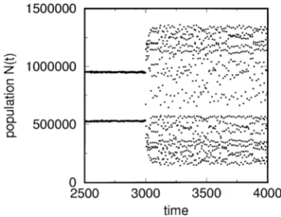
In our simulations, we have used the parameters: N0= 105 (106); Nmax= 1:5×
Fig. 1. Evolution of population showing two dierent regimes: a limit cycle with period 2 and a chaotic regime. The general parameters are:N0= 105; Nmax= 1:5×10⁶; M= 1; T= 6; R= 4; B= 20 for t ¡ to= 3000 and B= 35 fort¿to.
3. Attractor analysis
The technique used here is the reconstruction of the attractor based on time series introduced by Takens and Ma˜ne and known as embedding theorem [17,18]. The theorem says that for a scalar variable, x(t), which shows a multidimensional phase space, the geometric structure can be unfolded in a space made out of new vectors, namelyy(t) = [x(t); x(t+L); x(t+ 2L); : : : ; x(t+L(de−1))]. In this reconstruction, two
parameters are relevant: the time lag L and the embedding dimension de [19].
The time lag is important when we deal with continuous series or a set of dates with noise [21], and it is directly related to the creation of information. If the time lag is too large, any correlation betweenx(t) andx(t+L) is lost, because chaotic systems are intrinsically unstable. On the other hand, a very small L can destroy the independence
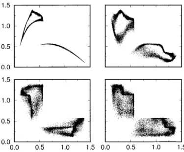
betweenx(t) andx(t+L). Roughly speaking, it means that we do not allow the system to produce new information about the state space. As one can observe in Fig. 2, there is a gradual loss of correlation betweenNt and the next point Nt+L as L increases. In
that gure, some plots ofNt versus Nt+L are shown for dierent values of L.
The choice of an embedding dimension is a little more critical in this kind of analysis. A correct value of de means that we are correctly projecting our dynamical
Fig. 2. Return map (Nt versus Nt+L) obtained in the chaotic regime for four values of time lag L. We show data plotted for four values ofL:L= 1 (top-left);L= 11 (top-right);L= 51 (bottom-left); andL= 101 (bottom-right). In the gure, we observe the gradual loss of correlation betweenNt and the next pointNt+L. Here,to= 5000 and we have 30,000 data points. The axes are in millions of individuals.
seem to be together are calledfalse nearest neighbour. In order to nd the embedding dimension, one has to remove those false nearest neighbours.
In our case, the time series is discrete, given by the total number of individuals at each year (or time step). It means that we have an Nt series instead of N(t), where
16t6tmax andtmax= 30;000. In order to simplify our notation, we start counting the
time when we changeB, i.e., our new variablet=t−to. So, the set of the data we deal
Fig. 3. Lyapunov exponents versus matrix dimensiondm (for details, see text). The left plot was obtained forL= 1 (de=dm): lled triangles represent the system withNmax= 1:5×10⁶while open circles represent a system 10 times bigger. The right plot shows data obtained by usingL= 5 (de= 5dm−4). The error bars are of the order of the symbol sizes.
attractor and the calculation of the embedding dimension in all cases. We also generated a series from a system 10 times bigger (N0= 106 and Nmax= 1:5×10⁷). In order to
assure that our results are not an artifact of the random number generator we used in our simulations (the usual linear congruential), we performed a set of simulations with the R250 [20]. We have not found signicant changes in the nal results.
The parameters which quantify the dynamics are the Lyapunov exponents, which describe how the orbits behave in the phase space. The algorithm [21] used here to evaluate the exponents assures only positive values. It means that the negative values of the exponents are indeed negative, but we do not know their magnitude. In this algorithm, the dependence of the embedding dimension on the time lag is given by the expression de= (dm−1)L+ 1, where dm is the dimension of the matrix used in
the calculation of the exponents. For this reason, we have useddm (matrix dimension)
instead of de (embedding dimension) in Fig. 3. This plot shows the Lyapunov
expo-nents versus the matrix dimension for two distinct cases. In the left plot, we show the values of the Lyapunov exponents obtained forL= 1, which means that dm andde are
equivalent. We compared the results for the two system sizes:Nmax= 1:5×10⁶ (lled
triangles), and for Nmax ten times bigger (open circles). First of all, we note that the
values obtained are independent of the system size, i.e., we observe the independence of the system dynamics with its size. However, as pointed out by Eckmann et al. [21], the persistent decreasing of the positive values of these exponents is a signal of the random noise existent in our system. In order to remove the eects of this random noise, we had to increase the time lag. The results obtained forL= 5 are shown in the right plot of Fig. 3. Now, de= 5dm−4. This result shows that some small positive
Lyapunov exponents arise.
hypotheses try to make a connection between experimental behaviours and the results obtained with mathematical or computational models, generally simple ones. In this way, all of them have a speculative characteristic. Two concepts have been pointed out as approaches to explain the evolution and dynamics of living systems: “the edge of chaos theory” and “homeochaos”. The idea behind the edge of chaos is that neither the linear regime nor the chaotic one would be a good place for living systems [23]. The intrinsic instability driven by chaos eliminates the recovering capability from tiny, introduced perturbations. A pure chaotic living system would not be able to main-tain its properties under constant changes caused by environmental constraints, like space, food, predators and so on. On the other hand, a stable regime is not a good solution as well, since the system would be frozen, incapable of evolving to new con-gurations, to respond to the evolutionary challenges and to be able to produce the tremendous diversity present in nature [24]. In the edge of chaos region, the system would take advantage of the complexity given by the chaotic region and the home-ostasis from the linear region. The edge of chaos requires that the system keeps itself trapped into a narrow dened region of the space of parameters, in order to avoid the chaotic and the linear regions, so the homeochaos term was coined to explain the diculty of a living system to self sustain in this kind of space. Stable states are tted only to stable environments, which is not the case of the problem studied here, where we have a competition of opposite forces: limited resources and high birth rate. The problem is that living systems are under strong non-linear interactions and any-way, can maintain some kind of stability and diversity. The idea is that homeochaos could do this in a better way than a xed point or chaos. The homeochaos shows three distinct features: (i) weak chaos, the positive Lyapunov exponents are close to zero; (ii) high-dimensional chaos, there are many positive Lyapunov exponents; and (iii) dynamic stability and robustness against external perturbations. The weak chaos is required in order to provide dynamical stability, and so, we have small oscillations when an external perturbation is introduced. In a strong chaos, large oscillations can pull the population down to a value close to zero, leading to extinction. Since home-ochaos is sustained in a region larger than the dynamics governed by a critical point (the chaos-linear frontier), it is more robust to a parameter change.
In conclusion, by calculating the Lyapunov exponents of the chaotic dynamic of a population given by the Penna model, we observed the fact that this system shows the basic features of homeochaos. This is the main feature which guarantees the existence of diversity and the fundamental stability which allows the survival of a population evolving under strong (and competing) natural pressures.
Acknowledgements
Fsica-UFMG. The simulations were performed in the Digital workstations at Physics Dept. of UFMG and UFOP. This work was partially supported by the Brazilian Agen-cies CNPq, FINEP and FAPEMIG.
References
[1] D. Brown, P. Rothery, Models in Biology: Mathematics Statistics and Computing, Wiley, New York, 1993.
[2] N.C. Stenseth, K.-S. Chan, E. Franstad, H. Tong, Proc. Roy. Soc. London B 265 (1998) 1957–1968. [3] B.E. Kendall et al., Ecology 265 (1999) 1789–1805.
[4] R.F. Costantino et al., Science 275 (1997) 389. [5] R. May, Science 186 (1974) 645.
[6] E. Baake, W. Gabriel, Annual Reviews of Computational Physics, Vol. VII, World Scientic, Singapore, 2000.
[7] T.J. Penna, J. Stat. Phys. 78 (1995) 1629.
[8] T.J. Penna, D. Stauer, Int. J. Mod. Phys. C 6 (1995) 233.
[9] S. Moss de Oliveira, P.M.C. de Oliveira, D. Stauer, Evolution, Money, War and Computers, Teubner, Stuttgart-Leipzig, 1999.
[10] M. Lynch, W. Gabriel, Evolution 44 (1990) 1725.
[11] A.T. Bernardes, Annual Reviews of Computational Physics, Vol. IV, World Scientic, Singapore, 1996, pp. 359 –395.
[12] V. Kirzhner, B.I. Lembrikov, A. Korol, E. Nevo, Physica A 249 (1998) 565–570. [13] O. Miramontes, E. Ceccon, Physica A 257 (1998) 439–447.
[14] M.G. Neubert, J. Theor. Biol. 189 (1997) 399–411. [15] M. Pascual, S.A. Levin, Ecology 80 (1999) 2225–2236.
[16] A.T. Bernardes, J.G. Moreira, A. Castro-e-Silva, Eur. Phys. J. B 1 (1998) 1–10.
[17] F. Takens, Dynamical Systems and Turbulence, Warwick 1980, Springer, Berlin, 1981, p. 366. [18] R. Ma˜ne, D. Rand, L.S. Young, Dynamical Systems and Turbulence, Warwick 1980, Springer, Berlin,
1981, p. 230.
[19] H.D.I. Abarbanel, Analysis of Observed Chaotic Data, Springer, New York, 1996. [20] S. Kirkpatrick, E.P. Stoll, J. Comput. Phys. 2 (1981) 517–526.
[21] J.-P. Eckmann, S. Olison Kamphorst, D. Ruelle, S. Ciliberto, Phys. Rev. A 34 (1986) 4971–4981. [22] K. Kaneko, Artif. Life 1 (1994) 163–177.