Geography and regional income convergence among Brazilian states

... #,FUNDAÇAo

... OETUUO VARGAS

,

EPGE

Escola de Pós-Graduaçlo em Economia

Seminário Especial

"Geography and Regional IncoDle

Convergence Alnong Brazilian States"

--,j

Prof. Naercio Menezes Filho (USP)

LOCAt.

Fundação Getulio Vargas

Praia de Botafogo, 190 - 10" andar - Auditório

UATA

20/07//99 (38 feira)

HORÁRIO

16:00h

•

,

Geography and Regional Income Convergence among Brazilian states

1

1. Introduction

Carlos Azzoni

Naércio Menezes Filho

Tatiane Menezes

Raul Silveira Neto

Department of Economics, Universidade de São Paulo, Brazil

In mainstream economics, the starting point for understanding the existence of poor

regions is the neoclassical exogenous growth model developed by Solow and Swan in

1956. According to this model, per capita income differentials among regions are

determi.ned by their respective initial endowments of resources, so that it is not so much

that there are poor regions, as given areas that have a greater concentration of poor

families. Such models are presented in greater detail in Barro and Sala-i Martin (1995).

Recent studies, such as Hall and Jones (1996), Chang (1994), Ravallion and Jalan (1996)

and Jalan and Ravaillon (1998b) have highlighted the importance of geographical,

institutional and political variables in determi.ning regional income differentials. According

to these authors, in certain circumstances the presence of poor families is determi.ned

endogenously, and not by the more widespread exogenous variables assumed in growth

I This is a preliminary paper on a research developed with support from the Interamerican Development

,

modeIs. Differing leveis of 'geographical capital', such as climate, local infrastructure,

access to public services and the knowledge about the local physical reality and adequate

technologies, would influence the use of private capital. That is, geographical variables

would affect the marginal return of private capital. The imperfect mobility of factors,

usua1ly assumed in this sort of mo deIs, would create the conditions for the persistency of

inequalities. The coexistence of increasing returns to geographical capital with

non-increasing returns to private capital is conceivable in this line of reasoning. Poor people

tend to live in poorly supplied regions. With the same personal characteristics, they

would be better of ifliving in a richer region.

This difference in diagnosis is reflected in the important issue ofpolicy recommendations. According to the first class of modeIs, regional inequality is to be solved by allowing free

mobility offactors, that should in turn result in long-term convergence of growth rates.

The second strand of the literature, on the other hand, can be used to justify regional

policies aiming at reducing regional inequality, such as public investments in

'geographical capital'.

The objective ofthis paper is to ofIer evidence on this controversy in the case ofstate

income inequalities in Brazil over the period 1981-1996. In section 2 some general

information on regional inequalities in Brazil is provided as well as a review of the some

existing empirical studies, creating the background for the study to be performed in the

paper. Section 3 presents a methodological discussion ofthe model to be estimated.

Section 4 presents the data used in the research and discusses the advantages and

limitations ofusing micro-data. Section 5 presents and discusses the econometric results,

which are commented on in the concluding section.

2. Regional inequalities in Brazil

Brazil is well known for its high leveis of regional income inequalities. In 1960, Brazil

had a GDP per capita ofUS$ 1,449. Thirty-five years later, in 1995, this figure had risen

to US$ 3,556, corresponding to an average growth of2.6% per year. Data on per capita

".

Brazilian states had figures above the national average, namely, São Paulo, Rio de Janeiro

and Rio Grande do Sul. The state of São Paulo was notable for a GDP per capita that

was almost 2 times the national average. The poorest state was Piauí, with a GDP per

capita that was 4.5 times less than the Brazilian average, and 8.9 times less than that of the state ofSão Paulo.1t is notable that nine ofthe ten poorest states in Brazil were in

the Northeast, and three ofthe four states ofthe Southeast were among the five richest

states in Brazil.

In 1995 a larger number of states were above the national average. Of these, the :first

two, São Paulo and Rio de Janeiro, are in the Southeast regiDo, whi1e the next three, Rio

Grande do Sul, Paraná and Santa Catarina, belong to the South region. The other

Southeastem states achieved visible improvements with regard to the national average

(e.g. the state ofMato Grosso). Ofthe tenpoorest states, eight are in the Northeast, and

two in the North regiDo, Amazonas and Pará, were notable for having declined in relative

terms since 1960, to stand among the ten states with the lowest GDP per capita. S~o

Paulo was still the richest state in 1995, with a GDP per capita that was 1.7 times the

national average, with an average growth rate of2.l% per year between 1960 and 1995,

0.5% below the national growth average. Piauí, on the other hand, was still the poorest

state in Brazil. It is nevertheless interesting to note, however, that whi1e in absolute terms

the state's position was considerably worse than the rest ofthe country, in relative terms it had improved, with a GDP per capita that was 3.7 times smaller than the national

average, and 6.1 times smaller than that ofthe richest state. Another interesting point is

that the state ofPiauí GDP per capita grew 3.1 % per year, one percentage point above

that ofthe state ofSão Paulo for the same period. These observations raise the question

as to whether or not there is an income convergence trend among Brazilian states.

Taking the neoclassical growth model as a basis, Ferreira and Diniz (1995), Schwartsman

(1996) and Zini (1998), analyzing the period initiated in 1970, could not reject the

hypothesis of absolute convergence. They estimated speeds of convergence among

Brazilian states that were above the leveIs predicted by the model. Azzoni (1999),

working with a longer series (1939-1996) also found indications ofabsolute convergence

..

•

spatial extemalities that conditions regional growth. That is to say, geographical

characteristics such as climate, public and private infrastructure (which could be

understood as reflecting 'geographical capital') may be affecting the growth rates of

states or regions, by in:tluencing the productivity of individual or family capital. This

would have decisive implications for public sector policies designed to combat poverty

and to improve incomes at regional and state leveI, since differences in living standards

would result not only from the initial conditions of families, as assumed by neoclassical

growth models, but also from differences in the 'geographical capital' between regions.

Since the previous models used for calculating convergence did not consider the effect of

geographical variables and these would tend to be positively correlated with initial

income, their results could be in fact reflecting conditional instead of absolute

convergence and could be under-estimating the true velocity to this convergence. We

thus propose to estimate the variation in household income per capita for Brazilian states

as a function of geographical, state and household variables, in order to capture not only

the in:tluence ofthe individual characteristics ofhouseholds on the convergence or

divergence of per capita income (along the tines of the neoclassical model), but also that

of spatial or geographical characteristics.

3. Theory

This section aims at presenting the neoclassic growth mo dei with exogenous savings,

geographic variables and fixed effects, as in Islam (1992), to be taken to the data.

Consider the production function, with labor augmenting technical progress:

Y(t)

=

Ka (t XA(t)L(t))'-a G

Where Y

=

product, K

=

capital, L

=

labour e G

=

geographic capital geographic (fixed in

"

L(t) = L(O)ent

A(t) = A(O)egt

where n and g are the (exogenously determined) population and technology rates of

growth. Capital accumulation per effective worker in the steady state will be given by:

A

dk (

)A

dt

=sy-

n+g+8 k,

h A

Y(t)

A

K(t)

w ere

y

=

A(t)L(t) '

k

=

A(t)L(t) ,

s

=

exogenous saving rate and õ

=

the

depreciation rate.

This equation implies steady state leveis of capital and product (per effective worker) described by:

I

k*

= ( s. G ) l-a

n+g+8 a

(

S ) l-a _ I

y*

=

n

+

g

+

8 . G l-a.

With the product per effective worker given by

y(t) =

fa(t)G,

we can approximate its time variation around the steady state to get (in logs):

d

ln~(t))

=

l[

ln(y

*)

-ln(y(t»)],

l =

(I -

a)(n

+

g

+

8).

We can now take the growth ofper capita product during the period 't = t2 -t1 by substituting the above value of

y

*:

ln(y(t2») -ln(y(tl») =

(1-

e-M)~ln(s)

- (l-e-M) - l

a (n

+

g

+ 8) +-1

1_(1_

e-M)ln(G)

l-a -a -a

-(1- e-M )ln(t1)

+

g(t2 - e--tT

tl)

+

(l_e--tT )ln(A(O»).

•

•

One can include human capital in the production function:

Where H is the stock ofhuman capital and ~ its coefficient (O<~<l). We now let Sk

and Sh be the fraction of income invested in physical and human capit~ respectively .

Thus, we will have the evolution ofthese capital per effective worker given by:

dk(t)

=

sky(t)- (n

+ g +

o)k(t)

dt

dh(t) =shy(t)-(n+g+o)h(t1

dt

In fact, we are assuming the same production function applies to human capit~ physical capital and consumption. Additiona1ly, by assuming (l+~<1, we preserve the decreasing marginal returns to capital and can study the steady state characteristics of the model.

From both equations above we can obtain the steady state leveis ofphysical and human capital:

I

" ( Sl-P sP G

J

l-a-p

k* = k h

n+g+o

Substituting into the production function we obtain the product of steady state:

_a ___ P_ a+p l-a-p l-a-PG1-a-p

". Sk Sh

Y = a+p

(n

+

g

+

O)l-a-p

We now approximate the income variation around the steady state to obtain:

where Â.

=

(l-(l-~)(n+g+õ).

,..

ln(y(t)) =

(1-

e-b )ln(V

)+

e-b ln(y(O))

Now we subtract the log of initial product per e:ffective worker and substitute for stead state leveI of product:

ln(y(t))-ln(y(O)) = (l-e-b ) a · ln(sk)+(I-e-b ) fi ln(sh)-(I-eb ) a+fi ln(n+g+8)

l-a-fi l-a-fi l-a-fi

+

1 ln(G)-(I-e-b )ln(y(O))

l-a-fi

Ifwe take this equation in per capita terms and consider the time period t2 - tI, we get:

ln(y(t₂»-ln(y(t))=(1-e-M

) a ln(Sk)

+

(1-e-..tT) fi ln(Sh)

l-a-fi l-a-fi

-(1-e-M

) a

+

fi ln(n

+

g + 8) + 1 lnG -(1-e-..tT)ln(y(tl)

+

(l-e-..tT)ln(A(O)

l-a-fi l-a-fi

+ g(t₂ _t)e..tT)

where t = t2 -tI.

4. Econometric Methodology

This section aims at representing the last equation in an form that is estimable with the data in hands. As the main aim ofthis version ofthis research is to investigate the roles of geographic and human capital variables on growth, we propose:

,

'I,

Yit-I = lny(t11

/!,.Y/t = lny(t2)-lny(t1)

r

= (l_e-lT

)

Si = (l-e-lT

) 1 [alns_k -(a+p)ln(n+g+c5)+lnA(O)/ 1 ]

1-a-p 1-a-p

171 = g&2-e-lT

tl)

where G and H are human capital and geographic variables.

4.1 The Construction of Cohorts

The data we use come from repeated cross-sections ofvery rich household surveys,

carried out by the Brazilian Census Bureau (see below). The use ofrnicro data to

examine issues of convergence has not, as far as we know, been done in the literature before. It is well known in the consumption and labor supply literature (see Browning et

al1985, Attanasio and Browning, 1994) that with repeated cross-sections it is possible to

construct demographic cohorts, based on date ofbirth calculate cohort-year means for alI

variables of interest, including income, education, labor force participation and living

conditions. We propose to extend this methodology to include the State ofresidence as

another grouping variable and derive state-cohort-year means for the variables of interest.

For example:

ncsy

LlnYi

- i

Y csy = - C . -_ _

ncsy

(11)

where: ncsy is the proportion ofhousehold heads bom in an interval of determined years

(e.g. 1940 to 1945) and living in state S in period t. (we contructed 10 birth cohorts).

We use the same procedure for alI other variables incldued in the analysis.

The advantages ofsuch a procedure are many-fold. First1y and most important1y, the use

ofrnicro-data alIows us to control for changes in the composition ofthe population in

Secondly, we can control for life-cycle and generation effects, which means that we are in

effect, considering the effect of geographic variables on income growth and convergence

within a generation or for a population with the same age. Thirdly, one can identify state

fixed effects without having to rely only on the time component of the series, since we

have got various (lO in our case) observations for a given state in a given year. Finally,

one can rely on differences across generations within a state-year group to identify the

effects ofhuman capital on growth, for example, that are not readly identified using

aggregate data (IsIam, 1994). The main disadvantage of using cohort levei data is that is there are measurement errors at the household leveI they are likely to be carried out to

the cohort means, unless the cell sizes are big.

In effect, we will be estimating an equation of the form:

L\Yict = JYict-l

+

Si

+

P1Hict

+

P2Gict

+

P3 XCit

+

P4 LFcit

+

Tlt

+

Gil

Where the subscript c means that the variables are now cohort-state-year means, X =

houdehold controls and LF = life cycle variables.

4. Data and data sources

The implementation of the model described above requires panel data, not easily available

in general. In the case ofBrazil we have repeated cross-sections ofa yearly household

survey (PNAD - Pesquisa Nacional por Amostra de Domicílios) conducted by IBGE, the

Brazilian Census Bureau, that can be used as a pseudo-panel, by constructing a model

that looks like an individual-levei model but is for cohorts (see Ravallion,1998). Due to

data limitations, only 19 out of27 states were considered in the study; the excluded states

•

Descriptive Statistics

The main variables in the ana1ysis are as disposed in Table 5. The dependent varialbe used

throughout is per capita monthly labor income from the main job. We have also used two

other variables, hourly labor income and total income with no apparent change in the

results.

The human capital variables we use are education ofthe head, education ofthe partner

and a measure of children delay in education. The geographic variables include access to

public sewage, water, light and garbage systems, urban and metropolitan areas, infant

mortality and life expectancy (as health indicators) and some climate variables. The life

cycle variables inc1ude age and participation ofhead, partner and children. ControIs

variables inc1ude the sex ofhead and measures ofhousehold wealth such as household

density and whether the household has a stove and fridge. We also inc1ude time and

cohort dummies. The correlations among the main variables used in the analysis is

presented in Table 1. The results are quite intuitive, indicating the income leveI is

positiveIy correlated with alI human capital, geographic, wealth and participation

indicators. The same results is basicalIy maintained with respect to income growth

Figures 3 to 36 in the appendix present an exhaustive description ofthe data, in order to

describe the main features ofthem, as well as examine the consistency ofthe information

on the mains variables used in the analysis between surveys.

5. Econometric results

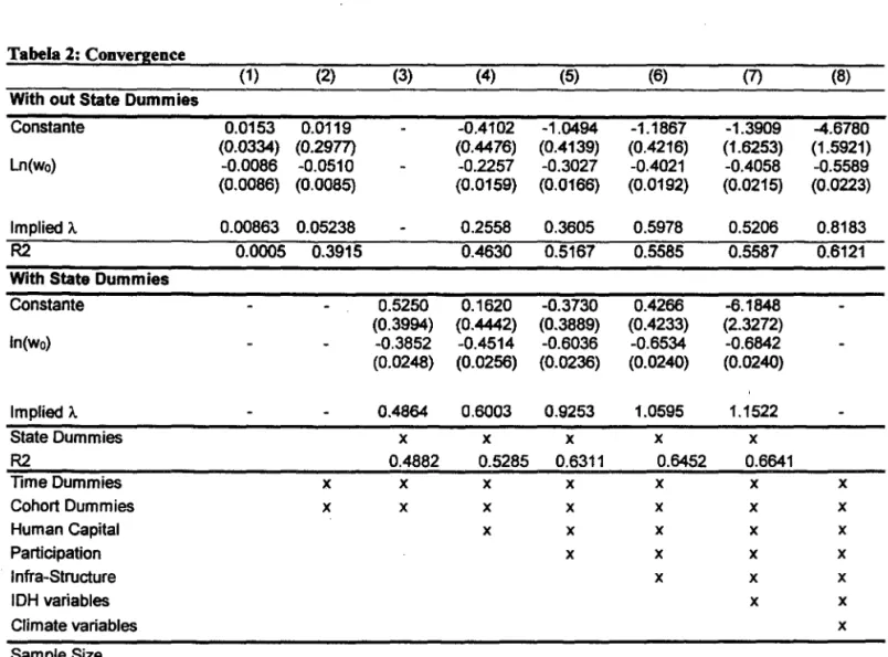
We now present the main results of estimating equation ( ). In table 2 the coefficients of

the lagged dependent variable are presented together with the implied  and the

estimated ve10city to half convergence. The upper part ofthe table refers to the results

without the state dummies as opposed to the bottom half. In column (1) there are no

other variables apart form the lagged dependent variable. This does not tak:e account of

•

significantly di:fferent from zero, which basically implies persistence in income di:fferences among states. Column (2) then includes the time and cohort dummies. The results are quite striking. Once we allow for di:fferences in birth cohorts, the coefficient on the lagged dependent variable is significant and quite big, which means that once one controIs for the di:fferent periods in the life cycle, there is absolute converge in income among Brazilian states.

In column (3) (QQttom part ofthe table) we include the state dummies, to control for di:fferences in technology, saving rates, population growth, preferences as well as

institutional among states. The results indicate that once you control for di:fferences in the steady-state growth rate among states, convergence (conditional convergence) actua11y tak:es place at a fast rate. Columns (4) to (8) in the upper part ofthe table shows that this is true even without controlling for the state fixed effects, but using human capital, participation or geographic variables instead. Columns (4) to (8) in the bottom part of the table show that once you control for state dummies, the marginal effect ofthe other variables on the speed of convergence is quite small.

In Table 3 the results ofthe state dummies are reported. The aim ofreporting this

coefficients is to examine the to what extent the states di:ffer in unobserved characteristics that are constant over time, such as technology, preferences, institutions, etc.,.

Furthermore, we want to shed light on the effect the other group ofvariables may have on the fixed effects, that is, to what extent some of human capital and specially

geographic variables can "explain" part ofthe estimated specific effects.

The states are ordered according to the average income leveI. Column (1) confirms this by presenting the results of a regression of income growth on state, time and cohort dummies. Column(2) includes the human capital variables and we can notice that some of the di:fferences between the state dummies and the reference state (Espirito Santo)

as well. The results presented in column(7) show that the differences in the estimated

coefticients are now reverted. This means that differences in infant mortality rates are also behind the state e:ffects.

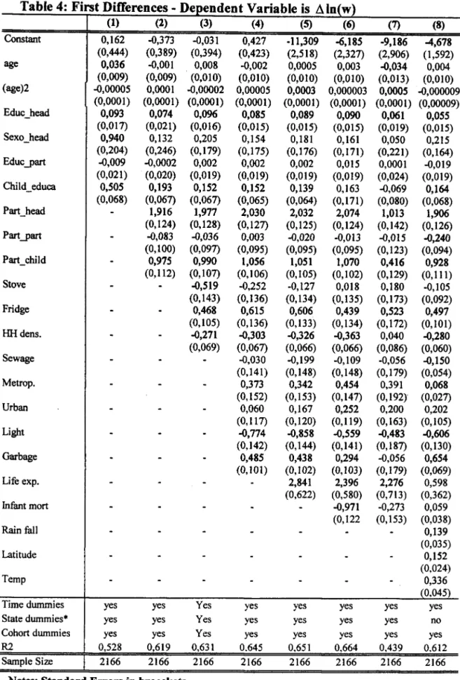
In Table 4, the coefticients (standard errors) ofthe human capital, life cycle, participation,

infra-structure, health and climate variables are set out. In the first column, one can note

that education ofthe head and of children are quite important in explaining income

growth. Moreover, the e:ffects oflabor market participation are quite important, and they

seem to be proxying for life-cycle e:ffects, as the age variables are now driven into

insignificancy. In column (4), the results indicate that percentage ofpopulation living in

metropolitan regions and access to garbage collection are positively correlated with

income growth. The results in column (5) and (6) are also very important as they

indicate that the quality ofhealth services is strongly correlated with growth, even

conditionally on state :6xed e:ffects and lagged income per capita. In column(7), the

lagged leveI is omitled from the regression, and it seems that household density,

metropolitan percentage and urban percentage are all positively correlated with the

omitled variables, as they now appear as insignificant.

6. Conclusions

The main objective ofthis paper is to shed some light on the e:ffects of geographic

variables on income per capita pattem of growth in different states in Brazil. To achieve

this aim, we proposed, for the first time in this strand ofthe economics literature, a

methodology to examine the issue of convergence using micro-data. We constructed

cohort/state/year averages of all variables of interest, and regressed income growth on a

variety ofhuman capital, life-cycle and geographic variables.

The main results indicate that geographic variables are important in explaining the

di:fference in income growth across the Brazilian States. This is shown by they joint

impact on the growth regressions and by the e:ffects that their inclusion has on the state

..

Brazil, once State E:ffects, human capital or geographic variables are controlled for. Moreover, there is some evidence that within cohort convergence takes place at a faster rate than across generations.

Altogether, the results indicate that human capital and geographic variables are important areas for governrnent intervention, as these are the mains factor behind the dMerences in steady-state rate of growth of income.

References

Attanasio, O and Browning, M. (1995) Consumption over the Life Cycle and the Business Cycle, American Economic Review, voI 85, pp. 1118-1136.

Azzoni, C. (1999). Economic Growth and Regional Income Inequalities in Brasil, Annals of Regional Science, forthcoming.

Barro, R e Sala-l-Martin, X. (1995), Economic Grow. McGraw-Hill, New York. --- (1997). TechnoIogical Diffusion, Convergence, and Growth, JEG, v. 2, pp. 1-26, Barro, R, Mankiw, G. e Sala-I-Martin, X., (1995). Capital Mobility in Neoclassical

Models ofGrowth, ERA, pp. 103-115, marcho

BIundell, R, Browning, M and Meghir, C (1994). Consumer Demand and the Life-Cycle Allocation ofHousehold Expenditures, Review of Economic Studies, voI. 61, pp. 57-80

Chang, R (1994), Income Inequality and Economic Growth: Evidence and Recent

Theories, Economic Review, July/ August, pp 1 - 9

Deaton, A. (1985) Panel Data from Time Series ofCross-Sections, Journal 01

Econometrics, vol. 30, pp 109-126

Ferreira A H and Diniz C C (1995) Convergencia entre las rentas per capita estaduales en Brasil. EURE-Revista Latioamericana de Estudios Urbano Regionales, Vol. XXI

No. 62, April

Hall,R and Jones, C. (1996). The Productive ofNations, National Bureau ofEconomic

Research, Working Paper Series, 5812

Helliwell, John, (1996), Do Borders Matter for Social Capital? Economic Growth and

Civic Culture in U.S. States and Canadian Provinces, National Bureau ofEconomic

Research, Working Paper Series 5863.

Jalan, J. and Ravallion, M (1 998a) Are there dynamic gains from a poor-area

development program? Journal 01 Public Economics, 67, pp. 65 - 85.

--- (1998b). Geographic Poverty Traps, Word Bank, May 15 pp 1- 31.

. Jones, Charles, (1995a) Times Series Tests ofEndogenous Growth Models, QJE, May.

495-525.

Jones, Charles, (1995b) R & D Based Models ofEconomic Growth, JPE, v.lOl, n. 4,

759-784.

Jones, Charles (1997) On the Evolution ofthe World Income Distribution, National

Bureau ofEconomic Research, Working Paper Series, 5812

Moffitt, R, (1993), Identification and Estimation ofDynamic Models with a Time Series

ofRepeated Cross-Sections, Journal 01 Econometrics, vol, 59, pp. 99-123

Ravallion, M. (1998), Poor areas, in Ullah, A and Giles D. (eds) Handbook 01 Applied

Economic Statistics.

Ravallion, M. (1998), Reaching Poor Areas in a Federal System, Policy Research Group

•

Ravallion, M. and Ialan, I. (1996), Growth Divergence Due Spatial Externalities,

Economic Letters 53,227-232.

Ravallion, M.and Wodon, Q. (1998), Poor Areas or

Iust

Poor People? Policy Research Working Paper 1798, World.Bank, Washington DC.

Romer, P. (1986); Increasing Returns and Long Run Growth; Journal of Political

Economy,v.94,pp.1002-37

Schwartsman, A.. Convergence Across Brazilian States, Discussion Paper, nO 02/96. IPE,

Universidade de São Paulo, 1996.

Zini A A Ir (1998) Regional income convergence in Brazil and its socio-economic

4. ..

.•

...

Table I - Correlations among variables

Ln(w) Dln(w) Educ_ Sex Part_ Educ_ Part_ Stove Fridge HH Metrop Urban Water Light Sewage Garbage Rainfàll Latit Temp. life Inlãnt head head head art ch dens ex t. morto Ln(w)

D In(w) 0.37S·

Educ_head 0.710' 0.134'

Sex_head 0.541' 0.178' 0.497'

Part.Jl8rt 0.208' 0.110' O.4IS· 0.321'

Educ.Jl8rt 0.664' 0.153' 0.946' 0.656' 0.517'

Part _ children -0.266' -0.095' -0.594' -0.677' -0.233' -0.710'

Stove 0.433' 0.033 0.476' -0.012 0.043' 0.385' 0.048'

Fridge 0.558' 0.036 0.65S· -0.051' 0.252' 0.495' 0.107' 0.666'

HHDensity 0.002 0.077' -O.lS7· 0.48S· 0.159' -0.011 -0.255' -0.492' -0.561'

Metrop 0.2%' 0.008 0.414' -007S' -0.013 0.255' -0.063' 0.316* 0.419' -0.174*

Urban 0.50S· 0.063' 0.652' -0.039' 0.039' 0.494' -0.072' 0.711' 0.773' -0.485' 0.605'

Water 0.554' 0.053" 0.617" -0.019 0.004 0.467" 0.031 0.698* 0.83S· -0.506" 0.448" 0.785*

Light 0.455' 0.039' 0.662' -0.074' 0.264' 0.531' -0.019 0.743' 0.8SI" -0.612' 0.376' 0.S05· 0.SI8·

Sewage 0.536' 0.029 0.605' -0.059' -0.03 0.429' 0.054' 0.690' 0.S21· -O.50S· 0.535' 0.S39· 0.853' 0.792'

Garbage 0.505' 0.03 0.609' -0.071' 0.093' 0.460' 0.011 0.672' O.SIS· -0.527' 0.447' 0.864' O.SOO· 0.S34· 0.S30·

Rainlãll 0.419' 0.002 0.314' 0.144' 0.050' 0.221" 0.086' 0.105' 0.490' -0.191' 0.073' 0.165' 0.327' 0.231' 0.364' 0.270'

Latitude 0.607' 0.033 0.54S· 0.067' -0.002 0.384' 0.063' 0.581' 0.7S8· -0.495' 0.377' 0.602' 0.749' 0.630' 0.704' 0.645' 0.645'

Temp -0.546' -0.033 -0.450' -0.099' -0.040' -0.333' -0.062' -0.547' -0.664' 0.451' -0.228' -0.498' -0.592' -0.535' -0.510' -0.541' -0.454' -O.S58·

life expec. 0.251' O 0.473' -0.157' 0.449' 0.362' 0.119' 0.419' 0.73S· -0.620' 0.158' 0.463' 0.4S5" 0.681' 0.505' 0.539' 0.429' 0.534' -0.522'

•

Tabela 2: Convergence

(1) (2) (3) (4) (5) (6) (7) (8)

With out State Dummies

Constante 0.0153 0.0119 -0.4102 -1.0494 -1.1867 -1.3909 -4.6780

(0.0334) (0.2977) (0.4476) (0.4139) (0.4216) (1.6253) (1.5921)

Ln(wo) -0.0086 -0.0510 -0.2257 -0.3027 -0.4021 -0.4058 -0.5589

(0.0086) (0.0085) (0.0159) (0.0166) (0.0192) (O.0215) (0.0223)

Implied À 0.00863 0.05238 0.2558 0.3605 0.5978 0.5206 0.8183

R2 0.0005 0.3915 0.4630 0.5167 0.5585 0.5587 0.6121

With State Dummies

Constante 0.5250 0.1620 -0.3730 0.4266 -6.1848

(0.3994) (0.4442) (0.3889) (0.4233) (2.3272)

In(wo) -0.3852 -0.4514 -0.6036 -0.6534 -0.6842

(0.0248) (0.0256) (0.0236) (0.0240) (0.0240)

Implied À 0.4864 0.6003 0.9253 1.0595 1.1522

State Oummies x x x x x

R2 0.4882 0.5285 0.6311 0.6452 0.6641

Time Oummies x x x x x x x

Cohort Oummies x x x x x x x

Human Capital x x x x x

Participation x x x x

Infra-Structure x x x

IOH variables x x

Climate variables x

T able 3 S

.

.

tate Dummies - Dependent Variable is AIn(\\'}

(1) (2) (3) (4) (5) (6) (7) (8)

São Paulo 0,277 0,233 .0,365 0,360 0,033 0,045 -0,068 -0,423 (0,030) (0,032) (0,030) (0,036) (0,085) (0,085) (0,083) (0,105) Mato Grosso do Sul 0,157 0,181 0,204 0,221 0,144 0,113 0,075 -0,107 (0,026) (0,026) (0,023) (0,036) (0,034) (0,036) (0,036) (0,043) Rio de Janeiro 0,146 0,071 0,185 0,182 -0,176 -0,114 -0,293 -0,479 (0,027) (0,034) (0,031) (0,034) (0,121) (0,122) (0,117) (0,153) Rio grande do Sul 0,136 0,118 0,156 0,118 -0,094 -0,200 -0,597 -0,471

(0,026) (0,028) (0,026) (0,027) (0,068) (0,074) (0,085) (0,107) Mato Grosso 0,130 0,194 0,191 0,257 0,157 0,196 0,333 0,017

(0,026) (0,028) (0,027) (0,029) (0,039) (0,038) (0,045) (0,053) Santa Catarina 0,145 0,085 0,147 0,084 0,063 -0,052 -0,161 -0,218

(0,033) (0,034) (0,030) (0,033) (0,044) (0,052) (0,053) (0,065) Paraná 0,120 0,134 0,129 0,141 -0,023 -0,053 0,001 -0,165

(0,024) (0,024) (0,023) (0,023) (0,050) (0,052) (0,052) (0,065) Goiás 0,072 O,IS8 0,170 0,215 0,170 0,177 0,141 0,003

(0,024) (0,027) (0,025) (0,025) (0,029) (0,029) (0,030) (0,034) Minas Gerais 0,050 0,109 0,127 0,165 0,040 0,055 0,060 -0,042

(0,020) (0,023) (0,022) (0,022) (0,041) (0,042) (0,041) (0,052) Sergipe -0,097 0,083 0,047 0,104 0,061 0,213 0,937 0,450

(0,028) (0,036) (0,032) (0,034) (0,042) (0,054) (0,115) (0,142) Bahia -0,123 0,048 -0,008 0,069 -0,039 0,046 0,653 0,252

(0,023) (0,030) (0,029) (0,038) (0,059) (0,060) (0,105) (0,131) Pernambuco -0,147 -0,018 -0,021 0,059 -O,llO 0,059 0,904 0,353

(0,023) (0,028) (0,027) (0,031) (0,075) (0,082) . (0,147) (0,180) Alagoas -0,148 0,025 0,049 0,098 0,074 0,347 1,507 0,733

(0,028) (0,035) (0,032) (0,038) (0,050) (0,074) (0,177) (0,219) Rio Grande do Norte -0,134 -0,033 -0,036 0,021 -0,017 0,157 1,110 0,603

(0,028) (0,033) (0,029) (0,035) (0,046) (0,057) (0,143) (0,178) Ceará -0,214 -0,055 -0,139 -0,030 -0,223 -0,100 0,823 0,373

(0,026) (0,034) (0,032) (0,039) (0,083) (0,084) (0,154) (0,192) Paraíba -0,281 -0,158 -0,228 -0,137 -0,193 0,017 1,012 0,661

(0,031) (0,036) (0,033) (0,039) (0,046) (0,064) (0,151) (0,189) Maranhão -0,289 -0,099 -0,262 -0,228 -0,172 -0,045 0,949 0,516

(0,038) (0,045) (0,043) (0,067) (0,076) (0,074) (0,152) (0,191) Piauí -0,450 -0,274 -0,462 -0,441 -0,485 -0,392 0,299 0,363

(0,041) (0,048) (0,046) (0,059) (0,074) (0,073) JO,1231 (0,148) Time Durnrnies x x x x x x x x

Cohort Durnmies x x x x x x x x

Hurnan Capital x x x x x x x Participation x x x x x x HH Characteristics x x x x x

Infra-Structure x x x x

Life Expectance x x x

Infant Mortality x x

Sample Size 2166 2166 2166 2166 2166 2166 2166 2166 R2 0,488 0,528 0,619 0,631 0,645 0,651 0,664 0,439

Notes: Standard Errors in bracckets.

lThe state ofEspírito Santo is taken as reference

•

Table 4: First DifTerences - Dependent Variable is Aln(w}

(1) (2) (3)

Constant 0,162 -0,373 -0,031

(0,444) (0,389) (0,394)

age 0,036 -0,001 0,008

(0,009) (0,009) (0,010)

(age)2 -0,00005 0,0001 -0,00002

(0,0001) (0,0001) (0,0001)

Educ_head 0,093 0,074 0,096

(0,017) (0,021) (0,016)

Sexo_head 0,940 0,132 0,205

(0,204) (0,246) (0,179)

EducJ>art -0,009 -0,0002 0,002

(0,021) (0,020) (0,019)

Child_educa 0,505 0,193 0,152

(0,068) (0,067) (0,067)

Part_head

-

1,916 1,977

(0,124) (0,128)

PartJ>art

-

-0,083 -0,036

(0,100) (0,097)

Part_child

-

0,975 0,990

(0,112) (0,107)

Stove

-

-

-0,519

(0,143)

Fridge

-

-

0,468

(0,105)

HHdens.

-

-

-0,271

(0,069)

Sewage

-

-

-Metrop.

-

-

-Urban

-

-

-Light

-

-

-Garbage

-

-

-Life exp.

-

-

-Infant mort

-

-

-Rain fali

-

-

-Latitude

-

-

-Temp

-

-

-Time dummies yes yes Yes

Statedummies· yes yes Yes

Cohort dummies yes yes Yes

R2 0,528 0,619 0,631

Sample Slze

I

2166 2166 2166

Notes: Standard Errors in bracckets.

I The state of Espírito Santo is taken as reference

1 AlI colluns except (7) incIude initiaI income.

(4) (5) (6)

0,427 -11,309 -6,185

(0,423) (2,518) (2,327)

-0,002 0,0005 0,003

(0,010) (0,010) (0,010)

0,00005 0,0003 0,000003

(0,0001) (0,0001) (0,0001)

0,085 0,089 0,090

(0,015) (0,015) (0,015)

0,154 0,181 0,161

(0,175) (0,176) (0,171)

0,002 0,002 0,015

(0,019) (0,019) (0,019)

0,152 0,139 0,163

(0,065) (0,064) (0,171)

2,030 2,032 2,074

(0,127) (0,125) (0,124)

0,003 -0,020 -0,013

(0,095) (0,095) (0,095)

1,056 1,051 1,070

(0,106) (0,105) (0,102)

-0,252 -0,127 0,018

(0,136) (0,134) (0,135)

0,615 0,606 0,439

(0,136) (0,133) (0,134)

-0,303 -0,326 -0,363

(0,067) (0,066) (0,066)

-0,030 -0,199 -0,109

(0,141) (0,148) (0,148)

0,373 0,342 0,454

(0,152) (0,153) (0,147)

0,060 0,167 0,252

(0,117) (0,120) (0,119)

-0,774 -0,858 -0,559

(0,142) (0,144) (0,141)

0,485 0,438 0,294

(0,101) (0,102) (0,103)

-

2,841 2,396

(0,622) (0,580)

-

-

-0,971

(0,122

-

-

--

-

--

-

-yes yes yes

yes yes yes

yes yes yes

0.645 0.651 0,664

2166 2166 2166

(7) (8)

-9,186 -4,678

(2,906) (1,592)

-0,034 0,004

(0,013) (0,010)

0,0005 -0,000009 (0,0001) (0,00009)

0,061 0,055

(0,019) (0,015)

0,050 0,215

(0,221) (0,164)

0,0001 -0,019

(0,024) (0,019)

-0,069 0,164

(0,080) (0,068)

1,013 1,906

(0,142) (0,126)

-0,015 -0,240

(0,123) (0,094)

0,416 0,928

(0,129) (0,111)

0,180 -0,105

(0,173) (0,092)

0,523 0,497

(0,172) (0,101)

0,040 -0,280

(0,086) (0,060)

-0,056 -0,150

(0,179) (0,054)

0,391 0,068

(0,192) (0,027)

0,200 0,202

(0,163) (0,105)

-0,483 -0,606

(0,187) (0,130)

-0,056 0,654

(0,179) (0,069)

2,276 0,598

(0,713) (0,362)

-0,273 0,059

(0,153) (0,038)

-

0,139 (0,035)

-

0,152 (0,024)

-

0,336 (0.045)

yes yes

yes no

yes yes

0,439 0,612

• T bl 5 V . bl d a e ana e escnptIon

Code Brazil

_J

NE and CO

_I

South and SE

Avg SO Avg SO Avg SO

DepeDdeDt Vlrilble:

monthly income in the main occupation ofhousehold head 71103 156911 56522 121330 96097 201583

Flmily:

gender ofthe household head (male = I; female = O) Sexo_head 0,835 0,079 0,832 0,077 0,840 0,081

Education: household head Educ_head 3,858 1,654 3,199 1,367 4,987 1,486

(years) spouse(orhusband) Educ .-JlIIrt 3,151 1,429 2,747 1,305 3,845 1,366

Particil1!!tion household head (previous week) Part_head 0,847 0,161 0,857 0,145 0,830 0,183

in labor furce spouse (or husband) Part.-PBrt 0,304 0,115 0,298 0,111 0,315 0,119

(yes=I; no=O) children (average, yes=l; no=O) Part_child 0,246 0,171 0,238 0,161 0,260 0,187

Housebold:

Density - occupants per room HHdens. 0,913 0,206 0,982 0,203 0,796 0,152

Proprietorship ofhouse (owned = I; not owned = O) 0,690 0,143 0,702 0,139 0,669 0,146

Availability of ~ (yes = I; no = O) Stove 0,915 0,1l0 0,876 0,121 0,983 0,016

Availability ofrefrigerator (yes= I; no = O) Fridge 0,572 0,208 0,457 0,147 ' 0,771 0,136

Electricity (supplied with electricity = I; not supplied = O) Light 0,769 0,166 0,694 0,152 0,898 0,092

Water (supplied by the public system = I; not supplied = O) Water 0,621 0,185 0,522 0,140 0,792 0,116

Sewage (served by the public system = I; not served = O) Sewage 0,484 0,170 0,387 0,108 0,650 0,122

~ (served by the public system = I; not served = O) Garbage 0,497 0,191 0,418 0,163 0,633 0,157

Geograpbical:

UrbanIrural (urban = I; rural = O) Metrop. 0,164 0,227 0,082 0,149 0,303 0,266

Metropolitan region (metropolitan = I; non-metropolitan=O) Urban 0,675 0,140 0,618 0,121 0,773 0,114

Lifeexp. 61,199 4,001 59,694 3,640 63,778 3,196

Infànt mort 65,473 35,407 82,187 34,048 36,821 10,758

Distance from the sea (from the state' s capitais) - km 226,252 203,941 267,627 240,303 155,323 77,182

Average temperature in the Winter - Celsius degrees Temp 19,892 4,334 21,778 3,738 16,661 3,241

A1titude-m 328,073 164,765 269,625 114,701 428,269 187,772

Longitude - degrees Latitude -13,315 7,094 -8,839 3,049 -20,987 5,240

..

,

...

Tabela 6a

Variable São Paulo Rio de Janeiro Minas Gerais Paraná Santa Catarina Rio Grande do Espírito santo Maranhão Piaui Ceará

Sul

--- Avg SD Avg SD Avg SD Avg SD Avg SD Avg SD Avg SD Avg SD Avg SD Avg

rendapc 120970 246894 117826 236551 70110 142470 84753 171656 94613 205678 108813 227253 75598 152146 34395 64530 32334 63218 43465

Sexo head 0,836 0,076 0,797 0,087 0,828 0,084 0,858 0,066 0,875 0,076 0,836 0,078 0,849 0,076 0,835 0,067 0,830 0,063 0,846

Educ head 5,551 1,255 6,292 1,050 4,239 1,246 4,363 1,466 4,860 1,445 5,213 1,322 4,393 1,385 2,340 1,039 2,329 1,155 2,744

Educ --'part 4,080 1,308 4,344 1,199 3,408 1,312 3,402 1,378 4,003 1,360 4,132 1,333 3,542 1,356 2,108 1,057 2,156 1,145 2,481

Part head 0,813 0,204 0,791 0,218 0,830 0,165 0,856 0,156 0,836 0,182 0,842 0,173 0,840 0,168 0,898 0,108 0,879 0,122 0,868

Part--.part 0,261 0,099 0,274 0,090 0,262 0,106 0,322 0,106 0,382 0,120 0,391 0,119 0,314 0,112 0,380 0,109 0,334 0,130 0,335

Part_child 0,259 0,190 0,210 0,160 0,255 0,185 0,293 0,193 0,295 0,204 0,244 0,168 0,267 0,193 0,252 0,155 0,248 0,165 0,232

HHdens. 0,834 0,153 0,785 0,127 0,796 0,136 0,861 0,168 0,744 0,153 0,741 0,146 0,810 0,138 1,193 0,195 1,092 O,229 1,062

Stove 0,988 O,Oll 0,984 0,010 0,983 0,011 0,978 0,017 0,976 0,026 0,986 0,010 0,985 0,017 0,634 0,125 0,697 0,147 0,906

Fridge 0,881 0,068 0,878 0,065 0,601 0,101 0,690 0,114 0,838 0,078 0,816 0,076 0,690 0,118 0,302 0,088 0,327 0,106 0,362

Light 0,963 0,075 0,973 0,019 0,806 0,101 0,853 0,096 0,928 0,039 0,899 0,053 0,865 0,089 0,507 0,135 0,484 0,124 0,601

Water 0,934 0,033 0,869 0,062 0,742 0,072 0,751 0,095 0,734 0,144 0,793 0,086 0,723 0,092 0,294 0,068 0,380 0,077 0,367

Sewage 0,851 0,041 0,750 0,044 0,681 0,046 0,572 0,032 0,506 0,061 0,549 0,052 0,638 0,048 0,246 0,040 0,200 0,041 0,300

Garbage 0,890 0,032 0,722 0,065 0,527 0,082 0,619 0,104 0,543 0,132 0,654 0,085 0,478 0,084 0,134 0,068 0,189 0,070 0,320

Metrop. 0,514 0,030 0,804 0,028 0,220 0,029 0,246 0,024

-

-

0,340 0,029

-

-

-

-

-

-

0,352

Urban 0,923 0,013 0,941 0,016 0,739 0,036 0,717 0,056 0,654 0,065 0,741 0,049 0,695 0,062 0,373 0,058 0,496 0,081 0,603

Life exp. 63,78 3,31 62,27 2,72 62,74 3,38 63,71 3,00 65,38 2,83 65,46 2,72 63,10 2,91 59,84 2,17 59,63 2,79 59,02

Infant 36,43 9,10 38,11 11,94 41,42 10,50 41,98 10,58 34,46 9,33 26,07 6,27 39,28 7,95 97,08 14,03 73,54 14,83 103,4~

mort

Temp 16,82

-

18,32

-

18,26

-

14,12

-

13,46

-

12,89

-

22,76

-

25,99

-

25,23

-

24,03

Latitude -21,27

-

-21,16

-

-18,17

-

-22,85

-

-26,31

-

-26,96

-

-10,19

-

-5,03

-

-6,93

-

-4,71

t·

,.

Tabela 6b . .

Variable Rio Grande do Pariba Pernambuco Alagoas Sergipe Bahia Mato Grosso do Mato Graosso Goiás

Norte Sul

Avg SD Avg SD Avg SD Avg SD Avg SD Avg SD Avg SD Avg SD Avg SD

rendapc 50877 104970 43305 88464 55808 108992 50889 111278 53628 109881 57743 114035 90099 182990 80084 156488 85640 178365

Sexo_head 0,833 0,085 0,814 0,083 0,808 0,077 0,824 0,090 0,805 0,091 0,823 0,072 0,861 0,061 0,879 0,052 0,831 0,074

Educ head 3,276 1,196 3,236 1,279 3,479 1,031 2,780 1,132 3,084 1,199 3,071 1,088 4,284 1,467 3,752 1,587 4,016 1,545

Educ-part 3,044 1,328 3,050 1,398 2,879 1,170 2,239 1,135 2,666 1,217 2,467 1,050 3,420 1,366 3,120 1,389 3,331 1,424

Part head 0,838 0,160 0,831 0,146 0,824 0,159 0,821 0,178 0,843 0,160 0,869 0,129 0,874 0,129 0,889 0,131 0,847 0,156

Part-part 0,290 0,105 0,286 0,113 0,288 0,087 0,271 0,100 0,313 0,109 0,304 0,090 0,273 0,114 0,245 0,103 0,256 0,102

Part child 0,218 0,158 0,217 0,146 0,230 0,154 0,236 0,156 0,236 0,165 0,229 0,157 0,247 0,168 0,260 0,176 0,255 0,172

HHdens. 0,977 0,173 0,946 0,179 0,938 0,159 0,994 0,180 0,962 0,186 0,952 0,159 0,842 0,139 0,976 0,195 0,849 0,167

Stove 0,867 0,063 0,940 0,027 0,938 0,024 0,845 0,070 0,923 0,035 0,892 0,037 0,967 0,019 0,925 0,055 0,972 0,013

Fridge 0,457 0,110 0,403 0,101 0,468 0,091 0,442 0,1l2 0,497 0,130 0,417 0,074 0,669 0,109 0,553 0,126 0,584 0,120

Light 0,784 0,108 0,734 0,106 0,785 0,079 0,735 0,111 0,751 0,119 0,669 0,085 0,820 0,103 0,670 0,124 0,788 0,106

Water 0,578 0,066 0,600 0,067 0,595 0,077 0,500 0,078 0,593 0,091 0,510 0,057 0,691 0,117 0,569 0,103 0,584 0,102

Sewage 0,418 0,068 0,428 0,053 0,452 0,056 0,352 0,062 0,407 0,066 0,372 0,053 0,505 0,021 0,443 0,062 0,516 0,060

Garbage 0,560 0,090 0,492 0,079 0,461 0,075 0,455 0,110 0,473 0,098 0,357 0,058 0,600 0,105 0,475 0,128 0,498 0,106

Metrop.

-

-

-

-

0,410 0,038

-

-

-

-

0,224 0,040

-

-

-

-

-

-Urban 0,665 0,047 0,651 0,050 0,720 0,041 0,588 0,070 0,613 0,101 0,579 0,054 0,766 0,054 0,638 0,085 0,727 0,047

Life exp. 58,45 4,07 57,53 3,55 58,84 2,76 56,71 2,76 59,07 3,41 60,52 2,92 63,06 3,26 61,46 3,15 62,20 3,34

Infant 107,19 27,67 113,48 25,94 100,77 22,36 122,99 17,54 79,95 14,49 70,91 11,61 37,02 9,51 41,80 8,29 38,07 9,82

mort

Temp

-

-

22,84

-

21,97

-

23,63

-

22,76

-

18,69

-

13,04

-

21,74

-

16,29

-Latitude

-

-

-6,83

-

-8,05

-

-8,67

-

-10,19

-

-10,84

-

-14,28

-

-12,82

-

-12,04

-,.

"T1 cõ' c::: Q3 ~ -u m "O co ... (') Q) "O

6f

e.. o cn

m _cn

s-e.. o cn C" Q3 ~. co

ã'

cn :::::I o Q) :::::I o e.. co

...

<O <O U'l o

.... N (,) ~

o o o o

8 8 8 8

-r

ii~~oi.~1W~iU:I1'i:~ ~

,"""".-"...""""''''"''''''''''" ELpiri Santo

I

Minas erais

I

i!<'..'r.~'~:;'!"'".1'!""_~~ MatoG

I

'>n;''f;,;s§l,\'~W;"~i~ Ser ipe I

"!:JI'B~',ª",§l?1Ii,W'J\l5llI!I Goiá

'''_''''.~ Bahia

~1: Rio Gra de cl> Norte

....

:l!!Iilm.

Pará

I

=:::l;::am~uco.

Maran ão Piaul

(To (1)

o o

8 8

"T1

cõ'

c:::

... Q) o

...

-u ffi ~ _... <11 o o

....

g o .... UI

g ~ g

t.l UI o o (' c:.> o o o

S o Paulo

Riod Janeiro

~ Rio C randed bSul

"O

6f

e.. o cn

~

e.. o cn C" Q3 ~. ã) ~. :::::I o Q) :::::I o

e.. _co

...

~

-

EIIPi

=>aranã

Sar ta Catar na

Mato f3rosso Minas ( erais

~azon s

~arã

I E spirito S anto

F~rnamb co

Ri GrandE doNort~

Batia

Goi s Pan iba

Serg pe Alag as

Cean! ~aranh o !(I

..

~ui /li

-• Q)

E

8

.~ Q) E

8

c

=a

6-1 4

~ _V

t---r--- r--- r--- _o

r---

---2

I'--

r---@

~

8 8

!

i

8

@

I'"

o _o

S

@ _§ ~ o

₈

ê

ª

@ o @ o

I

m

o _o

8

o o

o _{o o}

o _o

o

01

_{~I---'I ---,---~I---~I}

o

5 10 15 20

4 2

o

-2

o

state

graph 3: hh income and states

o

§

o o

© o 8 IJ o

8 o ê

~

P

G o i:)

o 8 o _r- ~ o

@ o

8

ê o (:) €l

o o o o

o

o o o 8

o o

~

Q

@ Q

~ ~ ~

9

@ ₈

o u

é

o o o

g

ê

o ê

o o o

o 9

@

I

o

o o

o o

o o

o

5 10 15

state

graph 4: hh dincome and states

o o § ê o o § O

o o @

§

~

o o

Q)

E

..

o

()

~

Q)

E o

()

.~

~

6--1

I

o

4

2 o _{o 0 0 "}

o o o

o o

o 00 o o

o

O

O 2 4 6 8

ed head

graph 5: hh income and years of education

4

o

o

o

2 o o

o

O

o

o _o

o o o

I

-2

~

L,---~I---.I---~I---~I--O 2 4 6 8

ed_head

..

CI)

E

8

.~

o

8-i o

o o

I

o'

6

4

2

I

o

I

o

o o

o

o o

o

5 10 15 20

state

graph 7: years of education by state

1,~

coortes··1 ooortesa-e

~~

J~

1980 1Sas 1900 1sb5

t=:

1980 1985 1990 1995 coortes==9 coor1.ea·-10

1=::

1980 1985 1990 1995

l~

1980 1985 1990 1995

year

Q)

E

8

,5;;

15

coortes-1 ooortes--2 coortes--3 ooortes--4

-:i~

ooortea-5

b b b

coortes--6 coortes--7 coortea--a

],~

coortes=-g

1::::

coortes-10 1980 1985 1990 1995

~

1980 19851990 1995

t::::

1:::

1980 1985 1990 1995

L::

1980 1985 1990 1995

year

graph 9: hh income variation and year

o lincome + ed head

--

-==2

--

-

-]::=

l.~":.":

l.~~

i:::=

1

~~

-1 _,

-

_ 7

--

-

--]====

_-,

l.",:"":,:

_2

l,~,.~,,:

l-: ..

~

J

~~

-='3

_4

--:~

1

l~

~

-,

:~~

, i I

t~

,

slllta=16 _ 7 _ a

_.

1880 1985 1880 1985

H~

j~

~

~

~~

1980 1985 1990 1995 1980 1985 1990 1995 1e:ao 1 s$s 1990 1985 1980 1985 1990 1995

year

o dlincome

-':E::::+IIIIIIIIIIIIII

o Geee98:: 56800

~

-:l=:::::::

o CIgeOOOO::: 6SefF'El

~

-'

.:~~

:t::::::

_8

':eIIIIIIIJIIII,

D ooege'J9'9%8€'9880

~

1810 1885 1880 1885

--~

HH+I .. I-I H+H H

t::::::.

_ 7

~

++-1-1 H-I 1-1 I 1-11-1 I I·

t:::::

_{_ 2}

~

·1++' ri-< 1-11+-11-1+1·

t=:::

_{_ 7}

l::=:::::

Gef;'geOO: 998E€;9'?e

1810 1985 1980 1885

-

-

--1. :::::::::

0068008 :

::~

e9S988

~

+lHHIHHH-lI-I

t:::::

l.=-::::'~:

ooeeeAee:S6889S8

-

-

_ o

~HI-IIHHIHHII.

t::::::

~

HH 1-11 H 1-+1 H 1+

t::::::

~

'+H+II-II'HHIH

t:::::

--

_4

--~

+, H+H 1-1 H 11-11+

t::::::::

_.

e

_-.

1880 1885 1880 1885

~

t:::::::

.,., I 1-1 H ri" 1-1 1-11

~l.~

1880 1885 1880 1885 1810 1885 1880 1885

year

graph 11 hh dincome and years of education by years

o lincome

6

4

2

o

5 10 15 20

state

@

1.5 _o 8

o

o

₈

ê

ê

I

o _@

o _o

_!5

8

o

8

§

o

..

_§

§

ê

ª

8

b _{~ o}

.U') _o

~

o

"

c _<Ll 1

"O

o

@

~

!

o ~ o o

@ o _o o

~

_o 8

§ o o o o o o

.5 o _o

a

o ê o

o o o

o

5 10 15 20

state

graph 13: hh density by states

1

~

~

~ _o

~

o

<Ll Cl

ro

.5

~

<Ll

fi) _o

Q

8

o

8

o

Oi

_~I---'I---'I

- - - r l

---~I-o

5 10 15 20

state

..

•

.

.5

o

1 .8 .6 .4 o o

o

o o o o o o 8 o o 8 @ o o

o §

8

~

o 8

o

o

I

o

§

o

o o

o

8 8

5 10 15

state

graph

15:

fridge by states

o _o

©

Çj ê

~

o

o ~

o o o

o

Q

8

o

20

o o

o

o o

©

c

o

.2

~IL

' ! - - - ' I - - - ' I - - - , I ____________ ,-1

O 5 10 15 20

state

o o

150 o o o o

o o _{o o}

o o o o

o _{o o o}

o o _o o o

o o _o

o o _o

o o _o o o

o o

o _o o

o o

o o

8

100

"e

o

..

E

...: .E; o 50

H+

o

o

5 10 15 20

state

graph

17:

infant mortality

by

states

o _o

70 o _o

o _{o o} o o

o _o o o o

o o o o o o

o _{o o o} o

o o _o o o

o _o o o _o o o _{o o} o

o o o

65 o o o o o o o o o o o o

~ o o o o o o o o

~

o o o o o o

o o o o o o o o o

o o o o

~

o o o o o

Q. o o o o o o o o _o o o _o

X o o o o o o o

g

ti

Q) o o o o o o o o o

~

60 _o o o o o o o o o

o o o o o o _{o o}

o _o o o o o _o o

~/

g

o _o o o o _o o o

o o o o o

o o _o o o o

o o o o 8 o

i o o o

I O o O O O O

55l

O _o o _O o o O O O

O O O O O O

O O _{o o} O o O O O O O _o

I

O _O

50

1

I I I I I

o

5 10 15 20

state

graph 18: life expectation

by

states

"C m

Q)

~I

Q)

6---j

5

4

3

2

1 ~

.8

.6

I

o

§

o

J----H

/ o

Y

o o

g

8 o

/ 8

;

~

o o

o

5 10

cohorts

graph

19:

hh education across cohorts

o

8

o

Çi

o

o o

o

o

.41L~,

_____

O _ _ _ _ _ ') _ _ _ _ _ _ _ _ _ _ _ _ _ _ ~' _ _ _ _ _ _ _ _ _ _ _ _ _ _ _ _ _ _ _ _ _ _ _ _ ~1

O 5 10

cohorts

o

8

.75 -j ê o

o

o o o

8 o o

o o _o o _{o o} o

o o

8 o

8 o o o o o

.7 o _o o

I: o o

tU o o o o

.c o o

'- Q

~

::J o o

o o o

₈

o o _o o

o

ê ê o

.65 o ê o €':I o

8 o _o

~ © o o §

8

ê o o o o

o o

o

.6

O 5 10

cohorts

graph 21: hh urban

%

across cohorts

o ê

1.2 o o o

o o

§

o

®

o ₈

8

o o _o

o

1 o © o o _{o o}

o o

o o o

o _o o _{o @} o

o o

>. o o o o

....

o o o

·w

ê o o

I: o o

.8

~"

o o

(J.) _o o

"C _o o o

o

o ₈ o _o

9 _o o _{o o}

o o

.6 o o o

8

.4

O 5 10

cohorts

-

--

-....

-'r"~'~"~

c=

_r~""=

.1

.e

..

2

-

_ 7

-

-:C:

..

_t::

_l-:"':

2

l-:' :

~c

_ 1 _ 2

__

c::

~l~

_l~'~:

_l~"

_:

IV

€

:J

l-:~~

1880 1885 1880 1885

year

graph 23: hh urban

%

across year

-

-=

--

-

--Ub

12

_l.~

_i~

_l~

_~

:~

.8

-

-=7

-

-

_.

'l~

12

l~

b

l~

l.--.:~

.8

_ 1

_2

--

_.

-->.

1~

l __

l"'--

t:::

l~

...

"in c::

(J)

"O

_ 7

_.

_.

1880 1885 1880 1816

_6

:t::::

J

l~

_[~

j~~

1880 1885 1880 1885 19ao 1985 1880 1885 18ao 1885 iSso 1885 1980 1985 1180 1885

year

graph 24: hh density across year

j'

•

..

,,'

-~t=

,4

2

-'L~

,I

.8

k&ef2

sü&ü9'?'?'

,4

2

-,

'-

-

-l.-:""~",,~

year

graph 25: access to public sewage services

%

across year

-

-

-

-

-f""""'"Y

_1,--

_C

_L

_1:::::

,8

,8

,4

2

-

-=7

-

-

_ O

'1~

l~

_l~

t::

_l~

.~

,8

,4

2

- ,

_ 2

_.

_4

--....

H::::

t:::

j--

l~

1--.c

~

1880 1885 1980 18815

_ 8 _ 7

_.

_.

jl~

t-::=

~~

J

j~

j

1880 1885 1180 1886 1880 1885 1880 1886 1880 1885 1880 1885 19ao 1885 1880 1885

year

- '

--

--

-

-r,

"""~

_1~

_l~-~='

_l~

_lJ::::

.s

•

-

_{_ 7}

-

-

_.

,.

:l:::::

l~

1~

l~

l~"~

Q)

- ,

_ 2 _ 3

--

_.

O>

:1:::::

1:::::: 1:::::

1---

1:::

cu

€

cu

O>

_ 8 _ 7 _ 8

_.

1880 1816 1880 1886

:6:=

1180 1185 1110 1885

_{h::: k}

1810 1116 1110 1885 1MO 1115 1810 1885 1880 1185 1880 1885

_~

year

graph

27:

access to public garbage services

%

across year

_ 5

t=

1810 1885 1880 1885

year

graph 28: hh stove avalaibility across year

-

--

~

-

--'I~

I-:=:·

l~ %:"~

t::

_~

.1"

...

.,

"I

.2" , , ,

-

_7

-

-

_O

":

~t::

t:::

~

l~

!:::

~

- ,

_ 2

--

_.

--Q)

H~

~

I---

l---

l---O)

'O

;e

_8

_7

_.

_.

1980 1886 1110 1885

1~

1880 1885 1810 1886 1180 1816 1180 1815

l~

l ___

1880 1185 1180 1885 1180 1185 1110 1885

_~

year

graph

29:

hh fridge avalaibility across year

year

(/)

Q)

(/)

~

-

"--

-

-15Gb

100

50 Geleeoc 00ae

Q

-15Gb

100

~ G6Eece :00&

_,

year

graph 31: infant mortality across year

1070.8

9aO~5J~~~~~1

1

~~j~1

19

state

o resid1 o resid3

1

•

o

-1

o resid1 o resid3

1

.5

o

-.5

-1

20

f

_v

40

t:, resid2

resid4

age 60

graph 39: hh income resid

40

t:, resid2

resid4

age 60

graph 40: hh dincome resid

80

FUNDAÇÃO GETULIO VARGAS

BIBLIOTECA

ESTE VOLUME DEVE SER DEVOLVIDO À BIBLIOTECA NA ÚLTIMA DATA MARCADA

1439301

1111111111111111111111111111111

4 I