Results From The Brazilian Case
Wilson Rafael de Oliveira Felício
∗
, José Luiz Rossi Júnior
†
Contents: 1. Introduction; 2. Data; 3. Exchange Rate Model; 4. Identification of the Common Factors; 5. Exchange Rate Predictability and the Common Factors; 6. Conclusions; A. Appendix A – Table A.1- Data Description.
Keywords: Exchange rates; Factor models; Forecasting. JEL Code: F31; F47.
This paper studies the usefulness of factor models in explaining the dynamics of the exchange rate Real / Dollar from January 1999 to Au-gust 2011. The paper verifies that the inclusion of factors embedded on the common movements of exchange rates of a set of countries signi-ficantly improves the in-sample and out-of-sample predictive power of the models comprising only macroeconomic fundamentals commonly used in the literature to forecast the exchange rate. The paper also links the information contained in the factors to global shocks like the demand for dollars - a “dollar effect”, volatility and liquidity of global financial markets.
O artigo examina a utilidade de modelos fatoriais na análise da dinâmica da taxa de câmbio Real / Dólar Norte-Americano no período de Janeiro de 1999 a Agosto de 2011. O estudo verifica que a inclusão dos fatores conti-dos nos movimentos comuns da taxa de câmbio de um conjunto de países melhora significantemente o poder preditivo dentro e fora da amostra dos modelos que contêm unicamente variáveis macroeconômicas comumente utilizadas na literatura para prever a trajetória da taxa de câmbio. O tra-balho liga a informação contida nos fatores estimados a choques globais como a demanda por dólares - “Efeito dólar”, volatilidade e liquidez do mer-cado financeiro global.
∗Insper Institute of Education and Research - E-mail:[email protected]
†Insper Institute of Education and Research - Rua Quatá 300 sala 604, 04079-000, Vila Olímpia, São Paulo, Brazil. Phone: + 55 11
1. INTRODUCTION
Following the collapse of Bretton Woods in the beginning of the 1970s and the adoption of floating exchange rate regimes by most developed countries, the behavior of exchange rates has been a frequent topic of analysis, as this variable exerts a significant impact on countries’ trade balance, price levels, and output. Given the important role of the exchange rate on the economy, being able to forecast the variable is of great relevance. Unfortunately, the body of research dedicated to analyzing the predictive power of exchange rate determination models has reached limited success in forecasting the exchange rate, especially for short term predictions. This difficulty is considered one of the major weaknesses of international macroeconomics (Bacchetta and van Wincoop, 2006).
Meese and Rogoff (1983), in their very influential work, verified the lack of predictive power of theoretical exchange rate models. They argued that little or no information about the future move-ment of exchange rates over short horizons can be extracted from macroeconomic variables such as monetary aggregates, price levels, output gap, or interest rates. They found that no model was able to forecast significantly better than a simple random walk model. After over 20 years, Cheung et al. (2005) performed a similar exercise incorporating models developed during the 1990s and applying new econometric techniques. The authors concluded that some models perform well for certain projections or specific exchange rates; however, their results do not identify a model that is broadly consistent.1
Faust et al. (2003) also noted that most of the work that find that macroeconomic models outperform the random walk model are sensitive to the choice of horizons and sample periods.2
In the last years the literature has been discussing different reasons to explain this instability on the forecasting of the exchange rate. From a theoretical point of view, one possible explanation for this fragility in forecasting the exchange rate would be the way the exchange rate is determined. If the exchange rate is the expected present discounted value of current and future fundamentals it is possible that the evolution of the exchange rate is affected not only by the dynamics of observables fundamentals like monetary aggregates, price level, or output, but also by unobservable variables such as risk premium or noise trading. As discussed by Engle, Mark (2008), if these unobservable factors have little correlation with the observable, this reduces the predictive power of the models, leading to the weak results found in the literature.3Bacchetta and van Wincoop (2004), Bacchetta (2011) developed the
scapegoat theory, which is consistent with this role of unobservable variables in explaining movements of the exchange rate. The theory asserts that if the dynamics of the exchange rate is partially given by unobservable variables, changes in the agents expectations with respect to the structural parameters of the economy generated by shocks on these unobservable variables will generate this instability on the relationship between the exchange rate and fundamentals.4
The question brought by the literature is then how can we capture these unobservable movements that have an impact in the dynamics of the exchange rate in order to deal with the issue of this
in-1The Brazilian experience mirrors the international experience. Muinhos et al. (2003) found that models incorporating uncovered
interest rate parity outperformed the random walk model when describing the behavior of the Brazilian exchange rate from May 1999 to December 2001. Yet, Moura et al. (2008), using data from January 1999 to December 2007, concluded that only models that incorporate the Taylor rule outperformed the random walk model.
2The use of panel techniques to forecast exchange rates has been reaching relative success. Applying various techniques, Mark
and Sul (2001) and Groen (2005) used panels from various countries to determine the co-integration relationship between exchange rates and monetary fundamentals and used this relationship to successfully forecast the exchange rate over long horizons. Similarly, Galimberti and Moura (2013) show in a panel of emerging economies that a Taylor rule exchange rate model has out-of-sample exchange rate predictability.
3Another explanation supplied by Engel and West (2005) is that if the exchange rate is determined by the present value deducted
by future fundamentals and if at least one of the fundamentals possesses a unit root and the discount factor is near 1, then the exchange rate will have a behavior similar to a random walk. They argue that within this framework, it would be very difficult for macroeconomic models to beat a random walk in forecasting the exchange rate.
4One possibility discussed by the microstructure approach literature is that order flow variables carry private information that
stability in forecasting the exchange rate. Evans and Lyons (2002, 2005, 2008) and Chinn and Moore (2010) adopt a microstructure approach to the traditional macroeconomic models with the objective of answering this question. In these papers, the inclusion of order flow variables would solve the problem of the conventional models because these variables would account for shocks that lead to instability in the relationship between the exchange rate and fundamentals.
This paper goes in a direction different from the microstructure approach. We use common factors that are extracted directly from the dynamics of the exchange rate of a set of 18 countries in order to identify the unobservable component of the exchange rate dynamics. Two conditions are needed in order for the use of factor models to be helpful in forecasting the exchange rate. The first one is that the information embedded in the common movements of the exchange rates of various countries is related to the unobservable variables and the second one is that these variables play a significant role in the dynamics of the exchange rate. The paper analyzes whether these conditions are satisfied by studying the dynamics of the exchange rate Brazilian Real to the U.S. dollar after the adoption of the floating exchange rate regime in Brazil.
The advantage of factor models when compared to the microstructure approach is that they might improve the predictive power of the models without losing tractability. This is the case since factor models allow the information set to be condensed into a small number of factors, the data needed for implementing the methodology is easily obtained, and it is more straightforward to establish a link between the estimated factors and proxies for different global shocks, thus, improving our knowledge about the role played by different unobservable shocks in the dynamics of the exchange rate.5
Factor models are widely used to forecast macroeconomic variables (see Forni and Reichlin, 1998, Forni et al., 2000, Stock, 2002) and Bai (2004), but they are rarely used in the case of exchange rates. Groen (2006) used a dynamic factors model to identify the “exchange rate level dictated by funda-mentals” and used the difference between this value and the exchange rate to successfully forecast the exchange rate over a two-year horizon. Engel et al. (2008) constructed factors derived from the exchange rates of 17 countries and used these factors to forecast the exchange rate over a two-to-four-year horizon. The authors obtained satisfactory results for the period between 1999 and 2007.
The results in the paper confirm the usefulness of using factor models. The paper shows that the estimated factors are related to unobservable shocks, providing an economic meaning for the factors. This work links the estimated factors with observable variables usually used as proxies for several global shocks. It also shows that the information contained in the factors is related to common global shocks as the global demand for dollars - a “dollar effect”, volatility and liquidity of global financial markets.
Besides giving an economic interpretation for the factors, the paper shows that the inclusion of the factors systematically increases the in-sample and out-of-sample predictive power of the models that contain only the macroeconomic variables, traditionally used to forecast the exchange rate. The results indicate that the factors carry useful information for forecasting the exchange rate and are crucial to understanding the dynamics of the exchange rate.
The present study is organized as follows: the following section shows the data used in the paper. Section 3 describes the exchange rate model used in the paper and the estimation of the common factors. Section 4 studies the links between the common factors and different global shocks. Section 5 presents the results of the in-sample and out-of-sample exercises. Section 6 concludes.
5It is worth noting that the microstructure approach and factor models are not competing methodologies. It is possible that
2. DATA
We use monthly data from January 1999 to August 2011. The data starts in January 1999, since this was the date when Brazil adopted a floating exchange rate regime. The exchange rates used to construct the factors are from countries with de facto floating exchange rate regimes and independent monetary policies, according to the International Monetary Fund classification.
The following countries and economic alliances met the selection criteria: Australia, Canada, Chile, South Korea, Philippines, England, Iceland, Israel, Japan, Mexico, New Zealand, Norway, Poland, South Africa, Sweden, Switzerland, Turkey, and the Euro Zone. We used exchange rates from the end of the month. All exchange rates are relative to the U.S. dollar and follow the convention of local currency quantity per unit of foreign currency.
The choice of the macroeconomic fundamentals to include in the estimations was made according to the extensive body of literature related to the prediction of exchange rates using macroeconomic fundamentals. The monetary model links the exchange rate with money supply and output differen-tials. The Taylor rule models view the interest rates, and not monetary aggregates, as the instruments used for conducting monetary policy.6 Hence, we also include inflation differential and the output gap
in our estimations. The purchasing power parity is also viewed as a model for the determination of the exchange rate. Therefore, the dynamics of price level differences are also included as a macroeconomic fundamental in the estimations. In all specifications, macroeconomic fundamentals are measured with respect to differences relative to U.S. fundamentals.
The Brazilian economic data are obtained from the Brazilian Central Bank (Banco Central do Brasil) and the Brazilian Institute of Geography and Statistics (Instituto Brasileiro de Geografia e Estatística [IBGE]) database. Data for the U.S. are acquired from the Federal Reserve and the Bureau of Labor Statistics indicator databases.
The accumulated inflation over 12 months is used and is based on the Brazilian national consumer price index (Índice Nacional de Preços ao Consumidor [IPCA]) and the Consumer Price Index (CPI) for urban consumers in the U.S. Both indices are seasonally adjusted. Price levels are given by the accumu-lation of the monthly infaccumu-lation for these same indices, with a base of 100 in January 1990. Regarding the currency, the monthly M1 is used for both the U.S. and Brazil.
The seasonally adjusted monthly industrial production is used as a proxy for the output, and the output gap is estimated using the Hodrick-Prescott filter. Although the use of industrial production as a proxy for GDP represents only a portion of the total economic activity, this approximation is necessary because the low frequency of the GDP data (quarterly) would significantly reduce the sample size. Given the relatively short history of floating exchange rates in Brazil, the use of monthly data is appropriate. Except when it is mentioned, all variables are in logarithms.
Figure A.1 in the appendix shows the evolution of the exchange rate of the Brazilian Real to the U.S. Dollar and the main macroeconomic variables used in the study for the period of interest. The trajectory of the exchange rate can be divided into two different periods. The first one is from January 1999 to 2003, when after a speculative attack Brazil abandoned a crawling-peg exchange rate regime and adopted a floating exchange rate regime. During this period, the domestic currency depreciated, markedly suffering from several episodes of large devaluation with brief periods of tranquility. Begin-ning in 2003, there was more stability in the evolution of the exchange rate with a continuous trend of appreciation of the domestic currency, only interrupted by the global financial crisis of 2008 that resulted in a rapid and acute devaluation of the Brazilian currency, a movement that was reversed throughout 2009 and 2010.
Figure A.1 shows that from 1999 until the global financial crisis in 2008 the money supply continu-ously expanded at a faster pace in Brazil than in the U.S. In 2008, there was a significant policy change by the FED. Reflecting the quantitative easing program for attenuating the impact of the crisis in the
U.S. economy, the growth rate of the money supply in the U.S. surpassed the Brazilian growth rate. This policy remained until the end of the sample. Figure A.1 also shows that economic activities in Brazil and in the U.S. are relatively synchronous, with the Brazilian economy growing at a faster but more volatile pace.7 Finally, figure A.1 shows that the consumer price index grew consistently higher in Brazil than
in the U.S.
3. EXCHANGE RATE MODEL
The following exchange rate determination model is considered as our baseline specification:
∆St=α+β.Ft+γ.Zt+ut (1)
where ∆St are changes in the (log-)nominal exchange rate,Ftis the set of common global factors,
which are estimated in order to capture the dynamics of the unobservable variables, andZtis the set
of macroeconomic fundamentals (all macroeconomic variables in log-differences).
The literature discusses several details with respect to the estimation of exchange rate models, which led us to focus in models like (1) to analyze the usefulness of the factors. First, since conventional tests usually do not reject the presence of unit root in the variables, one could use a model in levels instead of differences (error-correction models). Ferraro et al. (2012) argue that error-correction models supply more gains for lower than for higher frequencies. Given that exchange rate forecast is more difficult for higher frequencies we rather use models like (1). In addition, Chen et al. (2010) argue that models like (1) are more appropriate than error-correction models when one is not testing any specific model, but rather testing only the predictive power of a variable, which is exactly the case here with respect to the estimated common factors.8Finally, a specification like in (1) is consistent with the view
that the exchange rate is given by the present value of future fundamentals as demonstrated by Engel and West (2005) and Bacchetta (2011).9
3.1. Extracting the Common Factors
3.1.1. Baseline Framework
The common factors are extracted from a panel of 18 exchange rates. Some econometric issues arise for the estimation of the factors. Cayen et al. (2010) analyze two different methodologies to identify the comovements among the exchange rates: factor analysis and state-space modeling. The authors discuss the advantages and disadvantages of each methodology. They show that the results are identical regardless of the method used for the identification of the factors, with no one methodology having a clear advantage compared to the other. In order to keep the simplicity and the focus of the paper in the usefulness of the factors we perform a factor-analysis estimation, where an n-orthogonal factor model is estimated.10
7These results are also observed when the cyclical component of the output is analyzed (not included in order to save space). The
output gap shows that the only Brazilian specific cyclical movement took place in 2002-2003, with the political crisis associated with the presidential election
8Chen and Rogoff (2003) discuss the difficulties in using error-correction models in order to test exchange rate models.
9Note that unlike Fratscher, Sarno and Zinna (2012), we consider that the coefficients are not time-varying. The idea is to analyze
whether the inclusion of the common factors per se is able to impose a more stable relationship between the exchange rate and the fundamentals.
10It is important to note that the use of principal components and state-space modeling are not the only methodologies existent
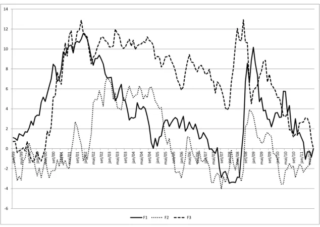
The determination of the number of factors is done using two different criteria: the Kaiser-Guttman and Bai and Ng (2002). In the first criterion, we consider only factors whose associated eigenvalues are larger than 1. In the Bai and Ng (2002) criterion the number of factors is chosen to minimize a loss function based on mean square deviations of the changes of the exchange rate and the estimated factors. Results show that both criteria indicate that N=3 factors are driving the dynamics of the exchange rate in our sample.11 Figure 1 shows the trajectory of the estimated factors.
Figure 1: Evolution of the Common Factors
-6 -4 -2 0 2 4 6 8 10 12 14
jan/99 mai/99 set/99 jan/00 mai/00 set/00 jan/01 mai/01 set/01 jan/02 mai/02 set/02 jan/03 mai/03 set/03 jan/04 mai/04 set/04 jan/05 mai/05 set/05 jan/06 mai/06 set/06 jan/07 mai/07 set/07 jan/08 mai/08 set/08 jan/09 mai/09 set/09 jan/10 mai/10 set/10 jan/11 mai/11
F1 F2 F3
Figure 1 refers to the evolution of the estimated factors. For each country i we have∆sit=µi+ Σ3
j=1δij+vit. The factors shown are cumulated from first differences. The estimates follow the standard case for this study using 152 monthly samples and 18 exchange rates, and the factors are estimated by maximum likelihood.
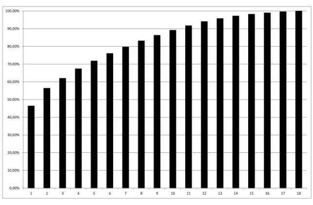
Figure 2 shows the percentage of the variance of the exchange rate that is cumulatively explained by the firstnestimated factors for the complete sample (1999-2011). The figure indicates that the first three factors jointly explain approximately 62% of the variability in the data, with the three factors explaining, respectively, 46%, 10% and 6% of the variability in the data.
Figure 2: Analysis of the Factors
0,00% 10,00% 20,00% 30,00% 40,00% 50,00% 60,00% 70,00% 80,00% 90,00% 100,00%
1 2 3 4 5 6 7 8 9 10 11 12 13 14 15 16 17 18
Figure 2 shows cumulative variance explained by the firstnfactors for the complete sample (1999-2011). Factors are estimated by maximum likelihood withn= 18
factors. The complete sample, consisting of 18 exchange rates and 152 months, is used.
4. IDENTIFICATION OF THE COMMON FACTORS
One of the main criticisms of factor models is that in most cases the estimated factors lack an economic interpretation. This identification is important since it can help in improving the theoretical macroeconomic models that are traditionally used to study the exchange rate determination.
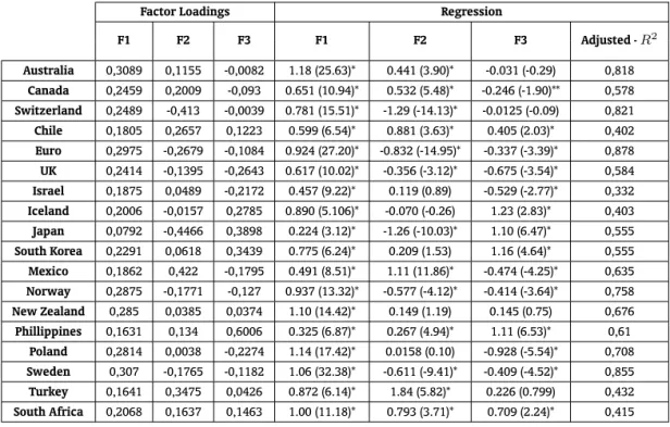
Usually the literature tries to identify the factors through the inspection of the estimated loadings. Initially, we follow this procedure. Results in table 1 indicate that the factor 1 has significant and positive loadings in all of the currencies used. The factor is a weighted mean of all of the exchange rates. This fact allows us to interpret the factor as reflecting the common movements of the currencies with respect to the reference currency. Therefore, factor 1 can be viewed as indicating the strength (weakness) of the dollar against the average of the other currencies - a Dollar effect.
Table 1: Identification of the Common Factors
Factor Loadings Regression
F1 F2 F3 F1 F2 F3 Adjusted -R2
Australia 0,3089 0,1155 -0,0082 1.18 (25.63)* 0.441 (3.90)* -0.031 (-0.29) 0,818
Canada 0,2459 0,2009 -0,093 0.651 (10.94)* 0.532 (5.48)* -0.246 (-1.90)** 0,578
Switzerland 0,2489 -0,413 -0,0039 0.781 (15.51)* -1.29 (-14.13)* -0.0125 (-0.09) 0,821
Chile 0,1805 0,2657 0,1223 0.599 (6.54)* 0.881 (3.63)* 0.405 (2.03)* 0,402
Euro 0,2975 -0,2679 -0,1084 0.924 (27.20)* -0.832 (-14.95)* -0.337 (-3.39)* 0,878
UK 0,2414 -0,1395 -0,2643 0.617 (10.02)* -0.356 (-3.12)* -0.675 (-3.54)* 0,584
Israel 0,1875 0,0489 -0,2172 0.457 (9.22)* 0.119 (0.89) -0.529 (-2.77)* 0,332
Iceland 0,2006 -0,0157 0,2785 0.890 (5.106)* -0.070 (-0.26) 1.23 (2.83)* 0,403
Japan 0,0792 -0,4466 0,3898 0.224 (3.12)* -1.26 (-10.03)* 1.10 (6.47)* 0,555
South Korea 0,2291 0,0618 0,3439 0.775 (6.24)* 0.209 (1.53) 1.16 (4.64)* 0,555
Mexico 0,1862 0,422 -0,1795 0.491 (8.51)* 1.11 (11.86)* -0.474 (-4.25)* 0,635
Norway 0,2875 -0,1771 -0,127 0.937 (13.32)* -0.577 (-4.12)* -0.414 (-3.64)* 0,758
New Zealand 0,285 0,0385 0,0374 1.10 (14.42)* 0.149 (1.19) 0.145 (0.75) 0,676
Phillippines 0,1631 0,134 0,6006 0.325 (6.87)* 0.267 (4.94)* 1.11 (6.53)* 0,61
Poland 0,2814 0,0038 -0,2274 1.14 (17.42)* 0.0158 (0.10) -0.928 (-5.54)* 0,708
Sweden 0,307 -0,1765 -0,1182 1.06 (32.38)* -0.611 (-9.41)* -0.409 (-4.52)* 0,855
Turkey 0,1641 0,3475 0,0426 0.872 (6.14)* 1.84 (5.82)* 0.226 (0.799) 0,432
South Africa 0,2068 0,1637 0,1463 1.00 (11.18)* 0.793 (3.71)* 0.709 (2.24)* 0,415
Table 1 shows the loadings of each estimated factor and the results from the estimation of the following equation∆Sit=µi+ Σ
3
j=1δij+vitfor each countryi, in whichFjtare the three estimated common factors. *, **and *** represent, respectively, 1%, 5% and 10% levels of significance. t-statistics are in parenthesis.
In addition to the loadings, Table 1 also shows the results of the estimation of (1) for each country for a model containing only the estimated factors. Results for factor 1 confirm that this factor represents a “dollar effect”. Factor 1 has a positive and statistically significant impact on all currencies. It is interesting to reinforce that factor 1 accounts for almost 50% of the variability of the exchange rates in the sample, as shown in figure 2.
The analysis for factor 2 indicates a division of the impact of common shocks in two different groups of countries: developed and developing countries. Results in table 1 show that developed countries present a negative loading (and statistically significant impact) with Japanese yen and Swiss franc hav-ing the highest (negative) impact and the Mexican Peso and Turkish Lira presenthav-ing the highest (posi-tive) loadings and estimated coefficients in the regression. These results might indicate that this factor represents a possible “flight to quality” in moments of turmoil when capital flows from developing to developed countries and we observe a disparity in the movements of the exchange rate.
The analysis of factor 3 is more emblematic with respect to the difficulties in using only the analysis of the loadings for assigning an economic interpretation for the common factors. It is not possible to verify any clear pattern among the loadings or in the coefficients that result from the estimation of (1) for each country. Very dissimilar countries with respect to economic development have similar signs making its interpretation a difficult task.
in the economic interpretation of the factors, might reinforce a possible advantage of the use of factor models, that is, the concentration of the information set into a small number of factors.
The empirical literature identifies different variables as correlated with common factors that have an impact in the trajectory of the exchange rate. Cayen et al. (2010), using a similar factor analysis, verify a correlation between commodity prices and common global factors. We use the CRB - Commodity Index in order to analyze this relationship.
McGrevy et al. (2012) identifies the euro/dollar, yen/dollar, and swiss-franc/dollar as the common factors. They argue that the first two exchange rates are the two highest volume of foreign exchange transactions in the spot markets and the Japanese yen and Swiss franc serve as “safe-haven” currencies in moments of turmoil in the U.S. Considering that anecdotal evidence indicates a correlation between gold prices and moments of turmoil, since gold is also viewed as a safe-haven in moments of turmoil in financial markets, we analyze the correlation between gold-prices and the factors. Market participants use the High-yield spread as a proxy for risk aversion. Higher spreads indicate a lower desire by investor to bear risks. Hence, we include the high yield spread in the analysis.
Lustig et al. (2011) found that a ’slope’ effect account for more of the cross-sectional variation in average excess returns between high and low interest rate currencies. They relate these factors to global equity market volatility. In a similar way, Menkhoff et al. (2012) found that global foreign ex-change volatility risk accounts for the highest explanation of cross-sectional excess returns of carry trade portfolios and that liquidity risk also play a role in the explanation of their foreign exchange ex-pected returns. By constructing a measure of FX global liquidity, Banti et al. (2012) show that there is a link between liquidity across currencies and that liquidity risk is priced in the cross section of currency returns.
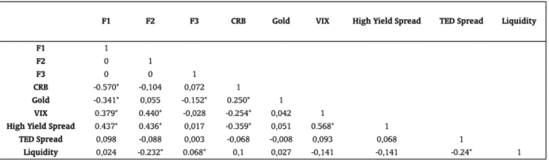
Given the possible role of common volatility and liquidity shocks in the dynamics of the exchange rate we analyze the correlation between the factors and different proxies for these common shocks. The VIX - the Chicago Board Options Exchange Market Volatility Index, a measure of the implied volatility of S&P 500 index options, is used as our proxy for global volatility. For liquidity shocks we use the TED spread and the stock market liquidity measure constructed by Pastor and Stambaugh (2003). Table 2 reports the correlation matrix between the factors and all variables.
Table 2: Correlation Common Factors and Observable Variables
F1 F2 F3 CRB Gold VIX High Yield Spread TED Spread Liquidity
F1 1
F2 0 1
F3 0 0 1
CRB -0.570* -0,104 0,072 1
Gold -0.341* 0,055 -0.152* 0.250* 1
VIX 0.379* 0.440* -0,028 -0.254* 0,042 1
High Yield Spread 0.437* 0.436* 0,017 -0.359* 0,051 0.568* 1
TED Spread 0,098 -0,088 0,003 -0,068 -0,008 0,093 0,068 1
Liquidity 0,024 -0.232* 0.068* 0,1 0,027 -0,141 -0,141 -0.24* 1
Table 2 shows the correlation between the estimated common factors and some observable variables proxies for common shocks (all variables in log-differences). CRB is the CRB commodity price index. Gold stands for the spot gold prices. VIX stands for the Chicago Board Options Exchange Market Volatility Index, a measure of the implied volatility of S&P 500 index options. High Yield Spread is the Merrill Lynch US High Yield Spread. TED Spread is calculated as the difference between the interest rates on interbank loans and on short-term U.S. government debt. Liquidity is the stock market liquidity calculated by Pastor and Stambaugh (2003). * represents 5% level of significance.
The results indicate that factor 1 is highly correlated with the price of commodities. This is in line with the interpretation that factor 1 represents the strength of the reference currency - the American dollar. Since the prices of these commodities are quoted in U.S. dollars, they are tied up with the movements of the dollar compared to other currencies, explaining this high correlation between the factor and the price of commodities.
In contrast, factor 2 has a correlation with the price of the commodities that is lower than factor 1’s. Corroborating the idea that factor 2 might represent the impact of the investors’ perception of the risk in the dynamics of the exchange rate, this factor has higher correlation with the VIX and the high yield spread - the variables that are usually adopted by market participants as measures of risk or investors’ risk aversion. Finally, consistent with the previous analysis, unlike the other two factors, factor 3 is not highly correlated with any variable, and the highest correlations are with the price of gold and with the liquidity measure.12
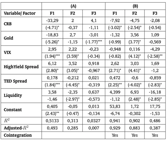
Table 3 shows the results of a more formal analysis between the relationship between the factors and the observable variables. The results of two types of estimations are shown in table 3. In Panel A the common factors and the variables are in (log-) differences, yet in panel B we look for the existence of a long-run relationship between the factors and our proxies for common shocks; therefore, in this case we use the variables in levels and perform a dynamic OLS estimation in order to capture this relationship.
Results in table 3 confirm that there is a relationship between the first factor and the price of commodities. For all of the specifications there is a significant relationship between the first factor and the CRB Index. It is interesting to note that although the high yield spread and the TED spread play a role in the dynamics of the factor, almost all explanatory power of the observable variables comes from the Commodity index.
Results in table 3 indicate that factor 2 carries information related to volatility and liquidity shocks. In both specifications, the VIX, the high yield spread, the TED spread, and the liquidity variable present a robust and statistically significant relationship with the factor - although the liquidity shows a different sign depending on the specification. When we analyze the separate impact of each variable we get that the high yield spread accounts for the bulk of the variability of the factor.
When we observe theR2of each specification we verify that the variables used in the specifications
account for a significant proportion of the variability of the factors in the case of factors 1 and 2, but this is not the case for factor 3. Corroborating previous results, the identification of factor 3 is a more complex task. Results show that the factor is correlated with the gold prices, the VIX, and the proxies for liquidity, but none of the results are robust. In addition, the specifications for the factor present the lowestR2among all specifications.
In summary, the results indicate that the three estimated factors are able to condense information embedded in several variables related to different global shocks and which are advocated by the litera-ture as playing a role in the dynamics of the exchange rate but that are not direct observable by market participants. Therefore, the condition that the information embedded in the common movements of the exchange rates of various countries is related to the unobservable variables is satisfied by the estimated factor. In the next section, we verify the predictive power of the factors.
12One limitation from assigning the significance of the factors using this methodology is that one variable might proxy different
Table 3: Results for the Identification of the Common Factors
(A) (B)
Variable/ Factor F1 F2 F3 F1 F2 F3
CRB -33,29 2 4,1 -7,92 -4,75 -2,08
(-4.71)* -0,37 -1,11 (-3.02)* (-2.54)* (-0.54)
Gold -18,83 2,7 -3,01 -1,32 3,56 1,09
(-5.26)* -1,15 (-1.77)*** (-0.99) (3.77)* -0,569
VIX 2,95 2,22 -0,23 -0,948 0,116 -4,29
(1.94)*** (3.59)* (-0.34) (-0.82) (4.12)* (-2.58)**
HighYield Spread 6,12 3,52 0,918 2,62 3,03 1,69
(2.80)* (3.05)* -0,967 (2.71)* (4.41)* -1,2
TED Spread 0,178 -0,212 0,021 0,472 -0,6 -0,859 (1.84)*** (-4.45)* -0,319 (2.25)** (-4.02)* (-2.83)*
Liquidity 3,58 -2,35 0,637 4,399 6,93 -16,18
-1,46 (-2.97)* -0,573 -1,12 (2.48)* (-2.85)*
Constant 0,405 -0,05 0,013 53,83 1,72 17,75
(2.43)** (-0.47) -0,134 -6,74 -0,302 -1,53
R2 0,5133 0,313 0,0327 0,941 0,902 0,486
Adjusted-R2 0,493 0,285 0,007 0,929 0,883 0,387
Cointegration Yes Yes Yes
Table 3 shows the results for the identification of the common factors. CRB is the CRB commodity price index. Gold stands for the spot gold prices. VIX stands for the
Chicago Board Options Exchange Market Volatility Index, a measure of the implied volatility of S&P 500 index options; High Yield Spread is the Merrill Lynch US High Yield
Spread. TED Spread calculated by the difference between the interest rates on interbank loans and on short-term U.S. government debt. Liquidity is the liquidity proxy
calculated by Pastor and Stambaugh (2003). In panel A all variables are in (log-) differences. Panel B performs the analysis in a cointegration framework performing the
estimation by dynamic OLS with a inclusion of 1(one) lag. Cointegration stands for the Engle-Granger cointegration test. *,** and *** represent, respectively, 1%, 5% and 10%
level of significance. t-statistics in parenthesis.
5. EXCHANGE RATE PREDICTABILITY AND THE COMMON FACTORS
In order to test the predictability of exchange rate models the literature usually performs two types of tests: in-sample and out-of-sample tests. As discussed in Chen et al. (2010), the two sets of tests not rarely produce different results. These results will depend on several aspects like the stability of the pa-rameters, sample size, among others. The authors discuss that in-sample exercises have the advantage of make use of the full sample size, present higher power if the parameters are constant, and are more likely to detect predictability, but these exercises are more prone to overfitting and sometimes fail to present out-of-sample predictability. In opposition, out-of-sample exercises would be more realistic and more robust to time variation and misspecification problems. Considering these facts, in this section, we perform the two types of exercises with the objective of analyzing the usefulness of the common factors in explaining the dynamics of the exchange rate.
table 4 reports the results for the Augment Dickey-Fuller test (ADF), and for the Kwiatkowski-Phillips-Schmidt-Shin (KPSS) unit root test.
Table 4: Unit Root Tests
Variable / Unit Root Test ADF KPSS Exchange Rate -7.30* 0.052+
F1 -10.52* 0.074+
F2 -10.76* 0.063+
F3 -11.25* 0.033+
Brazil
Money Supply -17.47* 0.041+ Industrial Production -6.53* 0.055+ Price Level -5.08* 0.094+
U.S.
Money Supply -11.53* 0.184++ Industrial Production -3.24** 0.064+ Price Level -8.14* 0.065+
Table 4 shows the results for the unit root tests for all variables in log-differences used for the estimation of equation (1). ADF stands for the Augmented Dickey-Fuller test
with null hypothesis that the variable has a unit root. KPSS is the Kwiatkowski-Phillips-Schmidt-Shin test whose null is that the variable is stationary. *, ** indicates the
rejection of the null hypothesis for 1% and 10% critical levels, respectively. + and ++ is placed where the null is not rejected for 1% and 10% critical levels, respectively.
The results in table 4 give strong evidence in favor of the stationarity of the series. Considering a critical value of 10%, the ADF test rejects the presence of a unit root in all variables and only for the industrial production in the U.S. is the null not rejected for a critical value of 1%. Similar results are obtained when using the KPSS test. For a critical value of 10%, the null that the variable is stationary is not rejected for all variables and considering a critical value of 1% the null is only rejected for the money supply in the U.S. Therefore, there is evidence that a specification like (1) is appropriate for the analysis.
5.1. In-sample Predictability
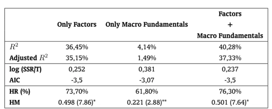
Table 5 shows the result of a set of in-sample tests.13 Results in table 5 indicate that the inclusion
of the factors significantly improve the exchange rate model that contains only macroeconomic fun-damentals. The R2 of the model containing only the macroeconomic variables is 4.14%. This value
increases to 40.28% when the three common factors are included in the model. It is worth noting that the model containing only the estimated factors explains a greater proportion of the changes in the exchange rate than the macro-fundamentals model. TheR2of the factor-model is 36.45%, which
is substantially higher than the R2 of the model enclosing only the macro-fundamentals. A similar
picture emerges when we use the adjusted-R2 as a measure of comparison among the models. The
adjusted-R2increases from 1.49% in the model with only the macro variables to 37.33% when we add
the estimated common factors.
Table 5: In-sample Tests
Only Factors Only Macro Fundamentals
Factors +
Macro Fundamentals
R2 36,45% 4,14% 40,28%
AdjustedR2 35,15% 1,49% 37,33%
log (SSR/T) 0,252 0,381 0,237
AIC -3,5 -3,07 -3,5
HR (%) 73,70% 61,80% 76,30%
HM 0.498 (7.86)* 0.221 (2.88)** 0.501 (7.64)*
Table 5 shows the results of a set of in-sample tests. Results are from the estimation of (1) including only the estimated common factors (Only Factors), only the
macroeco-nomic fundamentals (Only Macro Fundamentals) and with the two set of variables together (Factors + Macro fundamentals). Log (SSR/T) is the logarithm of the sum of the
square of the residuals, AIC is the Akaike information criteria. HR is the percentage of time that the estimated model correctly predicts the realized change in the exchange
rate. HM is the result of the Henriksson and Merton (1981) test. *, ** mean, respectively, 1% and 5% levels of significance.
The results presented in table 5 using the information criteria confirm that the inclusion of the estimated common factors considerably improve the predictive power of the model containing only the macroeconomic fundamentals. Both - the logarithm of the sum of the square of the residuals and the Akaike criteria - present better values for the models that include the factors than for the models that comprise only the macro variables.
Finally, following Fratzscher et al. (2012) we perform two different tests to analyze the market timing capability of the models. The hit ratio test (HR) show the percentage of time that the estimated model correctly predicts the realized change in the exchange rate. The HM Test is a test proposed by Henriksson and Merton (1981) to test the market timing ability of a model. The test estimates the correlation between the realized and fitted exchange rate returns. A positive coefficient can be interpreted as the market timing ability of the model.
The results of the market timing ability test shown in table 5 confirm the superior performance of the models containing the estimated factors. A model containing only the macroeconomic fundamen-tals is able to correctly predict the exchange rate change in 61.8% of the time of the sample, in contrast by adding the estimated factors we are able to predict correctly in 76.3% of times. In addition, the anal-ysis of the coefficients of the HM model also point out the higher predictive power of the models with the factors. Besides being positive and statistically significant, indicating the market timing ability of the models, the coefficients in the models with the factors are higher compared to the coefficients in the benchmark model containing only the macroeconomic fundamentals.
5.1.1. Granger Causality
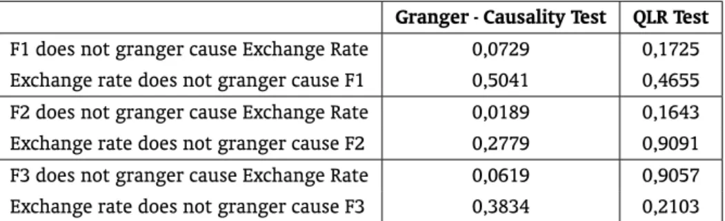
The view that the exchange rate is determined by the present value of future fundamentals makes the Granger causality test a useful tool in analyzing the predictive power of the estimated factors. If the common global factors have any predictability over the exchange rate movements one should fail to reject that the estimated factors granger cause the exchange rate.
table 6 indicate that the hypothesis that the factors do not granger cause the exchange rate is rejected for all three factors. In addition, the results show that the hypothesis that the exchange rate does not Granger cause the factor is not rejected for all three factors. These results confirm the in-sample predictive power of the common global factors.
Table 6: Granger Causality and Stability Tests
Granger - Causality Test QLR Test
F1 does not granger cause Exchange Rate 0,0729 0,1725
Exchange rate does not granger cause F1 0,5041 0,4655
F2 does not granger cause Exchange Rate 0,0189 0,1643
Exchange rate does not granger cause F2 0,2779 0,9091
F3 does not granger cause Exchange Rate 0,0619 0,9057
Exchange rate does not granger cause F3 0,3834 0,2103
Table 6 shows the results (p-value) of the Granger causality tests between the estimated factors and the exchange rate R$ / US$ in the period between January 1999 and
August 2011. The test is performed using heteroskedasticity and autocorrelation robust variance estimation (Newey and West, 1987). Table 6 also reports the p-values for
the Andrews stability test.
Several authors (Chen et al. (2010), Rossi (2006, 2012), among others) argue that the difficulty in modeling the dynamics of the relationship between the exchange rate and the macroeconomic funda-mentals is that for different reasons this relationship is unstable over time. Rossi (2005) discusses that conventional Granger causality test fail in the presence of these instabilities. In order to analyze this problem, table 6 also reports results from Quandt Likelihood Ratio (QLR) instability tests (Andrews, 1993) for the Granger-causality relationship between the factors and the exchange rate. The results indicate that for any of the relationships analyzed the tests reject the presence of instabilities, strengthening the results from the Granger causality tests.
In summary, all in-sample exercises indicate that the inclusion of the estimated common factors improves the predictive power of the traditional macroeconomic models and that, unlike the relation-ship between the exchange rate and the macroeconomic fundamentals, the role of the common factors in the exchange rate dynamics seem to be more stable. Next section analyzes whether this in-sample improvement is also translated in a better out-of-sample predictability.
5.2. Out-of-sample Predictability
We follow Ferraro et al. (2012) and perform a rolling windows “out-of-sample” forecasting exercise using equation (1). Chen et al. (2010) argue that the rolling window scheme is more robust with respect to a possible time-variation of the parameters because it adapts more quickly to possible structural changes when compared to a recursive scheme. Yet, we include the use of different methodologies, like the recursive scheme, as robustness exercises. The out-of-sample forecast is done for four different forecast horizons (h=1, 3, 6 and 12 months ahead).
The process of out-of-sample forecasting is executed according to the following steps for a sample sizeT=152 months. Starting in January 1999, for a given window size (N) and a forecast horizon (h), the factors are estimated from the series of the exchange rate of the 18 countries, using the maximum likelihood method, as follows:
In the second step, equation (1) is estimated using the factors estimated in the first step and/or macroeconomic fundamentals using only data until time t. Given the estimation of (1), a h-period ahead forecast is performed. The process is done for all forecast horizons h=1,3 ,6 and 12 months ahead. Then we advance one-period and the forecasting is performed again. We continue until the end of the sample.
Here a very important remark has to be made. The forecast exercise performed is not a real “out-of-sample” forecast exercise. Note that according to (2), data untilt+his used in order to estimate the factors; therefore, in the forecasting process, realized values for the factors and the macroeconomic fundamentals are used. West (1996) points out that this type of exercise is useful for the evaluation of the predictability of a model given the path of the variables.
Ferraro et al. (2012) argue that if the goal of the exercise is to demonstrate the usefulness of the addition of a fundamental - in our case, the common factors - this forecasting strategy would be more appropriate. In their case, they advocate this strategy given the difficult in forecasting oil prices - their additional fundamental. They discuss that if past values of oil prices are not good predictors of future oil prices one might reject the predictability of the model due to poor forecast process that past oil prices give for future oil prices and not because of the lack of relationship between the exchange rate and the additional fundamental.
It is clear that in our case this problem is even more pronounced given that we do not have any formal model to forecast the factors. Given these facts, we use the rolling “out-of-sample” forecast exercise as our baseline strategy and leave the other strategies to be analyzed as robustness exercises. The out-of-sample forecasting (described above) is then compared with a forecast model that assumes that the exchange rate follows a random walk with and without a drift.
We use the Theil’s U statistic as the criterion for judging the performance of each model. The statistic is calculated as the ratio between the mean square prediction error (MSPE) of each model and the mean square prediction error of the two different benchmark models: random walk with and without a drift. Values lower than 1 indicate that the model possesses a MSPE smaller than that of the random walk model. However, even a value higher than 1 can be considered evidence of a superior performance of the model compared to the random walk. As argued in Clark and West (2006), Clark (2007), if the process generating the exchange rate is, in fact, a random walk, the inclusion of other variables should introduce noise in the forecasting process, leading, on average, to a mean square prediction error greater than that of the random walk (and thus producing statistics with a value greater than 1).
We then use the Clark and West (2006) statistic as the evaluation criterion for forecast quality. The Clark and West (2006) is more appropriate for asymptotic tests than the one given by Diebold and Mar-iano (1995) and West (1996) (DMW) for nested models. As observed by Clark and West (2006), in nested models, the DMW statistics yield a test statistic with a non-normal distribution, which underestimates the quantity of null hypothesis rejections.
5.2.1. Baseline Results
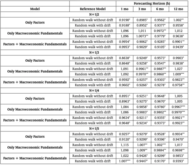
Table 7 confirms the usefulness of the estimated common factors in improving the predictive power of the models containing only macroeconomic fundamentals. When we analyze the predictive power of the models containing only the macroeconomic variables we verify the conventional instability found by the literature. Although the model is able to beat the random walk in several occasions, it does not do this in a robust manner. In all specifications, for example, the model is not able to beat for short-horizon forecasts (1-month ahead). The model containing only macroeconomic fundamentals seems to have more predictive power for medium and long-horizon forecasts, although even for these forecast horizons the model is not able to beat the random walk benchmark in different opportunities.
walk in short-horizons forecasts but there is also a significant reduction in the mean square predic-tion error of the model, confirming that the common factors carry useful informapredic-tion for forecasting the exchange rate. In fact, for almost all forecast horizons and sample size a model containing the macroeconomic fundamentals together with the estimated factors is able to beat the two benchmark models.
The usefulness of the estimated factors for short-term predictions is evident when we analyze the model containing only these fundamentals. The model containing only the factors presents the lowest mean square error predictions for all specifications. It is interesting to note that the model containing only the factors is also able to beat the benchmark models in almost all specifications, assuring the importance of these factors in the dynamics of the exchange rate.
Table 7: Forecasting Results
Forecasting Horizon (h)
Model Reference Model 1 mo 3 mo 6 mo 12 mo
N=1/2
Only Factors Random walk without drift 0.9190* 0.8985* 0.9562* 1.002**
Random walk with drift 0.9188* 0.8952* 0.9377* 0.9558*
Only Macroeconomic Fundamentals Random walk without drift 1,096 1,011 0.9972** 1,012
Random walk with drift 1,096 1.0073** 0.9779* 0.9638*
Factors + Macroeconomic Fundamentals Random walk without drift 0.9954* 0.9062* 0.9285* 0.9901**
Random walk with drift 0.9953* 0.9029* 0.9105* 0.9439*
N=1/3
Only Factors Random walk without drift 0.8638* 0.9249* 0.9573* 0.9903*
Random walk with drift 0.8648* 0.9258* 0.9547* 0.9838*
Only Macroeconomic Fundamentals Random walk without drift 1,091 0.9961** 0.9887** 1,027
Random walk with drift 1,092 0.9970** 0.9860** 1.009***
Factors + Macroeconomic Fundamentals Random walk without drift 0.9592* 0.9257* 0.9303* 0.9823**
Random walk with drift 0.9602* 0.9266* 0.9278* 0.9758**
N=1/4
Only Factors Random walk without drift 0.8951* 0.9251* 0.9648* 1,005
Random walk with drift 0.8963* 0.9275* 0.9670* 1,005
Only Macroeconomic Fundamentals Random walk without drift 1,084 0.9858* 0.9780* 0.9967***
Random walk with drift 1,086 0.9883* 0.9802** 0.9970***
Factors + Macroeconomic Fundamentals Random walk without drift 0.9634* 0.9211* 0.9355* 0.9921**
Random walk with drift 0.9648* 0.9234* 0.9373* 0.9923**
N=1/5
Only Factors Random walk without drift 0.9257* 0.9279* 0.9528* 0.9934**
Random walk with drift 0.9120* 0.9299* 0.9396* 0.9470*
Only Macroeconomic Fundamentals Random walk without drift 1,115 1.007** 1.002*** 1,017
Random walk with drift 1,098 1.009** 0.9884** 0.9698**
Factors + Macroeconomic Fundamentals Random walk without drift 1,022 0.9426* 0.9299* 0.9853*
Random walk with drift 1.007*** 0.9447* 0.9170* 0.9393*
5.2.2. Alternative Specifications
Results found in table 7 might be the due to the specification adopted. In order to verify the strength of the results we perform several robustness exercises.
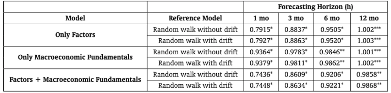
5.2.2.1. Recursive (Sequential) Strategy In this exercise we follow procedures similar to the baseline framework, but now instead of rolling the estimation window we add one observation one by one until the end of the sample. Each observation is included in the sample such that the sample available for estimations of the regression and factors increases. In this case, we start with a sample size that is 1/5 of the full sample. The results in table 8 confirm our previous findings with respect to the usefulness of the common factor in predicting the exchange rate. The results in table 8 indicate that the use of both fundamentals - common factors and macroeconomic - leads to better results. Although all models are able to beat the benchmark models, the combination of the models gives the best result, with lower mean square prediction errors for all forecast horizons.
Table 8: Robustness Exercises
Forecasting Horizon (h)
Model Reference Model 1 mo 3 mo 6 mo 12 mo
Only Factors Random walk without drift 0.7915* 0.8837* 0.9505* 1.002***
Random walk with drift 0.7927* 0.8863* 0.9520* 1.003***
Only Macroeconomic Fundamentals Random walk without drift 0.9364* 0.9783* 0.9846** 1.001***
Random walk with drift 0.9379* 0.9811* 0.9862** 1.002***
Factors + Macroeconomic Fundamentals Random walk without drift 0.7436* 0.8609* 0.9206* 0.9858**
Random walk with drift 0.7448* 0.8634* 0.9221* 0.9868**
Table 8 shows the Theil’s U statistic defined as the ratio between the mean square prediction error of a model and that given by two different benchmark models: the random walk with and without a drift. Asterisks represent the result of the Clark and West (2006) test statistic. *, **and *** represent, respectively, p-values for the test lower than 1%, 5% and 10%. The complete sample corresponds to the period from January 1999 to August 2011 and consists of 152 monthly observations.
5.2.2.2. Lagged The rolling “out-of-sample” strategy adopted is not a truly out-of-sample exercise since it uses realized fundamentals. This strategy is of limited use to professional forecasters since it makes use of information not available to the forecaster. Now we consider the following change in equation (1) for any forecast horizon h:
∆St=α+β.Ft−h+γ.Zt−h+ut (3)
Observe that now only the lagged value of the estimated common factors and the macroeconomic fundamentals are used in order to forecast the exchange rate. Following this procedure, the forecast process is performed using only information available at timet. The other procedures are similar to the exercises done for the baseline framework. The results for a sample size N= 1
2 of the total sample is
shown in table 9.14
14The results are unchanged with respect to the sample size. In order to save space they are not shown but are available upon
Table 9: Robustness exercises
Forecasting Horizon (h)
Model Reference Model 1 mo 3 mo 6 mo 12 mo
N=1/2
Only Factors Random Walk without drift 0.9299* 0.9662* 0.9893** 0.9566*
Random walk with drift 0.9298* 0.9633* 0.9722* 0.9440*
Only Macroeconomic Fundamentals Random Walk without drift 1,009 0.9772* 1.007*** 0.9774*
Random walk with drift 1,009 0.9743* 1.006*** 0.9352*
Factors + Macroeconomic Fundamentals Random Walk without drift 0.9721* 0.9600* 0.9724* 0.9513*
Random walk with drift 0.9721* 0.9571* 0.9556* 0.9389*
Table 9 shows the Theil’s U statistic defined as the ratio between the mean square prediction error of a model and that given by two different benchmark models: the random walk with and without a drift. Asterisks represent the result of the Clark and West (2006) test statistic. *, **and *** represent, respectively, p-values for the test lower than 1%, 5% and 10%. The complete sample corresponds to the period from January 1999 to August 2011 and consists of 152 monthly observations. Exercise is performed for a window size equals to1
2of the full sample.
The results in table 9 confirm the robustness of the previous analysis. Both - the model contain-ing the factors and the macroeconomic variables - are able to beat the two benchmark specifications, with the model using only the macroeconomic fundamentals demonstrating more difficulty to beat the benchmark models, especially for short forecast horizon. This problem seems to be solved once we add the estimated factors. The model containing both the macroeconomic fundamentals and the estimated factors is able to beat the random walk benchmarks for any forecast horizon, assuring that the factors carry useful information for forecasting the exchange rate.
6. CONCLUSIONS
This paper studies the usefulness of the use of factors embedded in the common movements of exchange rates in forecasting the exchange rate of the Brazilian Real / US Dollar from January 1999 to August 2011. The results confirm that the inclusion of the common factors improves the in-sample and out-of-sample predictability of traditional models for the determination of the exchange rate that includes only macroeconomic fundamentals.
In the case of the out-of-sample exercise, the paper shows that, independently of the forecast hori-zon or window of estimation, a model including the estimated common factors and the macroeconomic fundamentals is able to beat any of the benchmark models considered - the random walk with or with-out a drift. The results are even more pronounced for short term predictions - a recurrent failure of the traditional models.
The paper also tries to link the factors to observable variables usually considered by market partic-ipants and the literature as proxies for common global shocks. The results indicate that the estimated factors condense the information contained in a set of variables. The estimated factors carry informa-tion on the demand for dollars - a dollar effect, global volatility and liquidity shocks.
BIBLIOGRAPHY
Bacchetta, P. & van Wincoop, E. (2011). On the Unstable Relationship between Exchange Rates and Macroeconomic Fundamentals. Mimeo.
Bacchetta, P. & van Wincoop, E. (2004). A Scapegoat Model of Exchange Rate Determination. American Economic Review, Papers and Proceedings, 94:114–118.
Bacchetta, P. & van Wincoop, E. (2006). Can Information Heterogeneity Explain the Exchange Rate Determination Puzzle? American Economic Review, 96:552–576.
Bai, J. (2004). Estimating Cross-Section Common Stochastic Trends in Nonstationary Panel Data.Journal of Econometrics, 122:137–183.
Bai, J. & Ng, S. (2002). Determining the Number of Factors in Approximate Factor Models. Econometrica, 70:191–221.
Banti, C., Phylactis, K., & Sarno, L. (2012). Global liquidity risk in the foreign exchange market. Journal of International Money and Finance, 31:267–291.
Bekaert, G., Hoerova, M., & Duca, M. (2010). Risk, uncertainty and monetary policy. Working Paper 16397, NBER .
Cayen, J., Coletti, D.and Lalonde, R., & Maier, P. (2010). What Drives Exchange Rates? New Evidence from a Panel of U.S. Dollar Bilateral Exchange Rates. Working Paper 2010-5, Bank of Canada.
Chen, Y. & Rogoff, K. (2003). Commodity Currencies.Journal of International Economics, 60:133–169. Chen, Y., Rogoff, K., & Rossi, B. (2010). Can exchange rates forecast commodity prices? Quarterly Journal
of Economics, 125:1145–1194.
Cheung, Y., Chinn, M., & Pascual, A. b. (2005). What Do We Know about Recent Exchange Rate Models? In-Sample Fit and Out-of-Sample Performance Evaluated. in Paul De Grauwe, ed., Exchange Rate Economics: What Do we Stand?, The MIT Press: Chapter 8, 239-76.
Chinn, M. & Moore, M. (2010). Order Flow and the Monetary Model of Exchange Rates: Evidence from a Novel Data Set. Mimeo.
Clark, T. & West, K. (2007). Approximately Normal Tests for Equal Predictive Accuracy in Nested Models.
Journal of Econometrics, 138:291–311.
Clark, T. & West, D. (2006). Using Out-of-Sample Mean Squared Prediction Errors to Test the Martingale Difference Hypothesis.Journal of Econometrics, 135:155–186.
Diebold, F. & Mariano, R. (1995). Comparing predictive accuracy. Journal of Business and Economic Statistics, 13:253–263.
Engel, C., Mark, N., & West, K. D. (2008). Factor Model Forecasts of Exchange Rates. Mimeo.
Engel, C. & West, K. (2005). Exchange Rates and Fundamentals.Journal of Political Economy, 113:485–517. Engel, C. & West, K. (2006). Taylor Rules and the Deutschmark-Dollar Real Exchange Rate. Journal of
Money, Credit and Banking, 38:1175–1194.
Evans, M. & Lyons, R. (2005). Meese-Rogoff Redux: Micro-based Exchange Rate Forecasting. American Economic Review, 95:405–414.
Evans, M. & Lyons, R. (2008). How Is Macro News Transmitted to Exchange Rates? Journal of Financial Economics, 88:26–50.
Faust, J., Rogers, J., & Wright, J. (2003). Exchange rate forecasting: the errors we’ve really made.Journal of International Economics, 60:35–59.
Ferraro, D., Rogoff, K., & Rossi, B. (2012). Can oil prices forecast exchange rates? Working Paper 17998, NBER.
Forni, M., Hallin, M., Lippi, M., & Reichlin, L. (2000). The Generalized Dynamic Factor Model: Identifica-tion and EstimaIdentifica-tion. Review of Economics and Statistics, 82:540–554.
Forni, M. & Reichlin, L. (1998). Let’s Get Real: A Factor Analytic Approach to Disaggregated Business Cycle Dynamics. Review of Economic Studies, 65:453–473.
Fratzscher, M., Sarno, L., & Zinna, G. (2012). The scapegoat theory of exchange rates: The first tests. Working Paper 1418, European Central Bank.
Galimberti, J. & Moura, M. (2013). Taylor rules and exchange rate predictability in emerging economies.
Journal of International Money and Finance, 32:1008–1031.
Groen, J. (2005). Exchange Rate Predictability and Monetary Fundamentals in a Small Multi-Country Panel. Journal of Money, Credit and Banking, 37:495–516.
Groen, J. J. (2006). Fundamentals Based Exchange Rate Prediction Revisited. Manuscript, Bank of Eng-land.
Henriksson, R. & Merton, R. (1981). On the Market Timing and Investment Performance of Managed Portfolios II - Statistical Procedures for Evaluating Forecasting Skills. Journal of Business, 54:513–533. Lustig, H., Roussanov, L., & Verdelhan, A. (2011). Common Risk Factors in Currency Markets. Review of
Financial Studies, 24:1–47.
Mark, N. (2008). Changing Monetary Policy Rules, Learning and Real Exchange Rate Dynamics. Manuscript, University of Notre Dame.
Mark, N. & Sul, D. (2001). Nominal Exchange Rates and Monetary Fundamentals: Evidence from a Small Post-Bretton Woods Sample.Journal of International Economics, 53:29–52.
McGrevy, R., Mark, N., D., S., & Wu, J. (2012). Exchange rates as exchange rate common factors. Working paper, George Washington University.
Meese, R. & Rogoff, K. (1983). Empirical Exchange Rate Models of the Seventies: Do They Fit Out of Sample? Journal of International Economics, 14:3–24.
Menkhoff, L., Sarno, L., Schmeling, M., & Schrimpf, A. (2012). Carry Trades and Global Foreign Exchange Volatility. The Journal of Finance, 67:681–718.
Moura, M., Lima, A., & Mendonça, R. (2008). Exchange Rate and Fundamentals: The Case of Brazil.
Revista de Economia Aplicada, 12:395–416.
Pastor, L. & Stambaugh, R. (2003). Liquidity Risk and Expected Stock Returns.Journal of Political Economy, 111:642–685.
Rossi, B. (2005). Testing long-horizon predictive ability with high persistence and the Meese-Rogoff puzzle.International Economic Review, 46:61–92.
Rossi, B. (2006). Are exchange rates really random walks. Macroeconomic Dynamics, 10:20–38.
Rossi, B. (2012). The changing relationship between commodity prices and prices of other assets with global market integration. Mimeo.
Stock, J. H. & Watson, M. (2002). Forecasting Using Principal Components from a Large Number of Predictors.Journal of the American Statistical Association, 97:1167–1179.
A. APPENDIX A – TABLE A.1- DATA DESCRIPTION
Table A-1
Variable Country Description Source
Exchange Rate Switzerland log (Domestic Currency / Foreign Currency) Bloomberg
Exchange Rate Norway log (Domestic Currency / Foreign Currency) Bloomberg
Exchange Rate Euro Zone log (Domestic Currency / Foreign Currency) Bloomberg
Exchange Rate New Zealand log (Domestic Currency / Foreign Currency) Bloomberg
Exchange Rate United Kingdom log (Domestic Currency / Foreign Currency) Bloomberg
Exchange Rate Sweden log (Domestic Currency / Foreign Currency) Bloomberg
Exchange Rate Japan log (Domestic Currency / Foreign Currency) Bloomberg
Exchange Rate Poland log (Domestic Currency / Foreign Currency) Bloomberg
Exchange Rate Canada log (Domestic Currency / Foreign Currency) Bloomberg
Exchange Rate Australia log (Domestic Currency / Foreign Currency) Bloomberg
Exchange Rate Iceland log (Domestic Currency / Foreign Currency) Bloomberg
Exchange Rate South Korea log (Domestic Currency / Foreign Currency) Bloomberg
Exchange Rate South Africa log (Domestic Currency / Foreign Currency) Bloomberg
Exchange Rate Israel log (Domestic Currency / Foreign Currency) Bloomberg
Exchange Rate Mexico log (Domestic Currency / Foreign Currency) Bloomberg
Exchange Rate Chile log (Domestic Currency / Foreign Currency) Bloomberg
Exchange Rate Philippines log (Domestic Currency / Foreign Currency) Bloomberg
Exchange Rate Turkey log (Domestic Currency / Foreign Currency) Bloomberg
Exchange Rate Brazil log (Domestic Currency / Foreign Currency) Bloomberg
Industrial Production Brazil Index Jan 2002=100 with seasonal adjustment IBGE
Industrial Production United States Index Jan 2007=100 with seasonal adjustment Federal Reserve
Prices Brazil IPCA - Index Dec 98=100 IBGE
Prices United States CPI - Index Dec 82=100 BLS
Money Supply Brazil R$ millions with seasonal adjustment Central Bank
Money Supply United States US$ billions with seasonal adjustment Federal Reserve
Figure A-1: Evolution of the Exchange rate Brazilian Real / US$ and the Macroeconomic Fundamentals
Figure A.1 shows the trajectory of the exchange rate Real / US$ and the main macroeconomic fundamentals used in the analysis from January 1999 to August 2011. M1 is