A Two-Sector Growth Model with Endogenous Human Capital and Amenities

A TWO-SECTOR GROWTH MODEL WITH

ENDOGENOUS HUMAN CAPITAL AND AMENITIES

Wei-Bin Zhang

College of Asia Pacific Management, Ritsumeikan Asia Pacific University Oita Prefecture, Japan

Regular article Received: 3. February 2008. Accepted: 21. January 2009.

ABSTRACT

This paper examines issues related to urbanization with labour migration. The main departures from the traditional approaches to dynamics of economic structures are that the paper uses an alternative approach to consumer behaviour and introduces human capital accumulation via learning by doing. The model describes dynamic interactions among agricultural and industrial production, rural and urban amenities, distribution of production factors and preferences with endogenous capital and human capital accumulation. We show that the dynamic system may have either a single or multiple equilibrium points, depending upon returns to scale in the two sectors. We also examined effects of changes in some parameters.

KEY WORDS

two-sector model, agricultural sector, industrial sector, physical capital accumulation, human capital accumulation, rural and urban amenities

INTRODUCTION

It is important to study urbanization with labour migration as in many less developed countries an important part of the population is still devoted to agriculture. In economies like India, China and some African countries, agricultural population shares a high percentage of the total population. On the other hand, industrialization and human capital accumulation are altering dramatically the labour distribution between agricultural and non-agricultural sectors in many developing economies. It is well known that the Harris-Todaro framework has played the role of a key model in analyzing industrialization with labour migration between the urban and rural areas1.The Harris-Todaro model attempts to explain persistent rural-urban migration despite the high unemployment rates in cities, especially in developing economies. In this model, the formal-sector wage is fixed at a level far above the agricultural wage and the migration decision is based on expected earnings. To maintain the presumed equalization of expected earnings, some urban residents are unemployed as migration is costless. The change in the probability of formal employment is the principal mechanism that restores migration equilibrium in response to exogenous changes such as technical progress and job or wage growth in the city. As pointed out by Brueckner and Zenou [1], there are many other factors that limit urban growth. For instance, a rise in the city population raises the urban living cost, mostly likely through the land markets, which limits urban growth. As the urban population rises in response to positive shocks, land prices tend to rise, lowering the utility levels of all urban residents. The gap between rural utility and the expected utility of an urban resident is closed up by migration. This study examines migration equilibrium without unemployment. Although we still assume equalization of utility levels between the urban and rural areas, we analyze differences in urban and rural living conditions by assuming that urban and rural areas offer not only different wage rates but also different levels of amenity. This study shows how productivities, land and amenity interact to determine labour distribution between the urban and rural areas in the long term. By taking account of endogenous amenity and land and human capital accumulation, we try to offer an alternative approach to the economy described by the Harris-Todaro model.

Another important issue related to economic structural change is dynamics of human capital and technological change. It is well known that it is difficult to introduce both human capital and physical capital accumulation as endogenous variables into the Harris-Todaro framework because of analytical intractability. For instance, Matsuyama [2] examines how agricultural productivity influences economic growth and the process of industrialization. The model shows that the effect of agricultural productivity on growth is crucially dependent on openness to trade. Nevertheless, Matsuyama’s analysis relies on the assumption that agriculture is backward and no technological progress will take place in the sector. The growth process is driven solely by learning by doing in manufacturing. Nevertheless, the assumption that human capital accumulation is negligible through learning by doing in agricultural sector is not realistic2. This study takes account of human capital accumulation both in industrial and agricultural sectors. Multiple equilibrium points exist when the two sectors exhibit increasing and decreasing returns to scale. Although our model is constructed in dynamics, because of the nature of the problem, it is difficult to carry out a complete dynamic analysis. This study is mainly concerned with issues of existence of equilibrium and comparative statics analysis.

the traditional approach by proposing an alternative approach to household behaviour. The equilibrium mechanism of labour migration is expressed by equalizing utility levels in the urban and rural areas. Different from the Harris-Todaro approach, we use the concept of amenity to reflect living and work condition differences between the urban and rural areas. The wage rates differ between the industrial and agricultural sectors because the urban and rural areas offer different levels of amenity and land rent. It should be noted that this paper is an extension of a model proposed by Zhang [3; Ch. 6]. The main difference between this model and Zhang’s model is that this study introduces differences in amenity between urban and rural areas, while Zhang’s does not take account of possible differences in amenity in different professions and economic geography. The paper is organized as follows. Section 2 defines the two-sector growth model with physical and human capital accumulation. Section 3 provides the process to determine all the variables and demonstrate existence of equilibrium when the parameter values are specified. Section 4 examines effects of changes in the total productivity, the population, and propensity on the levels of physical and human capital and economic structure. Section 5 concludes the study. Appendix A.1 proves the process of finding equilibrium in Section 3. Appendix A.2 shows how to express the dynamics of the economic variables in a three differential equations system.

ECONOMIC GROWTH WITH PHYSICAL AND HUMAN CAPITAL

ACCUMULATION

Similar to Harris and Todaro [4] and Irz and Roe [5], we consider an economic system consisting of agricultural and industrial sectors. The agricultural sector produces goods such as corn, rice and vegetables, which are only for consumption. The industrial sector produces commodities for investment and consumption. Industrial commodity is selected to serve as numeriare. It is assumed that labour force, land and capital are always fully employed3. The population is assumed to be homogenous in the sense that their preference and skill structures are identical. This implies that people can costlessly move from countryside to city, and vice versa. A person is free to choose his residential location. We assume that any person chooses the same area where he works and lives. Each area has fixed land. Land quality, climates, and environment are homogenous within each area, but they may vary between the areas. We neglect transportation cost of commodities4_{. As become evident later on, although it is conceptually}

not difficult to introduce transportation cost function and to provide balance conditions for demand and supply and for price equalization conditions with transportation cost, the problem will become analytically too complicated. The assumption of zero transportation cost of commodities implies price equality for the commodity over space. Nevertheless, as amenity and land are immobile, wage rates and land rent vary between the areas.

BEHAVIOUR OF PRODUCTION SECTORS

We denote K(t), r(t) and p(t) the total capital, the rate of interest and price of agricultural commodity, respectively. We define the following indexes and variables

a, i – subscripts denoting agriculture and industry,

N – the total fixed labour force of the economy,

Li and L – the fixed urban and rural areas,

Nj(t) and Kj(t) – the labour force and capital stocks employed by sector j (j = a, i) at time t,

La(t) – the land employed by the agricultural sector,

Fj(t) and Cj(t) – sector j’s output and consumption levels of product j, and

We assume that production processes can be described by some aggregate production functions. We assume that agricultural production is a process of combining land, labour force and capital. For simplicity, the production function of the agricultural sector is specified as follows

( )

a t A K H N L m

F a a a a ₍₁₎

Here, the term Hma/βa⋅_N

a is the qualified labour input. The parameter ma/βa describes how effectively the agricultural sector utilizes human capital. The marginal conditions for the agricultural sector are given by

, ,

,

a a a

a a a a a

a a k

L pF R

N pF w

K pF

r +δ =α = β = ς (2)

where δk is depreciation rate of physical capital.

The industrial production is a process of combining labour force and capital. The land use by the industrial sector is omitted5. The production function of the industrial sector is specified as follows

( )

i t AK H N m

F αi i βi βi α β α β ₍₃₎

The marginal conditions for the industrial sector are given by

. ,

i i i i i

i i k

N F w

K F

r +δ =α = β (4)

We described behaviour of the production sectors.

CONSUMER BEHAVIOUR

Each worker may get income from land ownership, wealth ownership and wages. To simplify the model, we accept the assumption of “equally shared landownership” which means that the income of land rent is equally distributed among the population. The total land revenue is given by Ri(t)⋅Li + Ra(t) L, where Ri(t) and Ra(t) are the land rents in the city and the rural area, respectively. Each consumer obtains the following land revenue

( )

( )

( )

N

L t R L t R t

r ≡ i i + a ₍₅₎

This study uses the approach to consumers’ behaviour proposed by Zhang in the early 1990s [3, 6]. This approach makes it possible to solve many national, international, urban, and interregional economic problems, such as growth problems with heterogeneous households, multi-sectors, and preference changes, which are analytically intractable by the traditional approaches in economics. Let k_j(t) stand for the per capita wealth (excluding

land) owned by the typical household j Each household of area j obtains income

( ) ( ) ( )

( ) ( )

y_j = _j + _j + =

( )

( )

( )

ˆ t y t k t

y_j = _j + _j (6)

The disposable income is used for saving and consumption. It should be noted that the value,

)

(t

k_j (i.e., pi(t)kj(t)), in the above equation is a flow variable. Under the assumption that

selling wealth can be conducted instantaneously without any transaction cost, we may consider k_j(t) as the amount of the income that the consumer obtains at time t by selling all of his wealth. Hence, at time t the consumer has the total amount of income equaling ŷj(t) to distribute between consuming and saving. It should also be remarked that in the growth literature, for instance, in the Solow model, the saving is out of the current income, yi(t) while in this study the saving is out of the disposable income. This approach is discussed at length elsewhere [3, 6]6_.

At each point of time, a consumer distributes the total available budget among housing, lj(t) saving, sj(t) consumption of agricultural goods, cja(t) and consumption of industrial goods, cji(t). The budget constraint is given by

. ˆ_j

j ja ji

j

jl c pc s y

R + + + = (7)

Furthermore, at each point of time, consumers have four variables to decide. A consumer decides how much to consume housing, industrial and agricultural goods, and how much to save. Equation (7) means that consumption and savings exhaust the consumers’ disposable personal income.

We assume that utility level, U_j(t), that the consumer j obtains is dependent on lj(t), cj(t),

cja(t) and sj(t). The utility level of the typical consumer in region j is represented by

( )

( ) ( ) ( ) ( ) ( )

U_j =θ_j η_j ξ_j µ_ja λ_j η₀,ξ₀,µ₀,λ₀ >0, j =a,i, (8) in which η0, ξ0, µ0 and λ0 are a typical person’s elasticity of utility with regard to lot size,

industrial goods, agricultural goods, and savings in area j, respectively. We call η0, ξ0, µ0 and

λ0 the propensities to consume lot size, industrial goods, agricultural goods, and to hold wealth (save), respectively. In (8), θa(t) and θi(t) are respectively called the rural and urban amenity levels. Amenities are affected by, for instance, infrastructures, professional. In this study, we assume that amenity is affected by production and consumption activities. We specify θj as follows

( )

( )

j j

j =θ =

θ (9)

where θ_j (>0) and dj are parameters. We do not specify sign of dj as the population may have either positive or negative effects on the attractiveness of a location7_{. Maximizing U}

j(t) subject to the budget constraints yields

( )

, ) ( ˆ ) ( , ) ( ˆ ) ( )

(t R t y t c t y t p t c t y t s t y t

l_{j j} =η _{j j} =ξ _{j ja} = µ _{j j} =λ _j (10)

where

. ) (

, ,

,

, _{0 0 0 0 0 0 0} 1

0

− + + + ≡ ≡

≡ ≡

≡ ρη ξ ρξ µ ρµ λ ρλ ρ η ξ µ λ

η

As shown in [3], the saving behaviour of the approach in this study is similar to these implied by the Keynesian consumption function and permanent income hypotheses, which are

empirically more valid than the assumptions in the Solow model with a constant saving rate or the Ramsey model8_{. It should be remarked that the saving, s(t) defined in this study is different}

According to the definitions of sj(t) the wealth accumulation of the representative household in area j is given by

) ( ) ( )

(t s t k t

k&_j = _j − _j . (11)

As households are assumed to be freely mobile between the two areas, the utility level of people should be equal, irrespective of in which area they live, i.e.

Ui(t) = Ua(t). (12)

We neglect possible costs for migration. In reality, even to change a house in a small town costs. Although it is not difficult to introduce migration costs into the model, it will become far more difficult to explicitly get analytical results. In this study, instead of wage equalization (which is often used as the equilibrium mechanism of population distribution), we assume that consumers obtain the same level of utility in different professions as the equilibrium mechanism of population distribution between the professions. Although the condition of utility equalization is often used in the literature of urban economics, the assumption of utility equalization is not often used in the literature of economic dynamics as the temporary equilibrium condition of population distribution. It is argued that this assumption is more reasonable than the assumption of wage equalization.

The total capital stock employed by the production sectors is equal to the total wealth owned by all the regions. That is

) ( ) ( ) ( ) ( ) ( ) ( )

(t K t K t k t N t k t N t

K = _a + _i = _{a a} + _{i i} . (13)

The national demand for and supply of agricultural goods is equal. That is

) ( ) ( ) ( ) ( )

(t N t c t N t F t

c_{aa a} + _{ia i} = _a (14)

The national production of industrial goods is equal to the national consumption and national net saving. That is

C(t)+S(t) – K(t)+δkK(t)=Fi(t), (15)

where

C(t) ≡ca(t)Na(t) + ci(t)Ni(t), S(t) ≡sa(t)Na(t) + si(t)Ni(t). The assumption that labour force and land are fully employed is represented by

Na(t) + Ni(t) = N, li(t)Ni(t) = Li, La(t) + la(t)Na(t) = L. (16)

HUMAN CAPITAL ACCUMULATION

We assume that there are two sources of improving human capital, through learning by doing10_{. Arrow [7] first introduced learning by doing into growth theory. We specify the}

following dynamics11

H NH

F N NH

F N

H a a a i i i _h

i

a δ

τ τ

δ δ + −

=

& _{, (17)}

We have thus established the economic dynamics with endogenous economic structure, physical capital and human capital. We now examine dynamic properties of the system.

ECONOMIC EQUILIBRIUM

This section shows that the dynamic system may have either a unique or none or multiple equilibrium points. Since a complete dynamic analysis system is too complicated, we are only concerned with existence of equilibrium12. Before stating the main analytical results, we introduce two parameters

. 1 ,

1 ≡ − −

− − +

≡ _i

i i i a

a i

i a a

m x m

m

x ε

β ε

β α

The following proposition is proved in Appendix A1.

PROPOSITION

The equilibrium values of r and Ni are uniquely given by equations (A11) and (A17). For 0 <

Ni < N and r > 0 if xa < 0 and xi < 0 (or xa > 0 and xi > 0), the system has a unique equilibrium; and if xa < 0 and xi > 0 (xa > 0 and xi < 0), the system may have none, one, or two equilibrium points. For a positive value of H determined by (A20), the equilibrium values of all the other variables are uniquely determined by the following procedure:

Na = N – Ni → kj (j = a, i) by (A19) →Ki by (A18) →Rj by (A14) →wi by (A11) →wa by

(A12) → r by (A10) →ŷj = kj/λ→K by (A9) →Ka by (A8) →p by (A2) →li = Li/Ni→la

by (10) →ca, caa and sa by (10) →ci, cia and si by (10) →Fi by (3) →Fa by (1).

By the definitions of xa and xi, we interpret xa and xi as measurements of returns to scale of the agricultural and industrial sectors in the dynamic system, respectively. When xj < (>) 0 we say that sector j displays decreasing (increasing) returns to scale in the dynamic economy. The above proposition tells us that if the sectors both display decreasing (increasing) returns, the dynamic system has a unique equilibrium; if one sector displays decreasing (increasing) returns and the other sector exhibits increasing (decreasing), the system may have none, one, or two equilibrium points. As shown in Appendix A2, it is difficult to explicitly judge stability properties of the dynamic system. Nevertheless, if the urban and rural areas have the same level of constant amenity, then the dynamic analysis becomes much easier13. The following corollary is proved in [3].

COROLLARY

Assume that the urban and rural areas have the same level of constant amenity, that is, θi = θa. Then, if xa < 0 and xi < 0 (or xa > 0 and xi > 0), the system has a unique stable (unstable) equilibrium point; and if xa < 0 and xi > 0 (xa > 0 and xi < 0), the system may have none, one, or two equilibrium points. When the system has two equilibrium points, the one with higher value of H is stable and the other one is unstable.

, 5 ,

4 ,

05 , 0 ,

0 ,

9 , 0 ,

1 , 1 ,

35 , 0 ,

25 , 0 ,

45 ,

0 = = = = = =− = =

= _{a a i a a i i a}

i α β A A d d θ θ

α

, 05 , 0 ,

5 , 0 ,

05 , 0 ,

01 , 0 ,

7 , 0 ,

05 , 0 ,

1 , 0 ,

07 ,

0 _{0 0 0}

0 = ξ = µ = λ = τa = τi = εa = εi =

η

ma = 0,3, mi = 0,7, N = 10, Li = 1, L = 10, δk = 0,03, δh = 0,1. (18)

The capital shares in the industrial and agricultural sectors, αi and αi are equal to 0,45 and 0,25, respectively. This implies that the industrial sector is relatively capital-intensive compared with agriculture14_{. The total productivity levels of the industrial and agricultural}

sectors, Ai and Aa are 1,1 and 0,9, respectively. The level of the industrial sector is higher than the agricultural sector. The amenity coefficients of the urban and rural areas, θ_i and θ_a are fixed at 4 and 5, respectively. As shown in the proposition, what matters is the ratio θ_i/θ_a, rather than their absolute values. The lower the ratio is, the more attractive the rural area becomes, with all other conditions equal. For simplicity, we assume that the rural amenity is constant and the urban amenity falls as the city’s population rises15_{. The propensity to save,}

λ0 is 0,7. The specified values of η0, ξ0 and µ0 imply that the ratio between the expenditures on the housing and agricultural goods is 1,4 and the ratio between the expenditures on the industrial goods and agricultural goods is 2. The total population is 10 and the rural territory size is 10 times of the urban territory size. The conditions εa = 0,5 and εi = 0,05 mean respectively that the learning by producing exhibits decreasing effects in human capital; the agricultural sector’s decreasing effect is much stronger than the industrial sector’s.

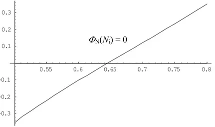
Under (18) we have xa = –0,822 and xi = –0,223 This implies that the agricultural sector’s learning by doing exhibits decreasing returns and the industrial sector increasing returns. As shown in the proposition, the system may have two equilibrium points. From the proposition we know that the variables, r, Ni, Na, La, la and li are determined, independent of the two variables H and Ki. This implies that when the system has two equilibrium points, the rate of interest, the labour distribution and land-use distribution are equal at the two points16_{. The}

variable Ni is determined by equation (A17), ΦN(Ni) = 0. Figure 1 shows that the equation has a unique solution.

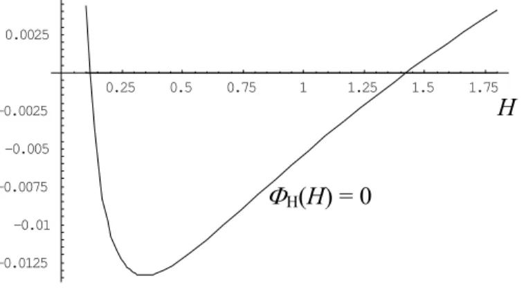
We uniquely determine r, Ni, Na, La, la and li as in Table 1. We see that most of the labour force is located in the city. The farmer’s lot size is much larger than the urban worker’s lot size The variable H is determined by equation (A20), ΦH(H) = 0. Figure 2 shows that the equation

0.55 0.6 0.65 0.7 0.75 0.8

-0.3 -0.2 -0.1 0.1 0.2 0.3

Figure 1. The unique labour distribution.

0.25 0.5 0.75 1 1.25 1.5 1.75

-0.0125 -0.01 -0.0075 -0.005 -0.0025 0.0025

Figure 2. The existence of two equilibrium points of human capital.

has two solutions: H1 = 0,115 and H2 = 1,427. We denote the two equilibrium points using subscripts 1 and 2. We call the two equilibrium points as advanced equilibrium (AE) and underdeveloped equilibrium (UE). Following the proposition, we determine the equilibrium values of the other variables, which are summarized as in Table 1.

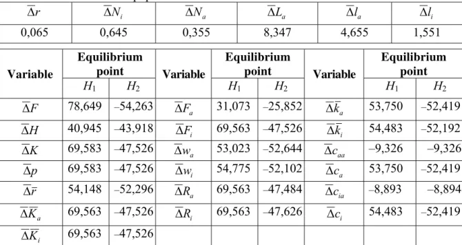
Table 1. The variables’ values at the two equilibrium points, H1 and H2.

r N_i N_a L_a l_a l_i

0,065 0,645 0,355 8,347 4,655 1,551

Equilibrium point

Equilibrium point

Equilibrium point Variable

H1 H2

Variable

H1 H2

Variable

H1 H2

F 0,211 8,504 F_a 0,504 2,388

a

k 0,161 3,946

H 0,115 1,427 F_i 0,174 4,280

i

k 0,223 5,473

K 1,001 24,761 w_a 0,071 1,743 c_aa 0,016 0,159

p _{0,072 1,769}

i

w 0,149 3,651 c_a 0,023 0,564

r 0,130 3,184 R_a 0,003 0,085 c_ia 0,021 0,221

a

K 0,188 4,623 R_i 0,014 0,353 c_i 0,016 0,391

i

K 0,820 20,138

We see that the difference in the levels of human capital at the two equilibrium points is very large. The level of the human capital at the AE is more than 12 times higher than that at the UE. The ratio between the national output levels, F (= Fi + p⋅Fa), is 42 times. The price of the agricultural goods, land rent, and the wage rate at the AE are all much higher than the corresponding variables at the UE. The output levels of the two sectors, the per capita wealth levels of the rural and urban residents, and the per capita consumption levels of the two products by the rural and urban residents at the AE are all much higher than the corresponding variables at the UE.

In the literature of economic development, it is well known that there may be multiple equilibrium points for the same type of economy when market imperfections or endogenous human capital are introduced into economic dynamics. This implies, for instance, that two seemingly identical regions may follow radically different development paths, one leading to

H

prosperity, the other to stagnation. Taiwan and Mainland China may provide a proper case for this result. Although they had similar backgrounds in terms of cultural heritage, values, and initial human capital, Taiwan and Mainland China had experienced totally different paths of industrialization during the period 1950-1980 – the former rapidly moved to the high equilibrium point, while the latter cycled around the low equilibrium point. It should be remarked that Canning [8] proposes a two-sector model with increasing returns to scale in the industrial sector and diminishing returns in agriculture. The model demonstrates that increasing demand for food coupled with diminishing returns in agriculture may not be a barrier to economic growth17. Canning’s model shows that the growth of the economy may be unlimited, despite ever increasing demand for agricultural procedure and in the absence of technical progress, if the increasing demands in the capital goods industry are sufficient to outweigh the diminishing returns to capital in agriculture. The equilibrium point with the higher level of human capital in our model explains what the Canning model predicts. It should be remarked that the concerns of classical economists, such as Ricardo, about capital accumulation with agriculture and industry can be explained by the case of the decreasing returns to scale in the two sectors.

CHANGES IN THE PRODUCTIVITY LEVEL, THE POPULATION, AND

THE PROPENSITY TO SAVE

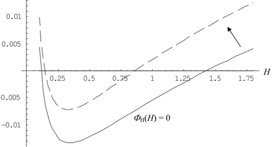
We now examine how the parameters affect the economic structure and labour distribution. First, we examine the case that all the parameters, except the productivity of the industrial sector Ai, are the same as in (18). We increase the productivity level Ai from 1,1 to 1,15. We introduce a symbol ∆ to stand for the change rate of the equilibrium value of a variable in percentage due to the change in a parameter value from. For instance, with regard to a variable xj, assuming the change of a parameter Ai from its current value Ai0 (which equals 1,1 in this case) to the new value Ai1 (equal to 1,15), we have

( )

( )

( )

0

1 − _×

≡ ∆

i j

i j i j j

A x

A x A x x

0.25 0.5 0.75 1 1.25 1.5 1.75

-0.01 -0.005 0.005 0.01

Figure 3. Shifts of the two equilibrium points as Ai rises.

Table 2. The effects as the industrial sector’s total productivity rises. Values of variables are given at two equilibrium points, H1 and H2.

Equilibrium point

Equilibrium point

Equilibrium point Variable

H1 H2

Variable

H1 H2

Variable

H1 H2

F

∆ 49,971 –50,099

a

F

∆ 17,724 –25,932

a

k

∆ 45,524 –42,932

H

∆ 26,020 –39,936

i

F

∆ 45,524 –42,932

i

k

∆ 45,524 –42,932

K

∆ 45,524 –42,932

a

w

∆ 45,524 –42,932

aa

c

∆ 0 0

p

∆ 45,524 –42,932

i

w

∆ 45,524 –42,932

a

c

∆ 45,524 –42,932

r

∆ 45,524 –42,932

a

R

∆ 45,524 –42,932

ia

c

∆ 0 0

a

K

∆ 45,524 –42,932

i

R

∆ 45,524 –42,932

i

c

∆ 45,524 –42,932

i

K

∆ 45,524 –42,932

We also analysed the case when Aa: 0,9 → 1. It can be shown that the variables r, Ni, Na, La, la and li are not affected and the two solutions of H are changed similarly to Figure 3. The change directions in the variables are the same as in Table 2, except that the per capita consumption levels of the farmers are affected but the consumption levels of the urban workers are not affected. As we increase τi: 0,05 → 0,055 the variables, r, Ni, Na, La, la and li are not affected and the two solutions of H are changed similarly to Figure 3. The change directions in the variables are the same as in Table 2. We now allow the population to rise as follows: N: 1,0 → 1,1. It is demonstrated that the two solutions of H are changed similarly to Figure 3. The level of human capital at UE is increased and the level at the AE is reduced. The changes in the equilibrium values of the variables are given in Table 3. As the total population rises, the rate of interest is not affected. The urban population rises by 9,6 % and the rural population rises by 10,8 %. The residential lot sizes in the rural and urban area fall respectively by 9,4 % and 8,7 %. The level of human capital at the UE rises by 41 % and the

H

the opposite effects upon the variables at the AE and the UE, except for the per capital levels of consumption of the agricultural goods which are reduced at the both equilibrium points. The equilibrium values at the UE are increased and the equilibrium values at the AE are reduced. A larger population benefits the long-term economic growth. As the population is increased, the UE is improved and the AE is lowered.

Table 3.The effects as the population rises.

r

∆ ∆N_i ∆N_a ∆L_a ∆l_a ∆l_i

0,065 0,645 0,355 8,347 4,655 1,551

Equilibrium point

Equilibrium point

Equilibrium point Variable

H1 H2

Variable

H1 H2

Variable

H1 H2

F

∆ 78,649 –54,263

a

F

∆ 31,073 –25,852

a

k

∆ 53,750 –52,419

H

∆ 40,945 –43,918

i

F

∆ 69,563 –47,526

i

k

∆ 54,483 –52,192

K

∆ 69,583 –47,526

a

w

∆ 53,023 –52,644

aa

c

∆ –9,326 –9,326

p

∆ 69,583 –47,526

i

w

∆ 54,775 –52,102

a

c

∆ 53,750 –52,419

r

∆ 54,148 –52,296

a

R

∆ 69,563 –47,484

ia

c

∆ –8,893 –8,894

a

K

∆ 69,563 –47,526

i

R

∆ 69,563 –47,626

i

c

∆ 54,483 –52,419

i

K

∆ 69,563 –47,526

An important issue in growth theory is related to interdependence between the propensity to save and national wealth. The study of individual thrift and national wealth has long been important in economics because national saving is the source of the supply of capital, a main factor of production affecting the productivity of labour. Thrift had traditionally been regarded as a virtuous, socially beneficial act. Admit Smith argued that capital is increased by parsimony and diminished by prodigality. He believed that parsimony, and not industry, is the immediate cause of the increase in capital. Smith said that prodigals are public enemies. This belief was strongly challenged by Keynes in the General Theory. He suggested that saving is potentially disruptive to the economy and harmful to social welfare. High propensity to save may reduce consumption, without systematically and automatically giving rise to an offsetting expansion in investment. This might thus cause demand to fall lower than proper level and hence output and employment lower than the capacity of the economy. We show that in economies with returns to scale the impact of the propensity to hold wealth are situation-dependent. An increase in the propensity to save may either increase or reduce the national wealth, depending on the current situations of the system. This implies that both Smith and Keynes are right under some situations and wrong under others.

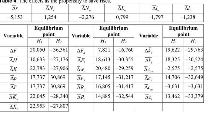
We increase the propensity to save as follows, λ0: 0,7 → 0,73. The two solutions of H are changed similarly to Figure 3. The changes in the equilibrium values of the variables are listed in Table 4. As the propensity to save rises, the rate of interest falls. The urban population rises and the rural population falls. The land for agricultural use is increased. The lot sizes in the urban and rural areas are reduced. The levels of human capital and national output are reduced at the AE and increased at the UE.

both equilibrium points. To see how caa and cia are reduced at the both equilibrium points, we note that as the propensity to save rises, the propensities to consume lot size, industrial goods, and agricultural goods fall relatively. The falls in the propensities tend to reduce the lot size, the consumption levels of the industrial agricultural goods and affect the prices of these goods. On the other hand, the changes in the incomes also affect the consumption levels of these variables and their prices. The net effects upon the consumption levels of the agricultural goods are negative at the both equilibrium points19_.

Table 4. The effects as the propensity to save rises.

r

∆ ∆N_i ∆N_a ∆L_a ∆l_a ∆l_i

–5,153 1,254 –2,276 0,799 –1,797 –1,238

Equilibrium point

Equilibrium point

Equilibrium point Variable

H1 H2

Variable

H1 H2

Variable

H1 H2

F

∆ 20,050 –36,361

a

F

∆ 7,821 –16,760

a

k

∆ 19,622 –29,763

H

∆ 10,633 –27,176

i

F

∆ 18,613 –30,355

i

k

∆ 18,325 –30,524

K

∆ 22,783 –27,906

a

w

∆ 20,480 –29,259

aa

c

∆ –2,575 –2,575

p

∆ 17,737 30,869

i

w

∆ 17,145 –31,217

a

c

∆ 14,706 –32,649

r

∆ 17,737 30,869

a

R

∆ 16,805 –31,417

ia

c

∆ –3,631 –3,631

a

K

∆ 22,045 –28,340

i

R

∆ 14,885 –32,544

i

c

∆ 13,462 –33,379

i

K

∆ 22,953 –27,807

CONCLUDING REMARKS

model in some directions. For instance, we may introduce some kind of government intervention in education into the model. It is also desirable to treat leisure time as an endogenous variable.

APPENDICES

A1: PROVING THE PROPOSITION

By equations (11) and (17) at equilibrium we have sj = k_j, j = a, i.

H NH F N NH F N h i i i a a a i a δ τ τ δ

δ + = . (A1)

From equations (2) and (4) we have

a i a i a i F K F K p α α

= (A2)

Substitute La = ς⋅p⋅Fa/Ra in (2) and lj⋅Rj = η⋅ŷj in (10) into the land constraints (16)

i i i

iN RL

yˆ =

η , ςpF_a +ηyˆ_aN_a =R_aL (A3)

Adding the two equations in (A3), we obtain

r =(ςpFa + ηŷiNi + ηŷaNa)/N. (A4)

From sj = kj in (A1) and sj = λ⋅ŷj we have ŷj = kj/λ. Substitute that and equation (A2) into

equation (A4) we obtain

r=(α0KaFi/Ki+ ηK/λa)/N. (A5)

where we used equation (13) and α0≡αiς/αa. Substitute p⋅cja = µ⋅ŷj in (10) into equation (14)

µ⋅K = λ⋅p⋅Fa. (A6)

Substituting equations (10) into equation (15) yields

δ0⋅K = Fi (A7)

where δ0≡ξ/λ + δk. Substituting equations (A2) and (A7) into equation (A6) yields

Ka = δλ⋅Ki, (A8)

where δλ≡µ⋅αa/αi(ξ+ δk⋅λ). From equations (A8) and (13), we have

K = (1 + δλ)Ki (A9)

Equations (A8) and (A9) determine Ka and K as unique functions of Ki. Substitute equations (A7) into (A9) into (A5)

i

K r

r = ₀ , (A10)

where

0

r = (1 + δλ)⋅(α0δλδ0+ η /λ)/N.

From equations (4), (A7) and (A9), we have

(

)

(

)

0 i i i i k i N K w

r =αδ +δ_λ −δ = βδ +δλ (A11)

From equations (2) and (A8), we obtain

. , a i a k a a i a k a N K r w K r pF _⎟⎟ ⎠ ⎞ ⎜⎜ ⎝ ⎛ + = ⎟⎟ ⎠ ⎞ ⎜⎜ ⎝ ⎛ + = α δ δ β δ α δ λ

λ (A12)

Inserting equations (10) into utility functions (8) and then applying equation (12), we obtain

in which we use ŷj = k_j/λ and equations (9). Substitute ŷj = k_j/λ and p⋅Fa in (A12) into equations (A3)

,

, _{2 3}

1 i i a i a a

i mk N R m K m k N

R = = + (A14)

where

. ,

, _{2 3}

1 L m L r m L m a k i λ η ςδ α δ λ η _λ ≡ ⎟⎟ ⎠ ⎞ ⎜⎜ ⎝ ⎛ + ≡ ≡

Insert equations (A14) into equation (A13)

. 3 2 1 a i d a a a d i i i a a i i i N k N k N k m K m N k m ρ ρ ρ ρ η θ θ = ⎟⎟ ⎠ ⎞ ⎜⎜ ⎝ ⎛

+ (A15)

From ŷj = kj/λ and equations (A10) and (6), we have wj + r K0 i = r1kj where r1 ≡ 1/λ – r.

Substituting equations (A8), (A11) and (A12) into the above equations, we have

(

)

k ≡ +

(

_{) (}

₎

(

)

(

)

0

5 m r r N

m

a a k

i + ≡ + +

≡ α δ β δ δ δ β λ λ

Substitute equations (A16) yields into equation (A15)

( )

(

₍

)

₎

₍

₎

0 6 0 5 1 1 0 6 3 2 1 0 5 1 = ⎟⎟ ⎠ ⎞ ⎜⎜ ⎝ ⎛ − + − − ⎟⎟ ⎠ ⎞ ⎜⎜ ⎝ ⎛ − + + ≡

Φ − ₋

i i d i a d i i i i i N N r m N r m N N N N r m m m r N r m m N a i ρ ρ ρ ρ η θ θ (A17)

where we use Na + Ni = N and equations (13) and (A9). This equation contains a single variable. The labour distribution is determined by a positive Ni such that

ΦN(Ni) = 0, 0 < Ni < N.

We require ρdj – 1 < 0, j = a, i. As ΦN(N) > 0 we see that the problem has at least one meaningful solution. As it is difficult to discuss conditions whether the problem has a unique solution, we will confirm whether the labour distribution is unique when simulating the model. From equation (A17) and Na = N – Ni we determine the labour distribution as a function of the population and other parameters.

For any given Ni from equations (3) and (4), we solve Ki as a function of H , / 0 i i m

i m H

K = β (A18)

in which . / 1 0 i k i i _N r A m i β δ α ⎟⎟ ⎠ ⎞ ⎜⎜ ⎝ ⎛ + ≡

From equations (A17) and (A11) we may consider m0 as a parameter. From equations (A16) we solve k_i and k_a as functions of H

, , , / i a j H q

k mi i

j

j = =

β (A19) where

(

)

q ≡ +

From equations (A14) and (A16), we get Ra = m4Ki, where m4≡m2 + (m6 – r N0 i)m3/r1. From

Ra = m4Ki and equations (2) and (A12), we obtain

a k a r m L α δ ςδ_λ + =

4

.

We now determine H. Substituting equations (1) and (3) into the last equation in (A1), we obtain the following equation

, 0 ) ( ) ( )

( ≡Φ +Φ − =

Φ_h H _a H _i H δ_h

(A20) where we use equations (A8) and (A18) and

. 1 , 1 , ) ( , ) ( 0 1 0 1 − − ≡ − − + ≡ ≡ Φ ≡

Φ + +

i i i i a a i i a a x i i i i x a a a a a m x m m x H N m N A H H N m L N A H i i i a a a a ε β ε β α τ δ

τ α α β α

λ ς β

We omit the case of xa = xi = 0. Equilibrium of the system is given by a positive H such that

Φ(H) = 0. When xa > 0 and xa > 0 equation Φ(H) = 0 has a unique positive solution as Φ’ = 0 for any positive H, Φ(H) < 0 and Φ(∞) > 0. Similarly, if xa < 0 and xi < 0 the equation

Φ(H) = 0 has a unique positive solution. It is easy to check that if either xa = 0, or xi = 0 then the system has a unique positive solution under certain conditions. We now prove that if

xa > 0and xi < 0 (or xa < 0 and xi > 0), then the system has either two solutions or no solution. It is sufficient for us to examine one case, for instance that with xa > 0 and xi < 0. Since

Φ(H) > 0, Φ(∞) > 0 we see that Φ(H) = 0 cannot have a unique solution. That is, the equation

Φ(H) = 0 has either multiple solutions, or no solution. On the other hand, as Φ’(H) = 0 has a unique positive solution, we conclude that Φ(H) = 0 has two solutions if Φ(H) has solutions. The necessary and sufficient condition for the existence of two solutions is that there exists a positive value H1 of H such that Φ(H1) < 0 and Φ’(H1) = 0. We have thus proved the proposition.

A2: DESCRIBING THE MOTION WITH THREE DIFFERENTIAL EQUATIONS

We now show a procedure to determine dynamic properties of the system. We omit time index in expressions in Appendix A2. Similar to equation (A4), we have

, ˆ ˆ / 0 N N y N y K F K

r = α a i i +η i i +η a a _(A21)

where we use equation (A2) and α0≡αiς/αa. Substitute p⋅cja = µ⋅ŷj in (10) into equation (14)

(

)

µ (A22)

Substituting equations (10) into equation (15) yields

(

)(

)

From equations (A22) and (A23), we have

.

µ λ ξ δ ₌ + + a i pF K F (A24)

Substituting equation (A2) into equation (A24) yields

(

)

(

)

= (A25)

From equation (A25) and K = Ka + Ki we solve

(

)

,

1 _{i i}

K F F K K αδ α − +

in which α ≡αaµ/αi

(

)

i(t) and H(t). We see that Ka(t) is also determined as a function of Ki(t) and H(t). Substitute equation (A21) into the definitions of ŷj in (6), we obtain

(

)

ˆ 0 _{j a i}

N N y N y K F K w k r

y a i i i i a a

j j j = + + + + +

= α η η (A27)

Solving previous equations, we obtain

(

)

(

)

y i i a i i a

i η η α − + + + +

= yˆ_a = k + yˆ_i, (A28)

in which k = (1 + r)(k_a– k_i) + wa – wi. From equations (4), we see that r and wi can be considered as functions of Ki, H and Ni. From equations (A3), we have

(

)

= (A29)

By equations (A2) and (A29), p and wa are also functions of Ki, H and Ni. Using Na = N – Ni and equations (A2) and (A29), we can express ŷi as a unique function of ka, ki, Ki, H and Ni:

(

)

k k k K H N

k = Ψ

(

)

ˆ_i k_i k_a K_i H N_i

y = Ψ (A30)

Inserting equations (10) into utility functions (8) and then applying equation (12), we obtain

, ˆ ˆ a i d a a a d i i i a i N y N y R R θ θ η = ⎟⎟ ⎠ ⎞ ⎜⎜ ⎝ ⎛ (A31)

in which we also use (9). Substitute equations (A3) into equation (A31)

, ˆ ˆ ˆ 1 0 a i d a a d i i a a i i a N y N y N y K F

K _η η _θ η η

α − − −

= ⎟⎟ ⎠ ⎞ ⎜⎜ ⎝ ⎛

+ (A32)

where we use (A2) and

. η η θ θ θ _⎟⎟ ⎠ ⎞ ⎜⎜ ⎝ ⎛ ≡ a i a i L L

Substitute equations (A28) into equation (A30)

(

)

(

)(

)

(

)(

)

, , , , 1 0 = − Ψ + Ψ Ψ − ⎟⎟ ⎠ ⎞ ⎜⎜ ⎝ ⎛ Ψ + Ψ − + ≡ Ψ − − − a i d i k d i k i i i a i i a i N N N N N K F K N H K k k η η η _θ η α (A33)

Assume that from equation (A33) we determine Ni as a function of ka, ki, Ki and H:

(

)

N_i ≡ Ψ_{N i a i} (A34)

From equation (A34) and Na = N – Ni, we determine the labour distribution as functions of

a

k , k_i, Ki and H. From equation (13) and Na = N – Ni we have

(

) (

)

N k K

K_a + _i = _a + _i − _a Ψ_{N i a i} (A35)

Equation (A35) contains four variables: k_a, k_i, Ki and H. Assume that we solve ka as a

function of k_i, Ki and H as follows

(

)

0 k K H

k_a = Ψ _{i i} (A36)

By the following procedure, we can determine all the variables as functions of k_i(t), Ki(t) and

by equation (A27) → wa by (A29) → ŷa by (A0) → li = Li/Ni → Ra by (A3) →la and Ri by equations (10) → ca, caa and sa by equations (10) → ci, cia and si by equations (10) → Fi by equation (3) →Fa by equation (1). From equations (11), (17) and (A36), we have

( )

( ) ( )

(

)

)

(t = Λ k t K t H t ≡ s t − Ψ₀

k&_{a a i i a} (A37)

( )

( ) ( )

(

)

)

(t k t K t H t s t k t

k&_i = Λ_{i i i} ≡ _i − _i

( )

(

( )

( ) ( )

)

( ) ( )

_{( )}

( ) ( )

_{( )}

( )

t NH

t F t N t

NH t F t N t

H t K t k t

H a a a i i i _h

i i

H _{a i} δ

τ τ

ε

ε + −

≡ Λ

=

& _(A38)

Taking derivatives of equation (13) with respect to t we obtain , 0 0

0 k K H

k&_a = Ψ_k&_i + Ψ _K &_i + Ψ _H & (A39)

where Ψ_0k, Ψ_0K and Ψ_0H are partial derivatives of Ψ₀ with respect to k_i(t) Ki(t) and H(t),

respectively. From equations (A37) and (A39), we delete k&_a and obtain

( )

(

( )

( ) ( )

)

0

0 0

K

i k H H a

i i K

i t k t K t H t

K

Ψ

Λ Ψ − Λ Ψ − Λ ≡ Λ

=

& _(A40)

Equations (A38) and (A40) contain three variables: k_i(t), Ki(t) and H(t). The three differential equations determine the motion of k_i(t), Ki(t) and H(t) over time. All other variables are determined as functions of the three variables at any point of time. As the expressions are tedious, t is difficult to interpret analytical results. We are concerned only with equilibrium issues.

ACKNOWLEDGMENT

The author is grateful to important comments of two anonymous referees.

REMARKS

The model was first presented in [9] and [10]. The original static model has been extended in different ways (see for instance, [10 – 12]). As mentioned by Fields [13], the model has been extended to allow for an urban informal sector, on-the-job search from agriculture, duality within the rural sector, educational differences among workers, job fixity, mobile capital, endogenous urban wage setting, risk-aversion, a system of demand of goods and many other factors. The list of extensions can be much longer.

2_{The assumption by Matsuyama is not supported by the empirical evidence presented in [14]}

and [15]. It is demonstrated that growth in total factor productivity in agriculture is not only strictly positive but, in most cases, larger than total factor productivity growth in industry. It should also be remarked that the two-sector model presented in [8] fixes the saving rate and does not consider endogenous change in human capital.

3_{The assumption of full utilization of factor resources is strict. However, as shown in [3] for a}

two-sector economy with constant human capital, it is conceptually not difficult to relax the assumption of full employment of labour force. Nevertheless, the model with unemployment and human capital will become difficult to analyze.

4

Although this assumption is often accepted in the literature of urbanization with agriculture (see [17, 18]), some studies try to examine impact of transportation costs upon urban-rural labour distribution (e.g., [19, 20]).

5_{As the urban land used for industrial sector is not large, the omission of industrial land use is}

6

Zhang has also examined the relations between his approach and the Solow growth theory, the Ramsey growth theory, the permanent income hypothesis, and the Keynesian consumption function in details.

7

The concept of amenity is often used in the literature of urban and regional economics (see, for instance, [6, 21 – 24]). The concept has recently been introduced into the Ramsey growth model in [25].

8_{The Keynesian consumption function and permanent income hypotheses (which are not the}

same) are similar to our approach in the sense that the propensity to save is affected by wealth. It should be noted that Zhang’s approach is very general in the sense that by introducing endogenous taste change, Zhang’s approach generates the same consumer behaviour as described by the traditional approaches (see [3]).

9_{Another important issue is about taste change. In any basic course in microeconomics,}

concepts of normal, inferior, and luxury goods are introduced. For illustration, we now point out possible ways to take account of a household’s preference change due to changes in income. Let there be n kinds of goods and services. The household’s utility function is given, for instance, by

∏

=

= n

j t j t

t c t s t

U j

1 ) ( )

(

) ( )

( )

( λ ξ ,

where cj(t) is the consumption level of goods j, s(t) is the saving, and the preference parameters are defined similarly as in (8). The budget constraint is given by

∑

=

= +

n

j

j

j t c t s t y t p

1

) ( ˆ ) ( ) ( ) (

where ŷ(t) is the disposable income. The optimal solution is

s(t) = λ(t)ŷ(t), cj(t) = ξj(t)ŷ(t)/pj(t), j = 1, …, n. Here, we consider that the propensities are influenced by the household’s disposable income

(and/or wage and wealth), his age, and other factors like relative social status in the following way:

λ(t) = λ[ŷ(t), t], ξj(t) = ξj[ŷ(t), t], j = 1, …, n. For instance, if good 1 is an inferior good, and the others are normal, we may specify the

preference change as follows: ξ1(t) = ξ10 – ξ11⋅ŷ(t), ξ1(t) > 0, where ξ10 and ξ11 are constants and the rest of the parameters are kept constant. The preference change may be nonlinear. We will not examine taste change in this study as the analysis is already very complicated.

10

In the contemporary literature of growth theory, different sources of human capital, such as education, are introduced to explain economic growth and development (see, e.g. [26 – 29]). This study is limited the case of learning by doing. It should be noted that Zhang [30] takes account of three sources of learning, learning by doing, learning by leisure, and learning by education.

11

For simplicity, we assume a linear relation between the outputs and growth rate of human capital. It is important to examine what will happen to the system if the growth rate is related to the outputs with some reasonable nonlinear relations.

12_{Although we failed to explicitly give stability conditions, Appendix A2 shows the}

procedure of finding out the dynamic equations of the economic system.

13_{As mentioned before, the main extension of this study is to introduce amenity differences}

14

This assumption is accepted, for instance in [5].

15_{The specification is strict. For instance, as the urban area is expanded, the city may become}

more attractive.

16_{These properties are mainly due to the specified forms of the utility and production}

functions.

17

The problem of increasing demand for food coupled with diminishing returns in agriculture was central to the classical growth theories of Malthus and Ricardo. In [10], Panagariya and Succar introduce economies of scale to the Harris-Todaro framework with fixed capital within a static framework.

18_{See [3] for more detailed discussions on multiple equilibrium points with different levels of}

human capital.

19_{We also demonstrate that the urban amenity parameter is improved, some people will}

migrate from the rural area to the urban area. The urban lot size falls and the rural lot size and agricultural land use are increased. The effects of the urban amenity improvement are similar to those caused by the productivity improvement.

REFERENCES

[1] Brueckner, J.K. and Zenou, Y.: Harris-Todaro Models with a Land Market.

Regional Science and Urban Economics 29, 317-239, 1999,

[2] Matsuyama, K.: Agricultural Productivity, Comparative Advantage, and Economic Growth.

Journal of Economic Theory 58: 317-334, 1992,

[3] Zhang, W.B.: Economic Growth Theory.

London, Ashgate, 2005,

[4] Harris, J.R. and Todaro, M.P.: Migration, Unemployment and Development: A Two-Sector Analysis.

American Economic Review 60, 126-142, 1970,

[5] Irz, X. and Roe, T.: Seeds of Growth? Agricultural Productivity and the Transitional Dynamics of the Ramsey Model.

European Review of Agricultural Economics 32, 143-165, 2005,

[6] Zhang, W.B.: Monetary Growth Theory: Money, Interest, Prices, Capital, Knowledge, and Economic Structure over Time and Space.

Routledge, London, 2009.

[7] Arrow, K.J.: The Economic Implications of Learning by Doing.

Review of Economic Studies 29, 155-173, 1962,

[8] Canning, D.: Increasing Returns in Industry and the Role of Agriculture in Growth.

Oxford Economic Papers 40, 463-476, 1988,

[9] Todaro, M.P.: A Model of Labour Migration and Urban Unemployment in Less Developed Countries.

American Economic Review 59, 138-148, 1969,

[10] Panagariya, A. and Succar, P.: The Harris-Todaro Model and Economies of Scale.

Southern Economic Journal 52, 984-998, 1986,

[11] Shapiro, C. and Stiglitz, J.: Equilibrium Unemployment as a Worker Discipline Device.

American Economic Review 74, 433-444, 1984,

[12] Bencivenga, V.R. and Smith, B.D.: Unemployment, Migration, and Growth.

[13] Fields, G.S.: A Welfare Economic Analysis of Labour Market Policies in the Harris-Todaro Model.

Journal of Development Economics 76, 127-46, 2005,

[14] Bernard, A.B. and Jones, C.I.: Comparing Apples to Oranges: Productivity Convergence and Measurement Across Industries and Countries.

American Economic Review 86, 1216-1252, 1996,

[15] Martin, W. and Mitra, D.: Productivity Growth and Convergence in Agriculture Versus Manufacturing.

Economic Development and Cultural Change 49, 403-422, 2001,

[16] Mundlak, Y.: Agriculture and Economic Growth.

Cambridge, Harvard University Press, Ch. 8, 2000,

[17] Krugman, P.R.: Increasing Returns and Economic Geography. Journal of Political Economy 99, 483-499, 1991,

[18] Fujita, M. and Thisse, J.F.: Economics of Agglomeration.

Cambridge, Cambridge University Press, 2002,

[19] Fujita, M., Krugman, P.R. and Venables, A.J.: The Spatial Economy: Cities, Regions and International Trade.

Cambridge, MIT Press, 1999,

[20] Picard, P.M. and Zeng, D.Z.: Agriculture Sector and Industrial Agglomeration.

Journal of Development Economics 77, 75-106, 2005,

[21] Kanemoto, Y.: Theories of Urban Externalities.

Amsterdam, North-Holland, 1980,

[22] Diamond, D.B. and Tolley, G.S., eds.: The Economics of Urban Amenities.

New York, Academic Press, 1981,

[23] Blomquist, G.C.; Berger, M.C. and Hoehn, J.C.: New Estimates of Quality of Life in Urban Areas.

American Economic Review 78, 89–107, 1988,

[24] Andersson, Å.E.; Johansson, B. and Anderson, W.P., eds.: The Economics of Disappearing Distance.

Aldershot, Hampshire. Ashgate, 2003,

[25] Gerlagh, R. and Keyzer, M.A.: Path-Dependent in a Ramsey Model with Resource Amenities and Limited Regeneration.

Journal of Economic Dynamics & Control 28, 1159–1184, 2004,

[26] Lucas, R.E.: On the Mechanics of Economic Development.

Journal of Monetary Economics 22, 3-42, 1986,

[27] Romer, P.M.: Increasing Returns and Long-Run Growth.

Journal of Political Economy 94, 1002-1037, 1986,

[28] Barro, R.J. and Sala-i-Martin, X.: Economic Growth.

New York, McGraw-Hill, 1995,

[29] Grossman, G.M. and Helpman, E.: Innovation and Growth in the Global Economy.

Cambridge, MIT Press, 1991,

[30] Zhang, W.B.: Economic Growth with Learning by Producing, Learning by Education, and Learning by Consuming.

MODEL RASTA DVA SEKTORA S ENDOGENIM

LJUDSKIM RESURSIMA I MOGU

Ć

NOSTIMA

W.-B. Zhang

Azijsko pacifičko sveučilište Ritsumeikan prefektura Oita, Japan

SAŽETAK

Rad razmatra pitanja vezana uz urbanizaciju s migracijom radne snage. Glavna odstupanja od tradicionalnih pristupa dinamici ekonomskih struktura su što se u radu koristi alternativni pristup ponašanju potrošača te što se uvodi akumulacija ljudskog kapitala putem učenja stečenog djelovanjem. Model opisuje dinamičko međudjelovanje između poljoprivredne i industrijske proizvodnje, ruralne i urbane mogućnosti, distribuciju faktora proizvodnje i preferencija kao i akumulaciju endogenog kapitala i ljudskih resursa. Pokazujemo kako dinamički sustav može imati ili jedno, ili više ravnotežnih stanja, ovisno o povratku na skalu u dva sektora. Također smo ispitali učinke promjena pojedinih parametara modela.

KLJUČNE RIJEČI