The XWS open access catalogue of extreme European windstorms from 1979–2012

(1)

NHESSD

2, 2011–2048, 2014

The XWS catalogue

J. F. Roberts et al.

Title Page

Abstract Introduction

Conclusions References

Tables Figures

◭ ◮

Back Close

Full Screen / Esc

Printer-friendly Version Interactive Discussion

Discussion

P

a

per

|

D

iscussion

P

a

per

|

Discussion

P

a

per

|

Discuss

ion

P

a

per

|

Nat. Hazards Earth Syst. Sci. Discuss., 2, 2011–2048, 2014 www.nat-hazards-earth-syst-sci-discuss.net/2/2011/2014/ doi:10.5194/nhessd-2-2011-2014

Natural Hazards and Earth System Sciences

Open Access

Discussions

This discussion paper is/has been under review for the journal Natural Hazards and Earth System Sciences (NHESS). Please refer to the corresponding final paper in NHESS if available.

The XWS open access catalogue of

extreme European windstorms from

1979–2012

J. F. Roberts1, A. J. Champion2, L. C. Dawkins3, K. I. Hodges4, L. C. Shaffrey5, D. B. Stephenson3, M. A. Stringer2, H. E. Thornton1, and B. D. Youngman3

1

Met Office Hadley Centre, Exeter, UK

2

Department of Meteorology, University of Reading, Reading, UK

3

College of Engineering, Mathematics and Physical Sciences, University of Exeter, Exeter, UK

4

National Centre for Earth Observation, University of Reading, Reading, UK

5

National Centre for Atmospheric Science, University of Reading, Reading, UK

Received: 13 January 2014 – Accepted: 12 February 2014 – Published: 7 March 2014

Correspondence to: J. F. Roberts ([email protected])

Published by Copernicus Publications on behalf of the European Geosciences Union.

(2)

NHESSD

2, 2011–2048, 2014

Title Page

Tables Figures

◭ ◮

Back Close

Full Screen / Esc

Discussion

P

a

per

|

D

iscussion

P

a

per

|

Discussion

P

a

per

|

Discuss

ion

P

a

per

|

Abstract

The XWS (eXtreme WindStorms) catalogue consists of storm tracks and model-generated maximum three-second wind-gust footprints for 50 of the most extreme winter windstorms to hit Europe over 1979–2012. The catalogue is intended to be a valuable resource for both academia and industries such as (re)insurance, for

ex-5

ample allowing users to characterise extreme European storms, and validate climate and catastrophe models. Several storm severity indices were investigated to find which could best represent a list of known high loss (severe) storms. The best performing

index wasS_ft, which is a combination of storm area calculated from the storm footprint

and maximum 925 hPa wind speed from the storm track. All the listed severe storms are

10

included in the catalogue, and the remaining ones were selected usingS_ft. A

compari-son of the model footprint to station observations revealed that storms were generally well represented, although for some storms the highest gusts were underestimated due to the model not simulating strong enough pressure gradients. A new recalibra-tion method was developed to estimate the true distriburecalibra-tion of gusts at each grid point

15

and correct for this underestimation. The recalibration model allows for storm-to-storm

variation which is essential given that di_fferent storms have di_fferent degrees of model

bias. The catalogue is available at www.europeanwindstorms.org.

1 Introduction

European windstorms are extra-tropical cyclones with very strong winds or violent

20

gusts that are capable of producing devastating socioeconomic impacts. They can lead to structural damage, power outages to millions of people, and closed transport net-works, resulting in severe disruption and even loss of lives. For example the windstorms Anatol, Lothar and Martin that struck in December 1999 inflicted approximately 13.5 Billion USD (indexed to 2012) worth of damage, and lead to over 150 fatalities (Sigma,

25

(3)

NHESSD

2, 2011–2048, 2014

Title Page

Tables Figures

◭ ◮

Back Close

Full Screen / Esc

Discussion

P

a

per

|

D

iscussion

P

a

per

|

Discussion

P

a

per

|

Discuss

ion

P

a

per

|

By cataloguing these events, the intensity, location and frequency of historical wind-storms can be studied. This is crucial to understanding the factors that influence their development (such as the North Atlantic jet stream or the North Atlantic Oscillation), and for evaluating and improving the predictions of weather and climate models.

Publically available historical storm catalogues, such as HURDAT (Landsea et al.,

5

2004) and IBTRACS (Levinson et al., 2010), are widely used in the tropical cyclone community. These catalogues provide quantitative information about historical tropical cyclones, including observed tracks of storm position and intensity. Tropical cyclone catalogues are an essential resource for the scientific community and are used to un-derstand how climate variability modulates the development and activity of tropical

10

cyclones (e.g., Ventrice et al., 2012) and for evaluating climate models (e.g., Strachan et al., 2013; Manganello et al., 2012). These catalogues are also widely used within the insurance and reinsurance industry to assess risks associated with intense tropical cyclones.

Despite the utility of tropical cyclone catalogues, no comparable catalogue of

Euro-15

pean windstorms currently exists. One of the last major freely available catalogues was that of Lamb (1991). This catalogue has not been digitised and is now long out-of-date. More recent catalogues only contain information on storm intensity (Della-Marta et al., 2009), only pertain to a specific country (e.g., Bessemoulin, 2002), or are not publically available. The XWS catalogue, available at www.europeanwindstorms.org, aims to

ad-20

dress this gap, by producing a publically available catalogue of the 50 most extreme European winter windstorms. The catalogue consists of tracks and model-generated maps of maximum three-second wind-gusts at each model grid point over a 72 h

pe-riod for each storm (hereafter the maps are referred to as the storm footprints, and

three-second wind-gusts as gusts).

25

In order to create the catalogue, several scientific questions had to be addressed:

1. What is the best method for defining extreme European windstorms?

(4)

NHESSD

2, 2011–2048, 2014

Title Page

Tables Figures

◭ ◮

Back Close

Full Screen / Esc

Discussion

P

a

per

|

D

iscussion

P

a

per

|

Discussion

P

a

per

|

Discuss

ion

P

a

per

|

2. How well do the model storm footprints compare with observations, and what are the reasons for any biases?

3. What is the best way to recalibrate the footprints given the observations?

This paper describes how the above questions were addressed to produce the XWS catalogue. The paper is structured as follows: Sect. 2 describes the data and methods

5

used to generate the storm tracks and footprints, and Sect. 3 describes the method used to select the 50 most extreme storms. Section 4 evaluates the storm footprints using weather station data, and Sect. 5 describes the recalibration method. Conclu-sions and future research directions are discussed in Sect. 6.

2 Data

10

This section describes the datasets and models used to produce the data for the 50 extreme European windstorms in the XWS catalogue, which consists of:

– Tracks of the 3 hourly locations of the maximum T42 850 hPa relative vorticity,

min-imum mean sea level pressures (MSLP) and maxmin-imum 925 hPa wind speed from the ERA Interim reanalysis identified by an automated cyclone tracking algorithm

15

(Hodges, 1995, 1999).

– Maximum three-second gust footprints over a 72 h-period using the ERA Interim

reanalysis dynamically downscaled using the Met O_ffice Unified Model.

– Recalibrated maximum three-second gust footprints using Met Office Integrated

Data Archive System (MIDAS) weather station observations.

20

(5)

NHESSD

2, 2011–2048, 2014

Title Page

Tables Figures

◭ ◮

Back Close

Full Screen / Esc

Discussion

P

a

per

|

D

iscussion

P

a

per

|

Discussion

P

a

per

|

Discuss

ion

P

a

per

|

2.1 Storm tracks

Storms are tracked in the European Centre for Medium Range Weather Forecasts (ECMWF) Interim Reanalysis (ERA Interim) data set (Dee et al., 2011), over 33 ex-tended winters (October–March 1979/80–2011/12). The identification and tracking of the cyclones is performed following the approach used in Hoskins and Hodges (2002)

5

based on the Hodges (1995, 1999) tracking algorithm. This uses 850 hPa relative vor-ticity to identify and track the cyclones.

Previous studies (Hodges et al., 2011) have used 6 hourly reanalysis data, but here 3 hourly data are used to produce more reliable tracks since some extreme European windstorms have very fast propagation speeds. The 3 hourly data are obtained for ERA

10

Interim by splicing the 3 h forecasts in between the 6 hourly analyses. Before the iden-tification and tracking progresses the data are smoothed to T42 and the large scale background removed as described in Hoskins and Hodges (2002), reducing the inher-ent noisiness of the vorticity and making tracking more reliable. The cyclones are idinher-enti- identi-fied by determining the vorticity maxima by steepest ascent maximisation in the filtered

15

data as described in Hodges (1995). These are linked together, initially using a nearest neighbour search, and then refined by minimizing a cost function for track smoothness (Hodges, 1995) subject to adaptive constraints on the displacement distance and track smoothness (Hodges, 1999). These constraints have been modified from those used for 6 hourly data to be suitable for the 3 hourly data. Storms that last longer than 2 days

20

are retained for further analysis. The algorithm identified 5730 storms over the 33 yr

period in a European domain defined as 15◦W to 25◦E in longitude, 35◦N to 70◦N in

latitude. 50 of these storms were selected for the catalogue as described in Sect. 3. The MSLP and maximum 925 hPa wind speed associated with the vorticity maxima are found in post-processing. This is done by searching for a minimum/maximum within

25

a certain radius of the vorticity maximum. A radius of 6◦ is used for the MSLP. For the

925 hPa wind speed, radii of 3◦, 6◦ and 10◦ were tested but only the results for 3◦ are

given as this was found to be the best indicator of storm severity (see Sect. 3.1). For

(6)

NHESSD

2, 2011–2048, 2014

Title Page

Tables Figures

◭ ◮

Back Close

Full Screen / Esc

Discussion

P

a

per

|

D

iscussion

P

a

per

|

Discussion

P

a

per

|

Discuss

ion

P

a

per

|

the MSLP the location of the minimum is only given if it is a true minimum. If not, the MSLP value given is that at the vorticity centre.

2.2 Windstorm footprints

2.2.1 Dynamical downscaling

The dataset used to create the windstorm footprints is generated by dynamically

down-5

scaling ERA Interim (T255 ∼0.7◦) to a horizontal resolution of 0.22◦ (equivalent to

∼24 km at the model’s equator). The atmospheric model used to perform the

down-scaling is the Met O_ffice Unified Model (MetUM) version 7.4 (Davies et al., 2005).

The model’s non-hydrostatic dynamical equations are solved using semi-Langrangian advection and semi-implicit time stepping. There are 70 (irregularly spaced) vertical

10

levels, with the model top being 80 km.

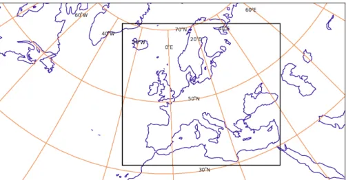
The downscaled region covers western Europe and the eastern North Atlantic

(here-after referred to as the “WEuro” region), and is shown in Fig. 1. The 0.22◦ MetUM grid

uses a rotated pole at a longitude of 177.5◦ and latitude 37.5◦ so that the grid spacing

does not vary substantially over the domain1. To drive the 0.22◦MetUM, lateral

bound-15

ary and initial conditions for the WEuro domain are generated from the ERA Interim

6 hourly analyses. The 0.22◦MetUM is initialised each day using the 18Z reconfigured

ERA Interim analyses and a 30 h forecast is performed. The first six hours are disre-garded due to spin up, allowing the model to adjust from the ECMWF IFS (the EMCWF Integrated Forecast System, ECMWF, 2006) initial conditions. This results in daily 24 h

20

forecasts for the full period. By combining the daily forecasts a new, higher resolution data set is created.

1

(7)

NHESSD

2, 2011–2048, 2014

Title Page

Tables Figures

◭ ◮

Back Close

Full Screen / Esc

Discussion

P

a

per

|

D

iscussion

P

a

per

|

Discussion

P

a

per

|

Discuss

ion

P

a

per

|

2.2.2 Creating the windstorm footprints

For this catalogue the footprint of a windstorm is defined as the maximum three-second gust at each grid point over a 72 h period during which the storm passes through the do-main. The three-second gust has been shown to have a robust relationship with storm damage (Klawa and Ulbrich, 2003), and is commonly used in catastrophe models

cur-5

rently used by the insurance industry. The 72 h period was chosen because again it is commonly used in the insurance industry (Haylock, 2011), and although lifetimes of windstorm can be longer than 72 h it is rare that the damaging winds associated with a windstorm last longer than this.

Maximum three-second gusts at a height of 10 m, which output every 6 h and give the

10

maximum gust achieved over the preceding 6 h period, from the 0.22◦MetUM dataset

are used to create the footprints. In the MetUM the gusts,U_gust, are estimated by finding

the value at which the normalised maximum gust, (U_gust−U_{10 m})/σ (whereU_{10 m}is the

10 m wind speed andσ is the standard deviation of the horizontal wind), has a 25 %

exceedance probability, i.e. P((U_gust−U_{10 m})/σ)> C)=0.25, giving U_gust=U_{10 m}+Cσ

15

(Beljaars, 1987). Cis estimated from the universal turbulence spectra, and σ is

esti-mated from the friction velocity using the similarity relation of Panofsky et al. (1977). Footprints were created for each of the 5730 storms identified by the tracking algo-rithm applied to ERA Interim (1979–2012; see Sect. 2.1). The 72 h period over which the maximum gusts were taken was centred on the time which the tracking algorithm

20

identified as having the maximum 925 hPa wind speed over land2within a 3◦ radius of

the track centre. This was done to ensure that the 72 h period of the footprint captured the storm at its most damaging phase.

2

Land on the ERA Interim grid in the European domain defined by 15◦W to 25◦E and 35◦N to 70◦N, excluding Iceland.

(8)

NHESSD

2, 2011–2048, 2014

Title Page

Tables Figures

◭ ◮

Back Close

Full Screen / Esc

Discussion

P

a

per

|

D

iscussion

P

a

per

|

Discussion

P

a

per

|

Discuss

ion

P

a

per

|

2.2.3 Footprint contamination

The European extratropical cyclones identified by the tracking algorithm are relatively frequent events. Over the 33 extended winters that have been tracked, on average 2.5 events pass through the domain in any given 72 h period. Furthermore, extra-tropical cyclones exhibit temporal clustering (Mailier et al., 2006), which could result in days

5

with even more storms. The highest number of storms passing through in a single 72 h period is 8, for the period starting at 00Z on 6 February 1985.

Footprints are therefore likely to include gusts from two or more windstorms. This can create problems when trying to attribute damage to a particular windstorm. To attempt to isolate the footprint to a particular windstorm, all the gusts within a 1000 km

10

radius3 of the track position at each 6 h timestep are assumed to be associated with

that particular windstorm and all other data is rejected. The “decontaminated” footprint is then derived by taking the maximum of these gusts within the 72 h period of the windstorm.

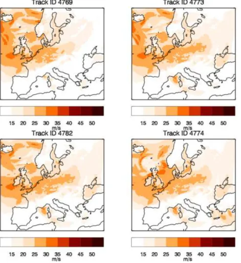
Figure 2 shows the footprints for windstorms with track IDs 4769, 4773, 4782, 4774,

15

centred on times 15Z 17 January 2007, 06Z 18 January 2007, 15Z 18 January 2007 and 18Z 19 January 2007 respectively, derived by taking maximum gusts over the whole domain (the contaminated footprints). The footprints are almost indistinguish-able, and are dominated by one large event. Figure 3 shows the footprints for the same windstorms, but created using the decontamination method described above. The new

20

footprints show that storm 4769 was in fact a very weak event over southern France and the Mediterranean Sea, storms 4773 and 4774 are northern storms which did not make much impact on land, and the dominant event is storm 4782, centred on 15Z 18 January 2007, which is the famous storm Kyrill (January 2007).

3

(9)

NHESSD

2, 2011–2048, 2014

Title Page

Tables Figures

◭ ◮

Back Close

Full Screen / Esc

Discussion

P

a

per

|

D

iscussion

P

a

per

|

Discussion

P

a

per

|

Discuss

ion

P

a

per

|

The uncontaminated footprints are used for the calculation of the storm severity in-dices (see Sect. 3), although in the catalogue both the contaminated and uncontami-nated footprints are available.

3 How to select extreme windstorms

Fifty of the most extreme storms of the 5730 identified by the tracking algorithm

5

(Sect. 2.1) have been selected for the XWS catalogue. The challenge when select-ing these storms was definselect-ing an “extreme storm”. A storm can be defined as extreme in many ways, for example in terms of a meteorological index, or extreme values of in-sured losses i.e. a severe event (Stephenson, 2008). Note that here severity is defined in terms of total insurance loss, however other measures are possible such as

hu-10

man mortality, ecosystem damage, etc. The aim here was to find an optimal objective meteorological index that selects storms that were both meteorologically extreme and severe. Expert elicitation with individuals in the insurance industry led to the identifica-tion of 23 severe storms in the period 1979–2012 (Table 1) which would be expected to be included if considering insured loss only. The most successful meteorological index

15

is considered to be the one that ranks most of these 23 severe as extreme (defined as category C storms in Sect. 3.2, Fig. 4a).

3.1 Possible meteorological indices

Meteorological indices from both the track and footprint of the storm were investigated.

These indices included the maximum intensity of the storm (Umax), defined as the

max-20

imum 925 hPa wind speed over continental European and Scandinavian land within

a 3◦radius of the cyclone track. Radii of 6◦and 10◦were considered, both resulting in

a slightly poorer performance by the index (fewer storms in category C). The size of the

storm (N) was also considered, defined as the area of the (uncontaminated) footprint

that exceeds 25 m s−1over continental European and Scandinavian land. A threshold

25

(10)

NHESSD

2, 2011–2048, 2014

Title Page

Tables Figures

◭ ◮

Back Close

Full Screen / Esc

Discussion

P

a

per

|

D

iscussion

P

a

per

|

Discussion

P

a

per

|

Discuss

ion

P

a

per

|

of 25 m s−1 was used as it is recognised as being the wind speed at which damage

starts to occur. In Lamb (1991) it was noted that wind speeds of 38–44 knots (19.5–

22.6 m s−1) damage chimney pots and branches of trees and wind speeds of 45–52

knots (23.1–26.8 m s−1) uproot trees and cause severe damage to buildings.

IndicesU_maxandN can be combined to form a storm severity index (SSI). Numerous

5

SSIs have been developed with their uses ranging from the estimation of the return period of windstorms over Europe (Della-Marta et al., 2009) to understanding how windstorms will change under anthropogenic climate change (Leckebusch et al., 2008). An SSI was used to rank the storms in the catalogue of extreme storms over the North Sea, British Isles and Northwest Europe by Lamb (1991). The SSI used by Lamb (1991)

10

is based on the greatest observed wind speed over land (V_max), the area affected by

damaging winds (A) and the overall duration of occurrence of damaging winds (D).

Damaging winds were defined as those in excess of 50 knots (25.7 m s−1):

S_Lamb=V_max3 AD.

The cube of the wind speed is a measure of the advection of kinetic energy and is used

15

to model wind power and damage (Lamb, 1991, p. 7). A similar SSI can be derived by

combining the track indexUmax3 (intensity) and footprint indexN (area) and assuming

that the duration of all storms is 72 h in accordance with the insurance industry defini-tion of an event (Haylock, 2011):

S_ft=U_max3 N.

20

Alternatively the intensity of a storm can be approximated from the footprint rather than the track, as the mean of the excess gust speed cubed at grid points over

Eu-ropean and Scandinavian land. Combining with indexN, this gives an SSI calculated

from the footprint only:

S_f= 

 1

N

X

land,ui>25

(u_i−25)3 

N=

X

land,ui>25

(u_i−25)3,

(11)

NHESSD

2, 2011–2048, 2014

Title Page

Tables Figures

◭ ◮

Back Close

Full Screen / Esc

Discussion

P

a

per

|

D

iscussion

P

a

per

|

Discussion

P

a

per

|

Discuss

ion

P

a

per

|

where ui is the maximum gust at grid point i in the footprint. A relative local 98th

percentile threshold can be used as an alternative to the fixed threshold, as in Klawa and Ulbrich (2003). This threshold implies that at any location storm damages are assumed to occur on 2 % of all days. This adaptation to wind climate can also be

expected to a_ffect the degree to which damage increases with growing wind speed in

5

excess of the threshold value, hence the normalised rather than absolute winds are used. In Klawa and Ulbrich (2003) weather station data are used, but an equivalent SSI can be calculated from the footprint to quantify the advantage of using a relative threshold when predicting severity:

S_f98= X land,u_i>u_98,_i

_u

i u_98,i

−1 3

, (1)

10

whereu_98,i is the 98 % quantile of maximum gust speeds during the reference period

(October–March, 1979–2012) at grid pointi. In Klawa and Ulbrich (2003) the summand

in Eq. (1) is multiplied by population density to calculate a loss index, but here the aim is to find a purely meteorological index for storm severity.

3.2 Results

15

The indices presented in Fig. 5 are related to one another. A positive association exists

betweenU_max and N and betweenS_ft and S_f98.S_ft has a stronger dependence on N

thanU_max and the strongest extremal dependence exists between S_ft and N. The 23

most severe storms are in the top 18 %, 7 %, 5 %, 10 % and 16 % of storms when

ranked according toU_max, N,S_ft,S_f (not shown) andS_f98 respectively, hence severe

20

storms are best characterised by a high value ofS_ft(Fig. 5e–h).

The catalogue will comprise of the 23 severe storms and 27 storms which are ex-treme in the optimal meteorological index. The intercept of the number of the 23 severe

storms in the top K storms andy=x−27 identifies the number of storms in category

C such that 50 storms are selected for the catalogue (Fig. 4b). U_max, N, S_ft, S_f and

25

(12)

NHESSD

2, 2011–2048, 2014

Title Page

Tables Figures

◭ ◮

Back Close

Full Screen / Esc

Discussion

P

a

per

|

D

iscussion

P

a

per

|

Discussion

P

a

per

|

Discuss

ion

P

a

per

|

Sf98 give 15, 15, 17, 10 and 13 storms in category C respectively (Table 2). The use

of the relative threshold indexS_f98 results in more storms in category C than the fixed

threshold equivalent,S_f. The index S_ft, however, maximises the number of storms in

category C and therefore is the most successful index at identifying both meteorologi-cally extreme and severe storms.

5

The location of the 50 storms selected by U_max,N and S_ft are broadly similar,

con-centrated around the UK and Northern Europe (Fig. 6a–c). These are Atlantic storms

which are strong and well represented in the reanalysis data. IndicesS_f andS_f98

se-lect very similarly located storms (Fig. 6d). They both sese-lect “meteorologically extreme and not severe” (category B) storms that are located in the Mediterranean which are

10

generally weaker and less well represented by the reanalysis data due to their small

scale (Cavicchia et al., 2013). Of the 27 category B storms selected byS_ft, 10 are also

selected byU_max, 9 byN and 4 by bothU_maxandN, demonstrating thatS_ftselects an

almost even combination of large area and intense wind speed storms.

IndicesU_max,N,S_ft,S_f (not shown) andS_f98select events from 29, 26, 27, 30 and

15

30 yr out of the 33 yr period 1979–2012 respectively, hence all indices represent the period spanned by the XWS catalogue well (Fig. 7). A similar trend exists within the time series for all 5 indices, with more storms selected in the period 1985–1995 and fewer in the period 2000–2010 (Fig. 7).

In summary the indexS_ft is the most successful index at identifying severe storms.

20

It depends on both the area and maximum wind speed intensity of the storm. The

indexS_ftselects storms located over the UK and Northern Europe and samples storms

over the full time period of the XWS catalogue, hence giving a good representation of the meteorologically extreme and severe Atlantic storms that occurred throughout the

period. For these reasonsS_ftis the meteorological index used to select the 50 storms

25

(13)

NHESSD

2, 2011–2048, 2014

Title Page

Tables Figures

◭ ◮

Back Close

Full Screen / Esc

Discussion

P

a

per

|

D

iscussion

P

a

per

|

Discussion

P

a

per

|

Discuss

ion

P

a

per

|

4 Evaluation of MetUM windstorm footprints

Observational data were extracted from the MIDAS database. For each of the selected storms, all stations roughly within the WEuro domain which recorded maximum gusts during the 72 h period were used to evaluate the MetUM windstorm footprints. The gust data were a mixture of 1, 3 and 6 hourly maximum gusts.

5

Example observational footprints for the storms Jeanette (October 2002) and Kyrill (January 2007) are shown in Fig. 8a and d. The observational footprints are defined in the same way as the model footprints, plotting the maximum gust over the same 72 h period, but instead of a gridded map they show the maximum gust recorded at the locations of each station. A quick inspection of the footprints shows that the model

10

and observations agree on the on the regions where the high gusts occur, although

it is difficult to confirm the exact affected region given the irregular locations of the

observations.

Figure 8c and f shows scatter plots of model maximum gusts against observed max-imum gusts for all of the stations in the observational footprint for each storm. The

15

MetUM maximum gusts for each specific station location were calculated using bilinear interpolation between grid points.

The scatter plots show that the gusts are scattered about they=xline, meaning that

in general the model gusts are in agreement with the observations. This result is espe-cially impressive when considering that the model gusts have simply been interpolated

20

from a∼25 km grid to a specific location without applying any corrections. For the 50

storms in the catalogue, the mean root mean square (RMS) error in the model gusts

is 5.7 m s−1(for stations at altitudes less than 500 m, and removing gusts for which the

observations read 0 m s−1which are believed to be erroneous).

However, two problems with the model are apparent from these scatter plots:

25

– For all storms there is a more dispersed population separate from the general

population, below the y=x line. It was found that these points are mostly from

stations with altitudes greater than∼500 m (plotted in red).

(14)

NHESSD

2, 2011–2048, 2014

Title Page

Tables Figures

◭ ◮

Back Close

Full Screen / Esc

Discussion

P

a

per

|

D

iscussion

P

a

per

|

Discussion

P

a

per

|

Discuss

ion

P

a

per

|

– For a number of storms the plots of model vs. observed gusts appears to

de-viate from the y=x line, flattening o_fffor observed gust speeds of greater than

∼25 m s−1, showing that the model is underpredicting extreme gusts. In Fig. 8

this can be seen for the storm Kyrill, although the problem is not so severe for the storm Jeanette.

5

The first issue has been noted previously, and is a common issue with climate and numerical weather prediction models (e.g. Donat et al., 2010; Howard and Clark, 2007).

It is caused by the use of an e_ffective roughness parametrisation, which is needed to

estimate the e_ffect of sub-grid scale orography on the synoptic scale flow, however it

causes unrealistically slow wind (and hence gust) speeds at 10 m.

10

In Howard and Clark (2007) a method was proposed to correct for this e_ffect, by

estimating a reference height,h_ref, above which the wind speeds are una_ffected by the

surface, and then assuming a log-profile to interpolate wind speeds back down to 10 m,

using the local vegetative roughness,z₀, rather than the e_ffective roughness.

In this model only wind speeds on seven model levels were archived which means

15

the estimation of wind speeds ath_ref could be subject to large errors. Nevertheless,

applying the correction to the storm Kyrill gave a clear improvement to the maximum 10 m winds for high altitude locations, although the underestimation of extreme gust

at lower altitudes remained (plot not shown). For this calculation h_ref was estimated

from orographic data at the resolution of the MetUM, but it is possible to estimatehref

20

from finer resolution data (as was done in Howard and Clark, 2007), which may further improve the correction.

It would be desirable to apply this correction to all of the storms in the catalogue, although the extraction of the archived data on all model levels is a time consuming and costly process and cannot be done at present. Instead, altitude is used as a covariate

25

(15)

NHESSD

2, 2011–2048, 2014

Title Page

Tables Figures

◭ ◮

Back Close

Full Screen / Esc

Discussion

P

a

per

|

D

iscussion

P

a

per

|

Discussion

P

a

per

|

Discuss

ion

P

a

per

|

4.1 Underprediction of high gusts for low altitude stations

Possible reasons for the underprediction of high gusts for low altitude stations de-scribed above include (i) the gust parameterisation scheme used, and (ii) whether the model can reproduce the strong pressure gradients. It is unlikely that the underpre-diction is dependent on the storms’ locations because the storms Jeanette and Kyrill

5

passed through similar areas and have very similar observational footprints, yet Fig. 8g shows that the underforecasting in Kyrill is much more pronounced.

Regarding point (i), Born et al. (2012) show that di_fferent parameterisation schemes

can sometimes lead to differences of up to 10–20 m s−1in the estimated gust at a

par-ticular site. If this is the cause of the underforecasting one would expect the 10 m winds

10

from which the gusts are derived not to show this problem.

To test this, Fig. 9 shows a scatter plot of the model error in the maximum gusts

against the model error in the maximum 10 m 10 min mean winds4 at stations which

recorded both these measures for the storm Kyrill. The stations which recorded gusts

greater than 25 m s−1(which is approximately when the model begins to systematically

15

underpredict the gusts for this storm) are highlighted in red. All points lie approximately

on they =xline, and the behaviour of the gusts>25 m s−1is similar to that of gusts≤

25 m s−1. The correlation coefficient,r, is 0.57 for stations which recorded gusts greater

than 25 m s−1. This strong relationship indicates that the underlying problem is with the

10 m winds rather than the gust parametrisation itself.

20

4

For the observations the maximum 10 min mean winds are the maximum of the instan-taneous 10 min mean winds which are recorded every 1, 3, or 6 h depending on the station. The model maximum wind speeds are the maximum of the instantaneous 10 m wind speeds which are output every 6 h. Since the model timestep is 10 min, the model wind speeds should be comparable to the 10 min mean observed wind speeds. The true maximum wind speeds of both the observations and model may be underestimated, but given the strong correlation between error in maximum gusts and error in maximum wind speeds this does not appear to be significant.

(16)

NHESSD

2, 2011–2048, 2014

Title Page

Tables Figures

◭ ◮

Back Close

Full Screen / Esc

Discussion

P

a

per

|

D

iscussion

P

a

per

|

Discussion

P

a

per

|

Discuss

ion

P

a

per

|

To investigate whether the underprediction of gusts is due to the underestimation of strong pressure gradients for some storms (point ii), the observed and modelled minimum MSLP for the storm Kyrill were compared. Figure 10a shows the observed minimum MSLP (over the same 72 h period over which the maximum gusts) recorded at all stations where data was available. The minimum MSLP from the model over the

5

same period is shown in Fig. 10b.

These plots show that Kyrill deepened earlier (further west) than the model predicted, and so the depth of the minimum MSLP over Ireland, the UK and Denmark is underes-timated. A possible reason for this is that the western boundary of the WEuro domain is too far east to capture the early stages of this storm well. If the storm develops outside

10

the western boundary, when it enters the domain the 0.22◦MetUM is only being driven

at the boundaries, so it may not simulate a low as extreme as in the reanalysis data. When the MetUM is reinitialised (every 24 h) with the storm already within the domain it then has the initial conditions to develop into an extreme event. This is expected to be more of a problem for rapidly moving storms which can travel quite far into the domain

15

before reinitialisation. The observational footprint of Kyrill shown in Fig. 8 shows that many of the strongest gusts recorded for this storm were just to the south of the re-gions where the model failed to reproduce the depth of the central MSLP, i.e. in rere-gions where the model pressure gradients would be underestimated.

Figure 10c shows the maximum model geostrophic winds against maximum

ob-20

served geostrophic winds5for the locations of the stations with altitude≤500 m which

recorded gusts for this storm. The geostrophic winds corresponding to the locations

of the stations which recorded gusts>25 m s−1 are highlighted. This plot shows that

for the locations where strong gusts were recorded, a higher proportion (85 %) of the

5

For Fig. 10c, the observed geostrophic winds were estimated by reconstructing the ob-served 6 hourly mean sea level pressure field by bilinearly interpolating MSLP station record-ings. The instantaneous geostrophic winds could then be estimated from∂P/∂xand∂P/∂y

(17)

NHESSD

2, 2011–2048, 2014

Title Page

Tables Figures

◭ ◮

Back Close

Full Screen / Esc

Discussion

P

a

per

|

D

iscussion

P

a

per

|

Discussion

P

a

per

|

Discuss

ion

P

a

per

|

geostrophic winds were underestimated compared to the locations which had gusts

≤25 m s−1 (67 %). For comparison Fig. 10d shows the maximum model geostrophic

winds against maximum observed geostrophic winds for Jeanette, where unlike for Kyrill the model reproduces the tight pressure gradients and high geostrophic winds.

We conclude that the underestimation of strong gusts (>25 m s−1) apparent in some

5

storms is due to the underprediction of the geostrophic component of gusts, resulting from the underestimation of the central pressure depth and strong pressure gradients. It would not make sense to apply a “universal” correction to all storms, since the problem varies from storm to storm. The recalibration method described below (Sect. 5) takes into account storm-to-storm variation.

10

5 Footprint recalibration

This section introduces a statistical method for “recalibrating” wind storm footprints, where recalibration describes estimating the true distribution of wind gusts, given the

0.22◦MetUM output. The proposed method is based on polynomial regression between

transformed gust speeds: the response variable represents station observations and

15

the explanatory variable the MetUM output. All station data within the footprint’s do-main are used, ranging between storms from 154 to 1224 stations, depending on data

availability. Gusts above 20 m s−1are recalibrated. Where MetUM gusts do not exceed

20 m s−1, the recalibrated footprint uses the original MetUM output. By assuming that

the observations are representative of the true gusts, the regression relationship gives

20

an estimate of the distribution of true gusts given the MetUM’s output.

A random e_ffects model (Pinheiro and Bates, 2000) is used to allow multiple wind

storm footprints to be recalibrated simultaneously, which is achieved by associating

a separate random e_ffect with each storm. This model is based on an underlying

polynomial relationship between observed and MetUM-simulated gusts, from which

25

storm-specific relationships deviate according to some distributional assumptions and

location-specific covariates. The random e_ffects capture unmodelled di_fferences

(18)

NHESSD

2, 2011–2048, 2014

Title Page

Tables Figures

◭ ◮

Back Close

Full Screen / Esc

Discussion

P

a

per

|

D

iscussion

P

a

per

|

Discussion

P

a

per

|

Discuss

ion

P

a

per

|

tween storms, one example being whether a storm has a sting jet (Browning, 2004). Not only does this allow a specific storm’s footprint to be recalibrated, but storms

with-out observational data can too, by integrating with-out the random effects, though this latter

feature is not utilised here.

5.1 Statistical model specification

5

The notation adopted is that Yj(s) is the observed maximum gust for storm j, j=

1,. . .,J, at location s, andX_j(s) is the corresponding MetUM output, noting that only

Xj(s)>20 m s−1 are modelled. Gusts are log-transformed. The random effects model

then has the formulation

logYj(s)∼N

mj(logXj(s),z(s)),σ2

,

10

wherez(s) is a vector of known covariates for locations, andσ2is a variance

param-eter. This assumes that for storm j, log observed gusts are normally distributed with

meanmj, which is a function of MetUM gust, location and elevation, and varianceσ2.

The mean,m_j(logX_j(s),z(s)), has the linear form

2 X

k=0

β_k+b_j_,_k+zT(s)(γk+cj,k)

{logX_j(s)}k

15

where (b_j_,0,b_j_,1,b_j_,2)T∼MVN(0, 0, 0)T,Σb, (where MVN means multi-variate normal

distribution),(cj,0,cj,1,cj,2)T∼MVN

(0,. . ., 0)T,Σc,β₀,β₁,β₂,γ0,γ1 andγ2 are

re-gression coe_fficients and _Σb and _Σc are covariance matrices. Maximum likelihood is

used to estimateβ₀,β₁,β₂,γ0,γ1,γ2,σ2,Σb, andΣγ.

LetzT(s)₌(elevation(s), lon(s), lat(s), lon(s)lat(s)) (where lon(s) and lat(s) represent

20

(19)

NHESSD

2, 2011–2048, 2014

Title Page

Tables Figures

◭ ◮

Back Close

Full Screen / Esc

Discussion

P

a

per

|

D

iscussion

P

a

per

|

Discussion

P

a

per

|

Discuss

ion

P

a

per

|

so that γ_k₌(γ_elev,_k,γ_lon,_k,γ_lat,_k,γ_lon:lat,_k)T for k=0, 1, 2. This formulation allows the

mean relationship to vary with elevation and location in a sufficiently robust way.

Var-ious combinations of the included covariates were tested, though those used in the presented model were found to perform best based on the Akaike Information Crite-rion. However, more complex relationships could be captured with covariates related

5

to pressure fields or coastal proximity. Due to insu_fficient data, and the desire for

parsi-mony, these were not tested here.

Parameter estimates (excluding those ofΣband Σc) are shown in Table 3 together

with standard errors. Figure 11 shows the resulting recalibrated footprints for the storms Jeanette and Kyrill. Column 1 of Fig. 11 shows that the recalibrated gusts are more

10

consistent with the observations than originally simulated by the MetUM, which are in general negatively biased (column 3), though predictions are accompanied by rela-tively large uncertainty (prediction intervals, column 1; columns 4 and 5). The example mean relationships, for a station located in London, between MetUM and observed gust plotted in Column 1 of Fig. 11 (solid lines) show that for the storm Kyrill, where the

15

MetUM gusts were significantly underestimated, the mean increases abovey =x line

for MetUM gusts of∼25 m s−1, so recalibration results in an increase in gust speed.

For Jeanette the MetUM gusts compared better to observations, so the mean lies close

to they=x line and even shows a slight decrease for high MetUM gusts. This shows

the importance of including storm-to-storm variation when recalibrating footprints.

20

The choice of threshold above which to recalibrate the MetUM’s gusts is arbitrary;

20 m s−1 was chosen here as it retained su_fficient data to give a reliable statistical

model, while ensuring that gusts were “extreme”. To improve consistency between the

raw and recalibrated footprints at the 20 m s−1 threshold, non-exceedances are also

used in model estimation, but downweighted exponentially according to the deficit

be-25

tween MetUM-simulated gusts and 20 m s−1. However, little appreciable difference in

predictions was found for thresholds in the range 15–25 m s−1.

(20)

NHESSD

2, 2011–2048, 2014

Title Page

Tables Figures

◭ ◮

Back Close

Full Screen / Esc

Discussion

P

a

per

|

D

iscussion

P

a

per

|

Discussion

P

a

per

|

Discuss

ion

P

a

per

|

6 Conclusions

We have compiled a catalogue of 50 of the most extreme winter storms to have hit Europe over the period October–March 1979–2012, available at www. europeanwindstorms.org. The catalogue gives tracks, model generated maximum three-second gust footprints and recalibrated footprints for each storm.

5

The tracking algorithm used was that of Hodges (1995, 1999), which identified 5730 storms in the catalogue period. To select the storms for the catalogue several

meteoro-logical indices were investigated. It was found that the indexS_ft, which depends on both

storm area and intensity, was the most successful at characterising 23 severe storms highlighted by the insurance industry. The 50 storms chosen for the catalogue are the

10

23 severe storms plus the top 27 other storms as ranked byS_ft. Using an index with

a relative threshold would result in more Mediterranean storms being selected, which are not the focus of this catalogue.

The severe storms ranked highly (in the top 18 %) in all meteorological indices inves-tigated. The choice of index is sensitive to the given list of severe storms, which may

15

be biased or incomplete. If loss data were available for many storms this may improve the comparison of the indices.

The model used to generate the storm footprints is the Met Office Unified Model

(MetUM) at 0.22◦resolution. The MetUM footprints compare reasonably well to

obser-vations, although for some storms the highest gusts are underestimated. For the storm

20

Kyrill (January 2007) this is because the MetUM underestimates the strong pressure

gradients of the storm, which is possibly an effect of the western domain boundary

being close to continental Europe. The MetUM footprints have large errors for gusts at altitudes greater than 500 m due to the orographic drag scheme. A correction can be applied for this, but it has not been applied in this version of the catalogue.

25

(21)

NHESSD

2, 2011–2048, 2014

Title Page

Tables Figures

◭ ◮

Back Close

Full Screen / Esc

Discussion

P

a

per

|

D

iscussion

P

a

per

|

Discussion

P

a

per

|

Discuss

ion

P

a

per

|

all storms suffer the same biases. The method gives an estimate of the true distribution

of gusts at each MetUM grid point, therefore also quantifying the uncertainty in gusts. We intend to update the catalogue yearly to include recent events. Possible future plans include extending the catalogue back in time by performing tracking and down-scaling to the 20th century reanalysis dataset (Compo et al., 2011), and including tracks

5

and footprints derived from different tracking algorithms and atmospheric models.

Fur-ther improvements to the recalibration include recognition of spatial features of the windstorms, using Gaussian process kriging methods, and using high resolution alti-tude data as a way to statistically downscale the footprints.

Acknowledgements. We wish to thank the Willis Research Network for funding BY, and

Ange-10

lika Werner at Wilis Re for her enthusiastic support and ideas. JFR would like to thank Jessica Standen for her help and advice using the 0.22◦ MetUM data, and Joaquim Pinto for useful discussions on historical windstorm event sets. DBS wishes to thank the Centre for Business and Climate Solutions at the U. of Exter for partial support of his time on this project. JFR and HET were supported by the Met Office, who would like to acknowledge the financial support

15

from the Lighthill Risk Network for this project. LD was supported by the Natural Environment Research Council (Consortium on Risk in the Environment: Diagnostics, Integration, Bench-marking, Learning and Elicitation (CREDIBLE project); NE/J017043/1). LS was funded by the NERC TEMPEST project and AC was funded by the National Centre for Atmospheric Science.

References

20

Beljaars, A. C. M.: The influence of sampling and filtering on measured wind gusts, J. Atmos. Ocean. Tech., 4, 613–626, 1987. 2017

Bessemoulin, P.: Les têmpetes en France, Ann. Mines, 9–14, 2002. 2013

Born, K., Ludwig, P., and Pinto, J. G.: Wind gust estimation for Mid-European winter storms: to-wards a probabilistic view, Tellus A, 64, 17471, doi:10.3402/tellusa.v64i0.17471, 2012. 2025

25

Browning, K. A.: The sting at the end of the tail: damaging winds associated with extratropical cyclones, Q. J. Roy. Meteor. Soc., 130, 375–399, 2004. 2028

Cavicchia, L., von Storch, H., and Gualdi, S.: A long-term climatology of medicanes, Clim. Dynam., 1–13, doi:10.1007/s00382-011-1220-0, 2013. 2022

(22)

NHESSD

2, 2011–2048, 2014

Title Page

Tables Figures

◭ ◮

Back Close

Full Screen / Esc

Discussion

P

a

per

|

D

iscussion

P

a

per

|

Discussion

P

a

per

|

Discuss

ion

P

a

per

|

Compo, G. P., Whitaker, J. S., Sardeshmukh, P. D., Matsui, N., Allan, R. J., Yin, X., Glea-son, B. E., Vose, R. S., Rutledge, G., Bessemoulin, P., Brönnimann, S., Brunet, M., Crouthamel, R. I., Grant, A. N., Groisman, P. Y., Jones, P. D., Kruk, M. C., Kruger, A. C., Marshall, G. J., Maugeri, M., Mok, H. Y., Nordli, O., Ross, T. F., Trigo, R. M., Wang, X. L., Woodruff, S. D., and Worley, S. J.: The Twentieth Century Reanalysis Project, Q. J. Roy.

5

Meteor. Soc., 137, 1–28, 2011. 2031

Davies, T., Cullen, M. J. P., Malcolm, A. J., Mawson, M. H., Staniforth, A., White, A. A., and Wood, N.: A new dynamical core for the Met Office’s global and regional modelling of the atmosphere, Q. J. Roy. Meteor. Soc., 131, 1759–1782, 2005. 2016

Dee, D. P., Uppala, S. M., Simmons, A. J., Berrisford, P., Poli, P., Kobayashi, S., Andrae, U.,

10

Balmaseda, M. A., Balsamo, G., Bauer, P., Bechtold, P., Beljaars, A. C. M., van de Berg, L., Bidlot, J., Bormann, N., Delsol, C., Dragani, R., Fuentes, M., Geer, A. J., Haimberger, L., Healy, S. B., Hersbach, H., Hólm, E. V., Isaksen, L., Kållberg, P., Köhler, M., Matricardi, M., McNally, A. P., Monge-Sanz, B. M., Morcrette, J. J., Park, B. K., Peubey, C., de Rosnay, P., Tavolato, C., Thépaut, J. N., and Vitart, F.: The ERA Interim reanalysis: configuration and

15

performance of the data assimilation system, Q. J. Roy. Meteor. Soc., 137, 553–597, 2011. 2015

Della-Marta, P. M., Mathis, H., Frei, C., Liniger, M. A., Kleinn, J., and Appenzeller, C.: The return period of wind storms over Europe, Int. J. Climatol., 29, 437–459, 2009. 2013, 2020

Donat, M. G., Leckebusch, G. C., Wild, S., and Ulbrich, U.: Benefits and limitations of regional

20

multi-model ensembles for storm loss estimations, Clim. Res., 44, 211–225, 2010. 2024 ECMWF: IFS documentation – Cy31r1 operational implementation, Tech. rep., ECMWF,

avail-able at: http://www.ecmwf.int/research/ifsdocs/CY31r1, 2006. 2016

Haylock, M. R.: European extra-tropical storm damage risk from a multi-model ensemble of dynamically-downscaled global climate models, Nat. Hazards Earth Syst. Sci., 11, 2847–

25

2857, doi:10.5194/nhess-11-2847-2011, 2011. 2017, 2020

Hodges, K. I.: Feature tracking on the unit sphere, Mon. Weather Rev., 123, 3458–3465, 1995. 2014, 2015, 2030

Hodges, K. I.: Adaptive constraints for feature tracking, Mon. Weather Rev., 127, 1362–1373, 1999. 2014, 2015, 2030

30

(23)

NHESSD

2, 2011–2048, 2014

Title Page

Tables Figures

◭ ◮

Back Close

Full Screen / Esc

Discussion

P

a

per

|

D

iscussion

P

a

per

|

Discussion

P

a

per

|

Discuss

ion

P

a

per

|

Hoskins, B. J. and Hodges, K. I.: New perspectives on the northern hemisphere winter storm tracks, J. Atmos. Sci., 59, 1041–1061, 2002. 2015

Howard, T. and Clark, P.: Correction and downscaling of NWP wind speed forecasts, Meteorol. Appl., 14, 105–116, 2007. 2024

Klawa, M. and Ulbrich, U.: A model for the estimation of storm losses and the

identifi-5

cation of severe winter storms in Germany, Nat. Hazards Earth Syst. Sci., 3, 725–732, doi:10.5194/nhess-3-725-2003, 2003. 2017, 2021

Lamb, H. H.: Historic Storms of the North Sea, British Isles and Northwest Europe, Cambridge University Press, 1991. 2013, 2020

Landsea, C. W., Anderson, C., Charles, N., Clark, G., and Dunion, J.: The Atlantic hurricane

10

database reanalysis project: documentation for 1851–1910 alterations and additions to the HURDAT Database, in: Hurricanes and Typhoons: Past, Present and Future, edited by: Mur-nane, R. J. and Liu, K.-B., Columbia University Press, 2004. 2013

Leckebusch, G., Renggli, D., and Ulbrich, U.: Development and application of an objective storm severity measure for the Northeast Atlantic region, Meteorol. Z., 17, 575–587, 2008. 2020

15

Levinson, D. H., Diamond, H. J., Knapp, K. R., Kruk, M. C., and Gibney, E. J.: Toward a ho-mogenous global tropical cyclone best-track dataset, B. Am. Meteorol. Soc., 91, 377–380, 2010. 2013

Mailier, P. J., Stephenson, D. B., Ferro, C. A. T., and Hodges, K. I.: Serial clustering of extrat-ropical cyclones, Mon. Weather Rev., 134, 2224–2240, 2006. 2018

20

Manganello, J., Hodges, K. I., Kinter-III, J. L., Cash, B. A., Marx, L., Jung, T., Achuthavarier, D., Adams, J. M., Altshuler, E. L., Huang, B., Jin, E. K., Stan, C., Towers, P., and Wedi, N.: Tropical cyclone climatology in a 10-km global atmospheric GCM: toward weather-resolving climate modeling, J. Climate, 25, 3867–3893, 2012. 2013

Panofsky, H. A., Tennekes, H., Lenschow, D. H., and Wyngaard, J. C.: The characteristics of

25

turbulent velocity components in the surface layer under convective conditions, Bound.-Lay. Meteorol., 11, 355–361, 1977. 2017

Pinheiro, J. and Bates, D.: Mixed-Effects Models in S and S-PLUS, Springer, 2000. 2027 Sigma: No 2/2007: Natural catastrophes and man-made disasters in 2006: Low insured losses,

Tech. rep., Swiss Reinsurance Company, 2007. 2012

30

Sigma: No 2/2013: Natural catastrophes and man-made disasters in 2012: a year of extreme weather events in the US, Tech. rep., Swiss Reinsurance Company, 2013. 2012

(24)

NHESSD

2, 2011–2048, 2014

Title Page

Tables Figures

◭ ◮

Back Close

Full Screen / Esc

Discussion

P

a

per

|

D

iscussion

P

a

per

|

Discussion

P

a

per

|

Discuss

ion

P

a

per

|

Stephenson, D. B.: Definition, diagnosis, and origin of extreme weather and climate events, in: Climate Extremes and Society, edited by: Murnane, R. and Diaz, D., Cambridge University Press, chap. 1, 2008. 2019

Strachan, J., Vidale, P.-L., Hodges, K., Roberts, M., and Demory, M.-E.: Investigating global tropical cyclone activity with a hierarchy of AGCMs: the role of model resolution, J. Climate, 26, 133–152, 2013. 2013

5

Ventrice, M. J., Thorncroft, C. D., and Janiga, M. A.: Atlantic tropical cyclogenesis: a three-way interaction between an African Easterly Wave, diurnally varying convection, and a

convec-575

(25)

NHESSD

2, 2011–2048, 2014

Title Page

Tables Figures

◭ ◮

Back Close

Full Screen / Esc

Discussion

P

a

per

|

D

iscussion

P

a

per

|

Discussion

P

a

per

|

Discuss

ion

P

a

per

|

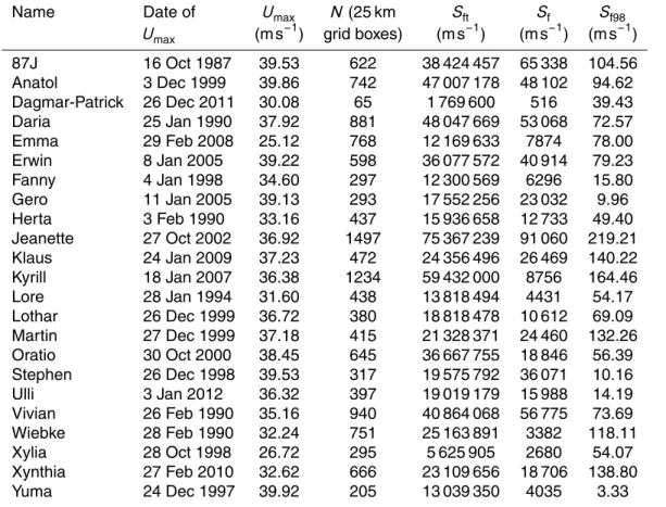
Table 1.The 23 severe storms highlighted by insurance experts in the period 1979–2012. The indicesU_max,N,S_ft,S_fandS_f98are defined in Sect. 3.1.

Name Date of U_max N(25 km S_ft S_f S_f98

U_max (m s−1) grid boxes) (m s−1) (m s−1) (m s−1)

87J 16 Oct 1987 39.53 622 38 424 457 65 338 104.56

Anatol 3 Dec 1999 39.86 742 47 007 178 48 102 94.62

Dagmar-Patrick 26 Dec 2011 30.08 65 1 769 600 516 39.43

Daria 25 Jan 1990 37.92 881 48 047 669 53 068 72.57

Emma 29 Feb 2008 25.12 768 12 169 633 7874 78.00

Erwin 8 Jan 2005 39.22 598 36 077 572 40 914 79.23

Fanny 4 Jan 1998 34.60 297 12 300 569 6296 15.80

Gero 11 Jan 2005 39.13 293 17 552 256 23 032 9.96

Herta 3 Feb 1990 33.16 437 15 936 658 12 733 49.40

Jeanette 27 Oct 2002 36.92 1497 75 367 239 91 060 219.21

Klaus 24 Jan 2009 37.23 472 24 356 496 26 469 140.22

Kyrill 18 Jan 2007 36.38 1234 59 432 000 8756 164.46

Lore 28 Jan 1994 31.60 438 13 818 494 4431 54.17

Lothar 26 Dec 1999 36.72 380 18 818 478 10 612 69.09

Martin 27 Dec 1999 37.18 415 21 328 371 24 460 132.26

Oratio 30 Oct 2000 38.45 645 36 667 755 18 846 56.39

Stephen 26 Dec 1998 39.53 317 19 575 792 36 071 10.16

Ulli 3 Jan 2012 36.32 397 19 019 179 15 988 14.19

Vivian 26 Feb 1990 35.16 940 40 864 068 56 775 73.69

Wiebke 28 Feb 1990 32.24 751 25 163 891 3382 118.11

Xylia 28 Oct 1998 26.72 295 5 625 905 2680 54.07

Xynthia 27 Feb 2010 32.62 666 23 109 656 18 706 138.80

Yuma 24 Dec 1997 39.92 205 13 039 350 4035 3.33

(26)

NHESSD

2, 2011–2048, 2014

Title Page

Tables Figures

◭ ◮

Back Close

Full Screen / Esc

Discussion

P

a

per

|

D

iscussion

P

a

per

|

Discussion

P

a

per

|

Discuss

ion

P

a

per

|

Table 2. The number of storms in categories A, B and C for each index, where category A storms are severe and not meteorologically extreme, category B storms are meteorologi-cally extreme and not severe, category C storms are severe and meteorologimeteorologi-cally extreme, and category D storms are not severe and not meteorologically extreme.

Index n_A n_B n_C

U_max 8 27 15

N 8 27 15

S_ft 6 27 17

S_f 13 27 10

Sf98 10 27 13

(27)

NHESSD

2, 2011–2048, 2014

Title Page

Tables Figures

◭ ◮

Back Close

Full Screen / Esc

Discussion

P

a

per

|

D

iscussion

P

a

per

|

Discussion

P

a

per

|

Discuss

ion

P

a

per

|

Table 3.Parameter estimates and standard errors for the mean function described in Sect. 5.

Parameter logσ β0 β1 β2 γelev,0 γlon,0 γlat,0 γlon:lat,0

Estimate −1.6023 −1.3411 1.8340 −0.1266 0.0056 0.1382 −0.8135 0.2734 Standard error 0.0007 0.0007 0.0007 0.0008 0.0007 0.0007 0.0007 0.0007

Parameter γelev,1 γlon,1 γlat,1 γlon:lat,1 γelev,2 γlon,2 γlat,2 γlon:lat,2

Estimate −0.0030 −0.1506 0.5199 −0.1883 0.0004 0.0292 −0.0832 0.0321 Standard error 0.0006 0.0007 0.0007 0.0007 0.0002 0.0008 0.0007 0.0007

(28)

NHESSD

2, 2011–2048, 2014

Title Page

Tables Figures

◭ ◮

Back Close

Full Screen / Esc

Discussion

P

a

per

|

D

iscussion

P

a

per

|

Discussion

P

a

per

|

Discuss

ion

P

a

per

|

(29)

NHESSD

2, 2011–2048, 2014

Title Page

Tables Figures

◭ ◮

Back Close

Full Screen / Esc

Discussion

P

a

per

|

D

iscussion

P

a

per

|

Discussion

P

a

per

|

Discuss

ion

P

a

per

|

Fig. 2.Footprints of storms 4769, 4773, 4782 and 4774 made by taking the maximum gusts over the whole domain (contaminated).

(30)

NHESSD

2, 2011–2048, 2014

Title Page

Tables Figures

◭ ◮

Back Close

Full Screen / Esc

Discussion

P

a

per

|

D

iscussion

P

a

per

|

Discussion

P

a

per

|

Discuss

ion

P

a

per

|

(31)

NHESSD

2, 2011–2048, 2014

Title Page

Tables Figures

◭ ◮

Back Close

Full Screen / Esc

Discussion

P

a

per

|

D

iscussion

P

a

per

|

Discussion

P

a

per

|

Discuss

ion

P

a

per

|

Fig. 4. (a)Conceptual diagram of meteorological extremity and severity. All 5730 storms can be classified into 1 of 4 categories: severe and not meteorologically extreme (category A), meteorologically extreme and not severe (category B), severe and meteorologically extreme (category C) and not severe and not meteorologically extreme (category D). The number of storms in category A, B and C must total 50 (n_A+n_B+n_C=50).(b)The number of storms in category C (n_C) for the topn_B+n_Cstorms, for indexS_ft.