Parametric representation of the cloud droplet spectra for LES warm bulk microphysical schemes

(1)

ACPD

9, 17633–17663, 2009

Parametric representation of the cloud droplet spectra

O. Geoffroy et al.

Title Page

Abstract Introduction

Conclusions References

Tables Figures

◭ ◮

Back Close

Full Screen / Esc

Printer-friendly Version

Interactive Discussion Atmos. Chem. Phys. Discuss., 9, 17633–17663, 2009

www.atmos-chem-phys-discuss.net/9/17633/2009/ © Author(s) 2009. This work is distributed under the Creative Commons Attribution 3.0 License.

Atmospheric Chemistry and Physics Discussions

This discussion paper is/has been under review for the journalAtmospheric Chemistry and Physics (ACP). Please refer to the corresponding final paper inACPif available.

Parametric representation of the cloud

droplet spectra for LES warm bulk

microphysical schemes

O. Geoffroy1, J.-L. Brenguier2, and F. Burnet2

1

Royal Netherlands Meteorological Institute (KNMI), De Bilt, The Netherlands 2

GAME/CNRM (M ´et ´eo-France, CNRS), Toulouse, France

Received: 16 July 2009 – Accepted: 6 August 2009 – Published: 25 August 2009

Correspondence to: O. Geo_ffroy (geo_ffroy@knmi.nl)

(2)

ACPD

9, 17633–17663, 2009

O. Geoffroy et al.

Title Page

Tables Figures

◭ ◮

Back Close

Full Screen / Esc

Interactive Discussion

Abstract

Parametric functions are currently used to represent droplet spectra in clouds and to develop bulk parameterizations of the microphysical processes and of their interactions with radiation. The most frequently used parametric functions are the Lognormal and the Generalized Gamma which have three and four independent parameters,

respec-5

tively. In a bulk parameterization, two parameters are constrained by the total droplet number concentration and the liquid water content. In the Generalized Gamma func-tion, one parameter is specified a priori, and the fourth one, like the third parameter of the Lognormal function, shall be tuned, for the parametric function to statistically best fit observed droplet spectra.

10

These parametric functions are evaluated here using droplet spectra collected in non-or slightly precipitating stratocumulus and shallow cumulus. Optimum values of the tuning parameters are derived by minimizing either the absolute or the relative error for successively the first, second, fifth, and sixth moments of the droplet size distribution. A trade-off value is also proposed that minimizes both absolute and relative errors

15

for the four moments concomitantly. Finally, a parameterization is proposed in which the tuning parameter depends on the liquid water content. This approach significantly improves the fit for the smallest and largest values of the moments.

1 Introduction

Cloud particles are represented by their size distribution also referred to as spectrum.

20

In the liquid phase, the spectrum originates from activation of cloud condensation nu-clei (CCN), mainly at cloud base. Hence it expends from submicron particles for the smallest activated CCNs to about 10µm in radius for the giant ones. As particles grow by condensation, the spectrum gets narrower because the growth rate of a droplet is inversely proportional to its size. Higher in a cloud, spectral narrowing is

coun-25

(3)

ACPD

9, 17633–17663, 2009

O. Geoffroy et al.

Title Page

Tables Figures

◭ ◮

Back Close

Full Screen / Esc

Interactive Discussion experience different growth histories along different trajectories, some ascending

adi-abatically from cloud base, while others undergo dilution with environmental air and partial evaporation. New CCNs can also be activated higher than cloud base, when moist and clear air is entrained in an updraft, hence initiating small droplets. When the biggest droplets reach a radius of about 20µm, collision and coalescence

gener-5

ate drizzle particles (from 20 to a few 100µm). If the cloud is sufficiently deep and the liquid water content large enough, droplets and drops continue to collide to form precipitation drops (mm). The maximum drop radius, of the order of 4 mm, is limited by break-up, either following a collision or spontaneously for the biggest drops. The total number concentration spans over a large range, because millions of droplets are

nec-10

essary to form a drop. It thus evolves from up to 1000 cm−3 for droplets in a polluted environment, to a few per cubic meter for precipitation drops. Because the number concentration of activated CCN, the convective cell trajectories, the series of mixing events and the resulting growth histories by condensation, collection and break-up are infinitely diverse, cloud particle spectra exhibit all kinds of shapes (Warner, 1969a, b,

15

1970, 1973a, b).

The cloud droplet size distribution (CDSD) is expressed as a concentration density,

n(r)dr, i.e. number density of droplets per volume (or per mass) of air, and per unit size. To summarize the properties of a size distribution, one commonly uses a moment of the distributionMp, or the mean radius of thepthmomentrp:

20

M_p= ∞ Z

0

rpn(r)dr, (1)

rp=

M_p

N

_p1

(2) whereN=M0is the total number concentration.

To interpret microphysical observations, examine the interactions between cloud mi-crophysics and other physical processes, and numerically simulate these interactions,

(4)

ACPD

9, 17633–17663, 2009

O. Geoffroy et al.

Title Page

Tables Figures

◭ ◮

Back Close

Full Screen / Esc

Interactive Discussion parametric functions are frequently used to reduce the variety of the droplet spectral

shapes. The objective in this paper is to evaluate parametric functions that best repli-cate observed spectra on a statistical basis. The focus is on non-or slightly precipitating stratocumulus and shallow cumulus clouds.

After a brief description (Sect. 2) of bulk microphysics schemes, three frequently

5

used parametric functions are described in Sect. 3. The methodology for tuning the functions and the data sets on which tuning relies are detailed in Sects. 4 and 5, respectively. Section 6 addresses the specific issue of scaling up small scale mea-surements for characterizing cloud system properties. The results are then reported in Sect. 7, for fixed and variables values of the tuning parameters successively, before

10

the conclusions.

2 Bulk parameterizations and parametric functions

In a numerical model, the natural variability of the droplet spectra can be explicitly sim-ulated with “bin” microphysical schemes where the number distribution is discretized, from 30 to 200 size classes (Kogan, 1991). The computational cost of such schemes

15

however, prevents their use in large domain, high spatial resolution, cloud resolving models. Instead, bulk parameterizations have been developed. Indeed, even though spectra are diverse, one usually observe a transition from droplets to drops, in the size range where condensational growth becomes inefficient, while collection starts to become significant, namely between 20 and 50µm in radius. This size range also

cor-20

responds to a rapid increase of the particle fall velocity with the particle radius (∝r2). In a liquid phase bulk scheme, hydrometeors are thus distributed in two categories, the droplets that do not or slowly sediment, and the drops that precipitate more rapidly. This necessarily introduces errors and biases. The art in the development of bulk parame-terizations is therefore to carefully select the minimum number of well suited prognostic

25

(5)

ACPD

9, 17633–17663, 2009

O. Geoffroy et al.

Title Page

Tables Figures

◭ ◮

Back Close

Full Screen / Esc

Interactive Discussion Bulk parameterizations can be classified according to the number of particle

cate-gories, the threshold radius value that separates the catecate-gories, and the number of independent variables used to describe each category. For the liquid phase, they are currently limited to two hydrometeor categories, droplets and drops, but the threshold radius depends on the application. For simulation of deep clouds, the threshold radius

5

is generally set to about 40–50µm (Berry and Reinhardt, 1974; Seifert and Beheng, 2001), while for shallow clouds a lower threshold of 20–25µm is preferred (Khairoutdi-nov and Kogan, 2000). Note that all independent variables of a parameterization are not necessarily prognostic variables in a numerical model. For instance in Seifert and Beheng (2006), using a Gamma distribution to represent the droplet mass spectrum,

10

the parameterνc is set to 1; in Ackerman et al. (2008) using a Lognormal distribution,

the parameterσ_g is set to 1.5, although a value of 1.2 is recognized to better fit the observations. Original bulk schemes were limited to one prognostic variable per cate-gory: the water content,qcfor the droplets andqrfor the drops (or mixing ratio=q/ρa,

whereρ_a is the air density) (Kessler, 1969; Tripoli and Cotton, 1980). More recent

15

schemes rely on 4 prognostic variables, adding to the water contents the total number concentration in each category, Nc and Nr (Ziegler, 1985; Cohard and Pinty, 2000;

Khairoutdinov and Kogan, 2000; Seifert and Beheng, 2001). Beyond the total water content and total number concentration of particles in each category, there were a few attempts to introduce more variety by also predicting additional variables such as the

20

reflectivity, as in Milbrandt and Yau (2005). Table 1 summarizes the characteristics of existing bulk parameterizations for the liquid phase, with a focus on the description of the droplet category.

The physical processes that act as sources and sinks for the particle categories shall then be parameterized. The CCN activation process is a source for the droplet

cate-25

(6)

ACPD

9, 17633–17663, 2009

O. Geoffroy et al.

Title Page

Tables Figures

◭ ◮

Back Close

Full Screen / Esc

Interactive Discussion droplets and the collection between drops to form bigger drops (self-collection) are

also considered (Ziegler, 1985; Cohard et Pinty, 2000; Seifert and Beheng, 2006). In-deed, these two last processes do not affect the mass of condensed water in each category, but the number concentration, hence the mean size of the particles and their mean fall velocity.

5

It is also useful to notice that two methodologies were adopted to develop bulk pa-rameterizations. In the empirical approach (Khairoutdinov and Kogan, 2000), numer-ical simulations of clouds are performed with a bin microphysics scheme. Each grid box, at each time step, is then used as one realisation of the microphysical processes, from which bulk variables (q_c,q_r,N_c,N_r) and their evolution rates by CCN activation,

10

auto-conversion, accretion, and precipitation can be calculated. Empirical laws are then derived by minimization over the whole set of realisations. In such a case, the accuracy of the parameterization is limited by the performance of the bin microphysics scheme and the variable space explored by the simulations. Others (Liu and Daum, 2004) follow a more analytical approach in which the particle size distribution in each

15

category is represented by a parametric function. The stochastic collection equation is then analytically resolved to derive a formulation of the auto-conversion and accretion rates. In this case the accuracy of the solution mainly depends on the realism of the chosen parametric function. Note however, that coefficients of some “analytical type” bulk parameterizations are tuned empirically (Seifert and Beheng, 2001, 2006).

20

Some physical processes in a cloud model require additional information about cloud microphysics, beyond the prognostic number concentration (N=M0) and water content

(_∝M3). For instance, CCN activation is often parameterized using a diagnostic of the

peak supersaturation, that depends on the first moment of the size distribution M1,

also referred to as the droplet integral radius (Twomey, 1959). Radiative transfer

calcu-25

lations in clouds depend on light extinction that is proportional to the second moment

M2 of the droplet spectrum (Hansen and Travis, 1974). The sedimentation flux

(7)

ACPD

9, 17633–17663, 2009

O. Geoffroy et al.

Title Page

Tables Figures

◭ ◮

Back Close

Full Screen / Esc

Interactive Discussion (Roger and Yau, 1989), the sedimentation flux of particle number is proportional to the

second moment,M2, and the sedimentation flux of water content is proportional to the

fifth moment, M5. The radar reflectivity in a liquid phase cloud is proportional to M6

(Atlas, 1954). The width of the size distributionw=1/M0

q

M0M2−M12, or its dispersion d=N_·w/M1, have been used to establish relationships between the mean volume and

5

effective radii of the droplet spectrum for radiative transfer calculations (Liu and Daum, 2000). It is therefore not su_fficient for a microphysics bulk parameterization to accu-rately predict the auto-conversion and accretion rates; it must also provide accurate diagnostics of various integral properties of the cloud droplet spectrum, at least forM1, M2,M5,M6.

10

In summary, bulk parameterizations that are developed following an analytical ap-proach rely on a priori specified parametric functions for the description of the droplet spectra. Moreover, all bulk parameterizations, including those empirically tuned, also require a priori specified parametric functions to establish formal relationships between the prognostic moments of the droplet size distribution (M0andM3) and those used in

15

the parameterization of each microphysical process.

3 Commonly used parametric functions

To represent droplet size distributions, the most frequently used parametric functions are the Lognormal (Clark, 1976; Feingold et Levin, 1986) and the Generalized Gamma (Liu and Hallett, 1998; Cohard et Pinty, 2000). These two functions are convenient

20

because any of their moments can be expressed as a function of the parameters of the distribution.The Lognormal function

n_c(r)=N_√ 1

2πrlnσ_g exp



− 1 2

ln(r/rg)

lnσ_g

!2

(8)

ACPD

9, 17633–17663, 2009

O. Geoffroy et al.

Title Page

Tables Figures

◭ ◮

Back Close

Full Screen / Esc

Interactive Discussion has 3 independent parameters, the total number concentrationN, the geometric

stan-dard deviationσ_g, and the mean geometric radius r_g, where r_g=e<ln(r)>. Thepth mo-ment of the spectrum is directly related toN,σg, andrg via:

Mp=Nr p g exp

p2

2 (lnσg)

2

!

, (4)

and it is expressed as a function ofN,M3andσgas

5

M_p=N1−p/3M₃p/3exp p

2

−9 2 ln(σg)

2

!

. (5)

The Generalised Gamma function

n(r)=N α

Γ(ν)λ

αν_rαν₋1_exp(

−(λr)α) (6)

has 4 independent parameters, N, the slope parameter λand the two shape param-eters α and ν. The pth moment of the spectrum is directly related to N, λ, α and ν

10

via:

Mp= N λp

Γ(ν+pα)

Γ(ν) !

(7)

and it is expressed as a function ofN,M3,αandνas:

M_p=N1−p/3M₃p/3 Γ(ν+ p α)

Γ(ν+α3)

p 3

Γ(ν)p−33. (8)

The Generalized Gamma function includes the Gamma (or Golovin), the Exponential

15

(9)

ACPD

9, 17633–17663, 2009

O. Geoffroy et al.

Title Page

Tables Figures

◭ ◮

Back Close

Full Screen / Esc

Interactive Discussion Gamma function to represent the cloud droplet mass distribution (Berry and Reinhardt,

1974; Williams and Wojtowicz, 1982; Seifert and Beheng, 2001), which is equivalent of using a Generalized Gamma function with α=3 (hereafter referred to as GG3) for describing the particle number concentration distribution. In this paper, both values,

α=1 andα=3, are evaluated.

5

In summary, in the framework of a bulk parameterization with two prognostic vari-ables for the droplet category (M₀ and M₃), there is still one parameter to adjust, hereafter referred to as the tuning parameter, eitherσg for the Lognormal orνfor the

Generalised Gamma function, whereα has been specified to either 1 or 3.

4 Methodology

10

The objective in this paper is to determine which value of the tuning parameter al-low the parametric function to statistically best fit the observed droplet spectra. More specifically we will address the following questions.

– When a Lognormal, a GG1 or a GG3 function is used, and the tuning parameter is constant, what is the best value to use for this parameter?

15

– Is the accuracy improved if the tuning parameter is allowed to vary?

– In such a case how can it be diagnosed from the two prognostic variablesN and

q_c?

To answer these questions, a large sample of droplet spectra measured in diverse types of non- or slightly precipitating shallow clouds is used. The best fit to each

ob-20

served spectrum is obtained with either a Lognormal or a Generalized Gamma function that has the same droplet number concentration and liquid water content, and a value of the tuning parameter, σ_g for the Lognormal, ν1 for GG1 and ν3 for GG3, that

min-imizes the difference between an integral property of the observed spectrum and the one of the parametric function. The integral properties considered here areM1,M2,

(10)

ACPD

9, 17633–17663, 2009

O. Geoffroy et al.

Title Page

Tables Figures

◭ ◮

Back Close

Full Screen / Esc

M5,M6. For each one separately, the value of the tuning parameter that minimizes the

mean absolute error between the property value of the observed spectrum (xm) and

the one derived from the fitted parametric function (x_p) is calculated. The same pro-cedure is applied to the relative error, where the absoluteεabs and relative εrel errors

are defined as: εabs=xp−xm and εrel=xp/xm. The statistical adequacy of the tuning

5

parameter value is then evaluated for each moment successively. Since there is no reason for a single value of the tuning parameter to minimize the errors for the 4 mo-ments concomitantly, a trade-of value is also evaluated in terms of absolute and relative errors.

In the second step, a parameterization is proposed to allow the value of the tuning

10

parameter to vary, and the resulting errors, both absolute and relative, are calculated for comparison with the ones obtained in step 1.

5 The data sets

Cloud particle size distributions used in this study were collected during two airborne field experiments: The ACE-2 campaign took place in June and July 1997 to document

15

marine boundary layer stratocumulus clouds, north of the Canary islands (Brenguier et al., 2000). The RICO campaign took place in December 2004 and January 2005 to study shallow precipitating cumulus clouds of the coast of the Caribbean Island of Antigua and Barbuda within the Northeast Trades of the western Atlantic (Rauber et al., 2007).

20

The droplet spectra were measured with the Fast-FSSP, a droplet spectrometer that covers a range from 1 to about 20–25µm in radius (Brenguier et al., 1998). The droplet spectra are extended beyond 25µm with data from a PMS-OAP-200-X (PMS Inc, Boul-der Colorado, USA) during ACE-2 and a PMS-OAP-260-X during RICO. The 200-X measures drizzle particle sizes over 15 radius bins from 7.5 to 155µm, with a bin width

25

(11)

ACPD

9, 17633–17663, 2009

O. Geoffroy et al.

Title Page

Tables Figures

◭ ◮

Back Close

Full Screen / Esc

Interactive Discussion This value is selected because it corresponds to a bin limit in both the OAP-200-X and

-260-X and it is intermediate between the values used in most bulk parameterizations. A sensitivity study suggests that the selected threshold radius value has no noticeable impact on the results within the range from 27.5 to 37.5µm.

These two campaigns were selected because significant differences were expected

5

between the stratocumulus and the shallow cumulus regimes. The depth of the stra-tocumulus clouds in ACE-2 was a few hundreds of meters, while it reaches a few kilometres for the RICO shallow cumuli. In ACE-2, the droplet number concentration varied from less than 50 to more than 400 cm−3, while it was lower during RICO with values less than 100 cm−3 in most cases. Light precipitation was observed in ACE-2,

10

while it was slightly stronger in the RICO clouds. In general, the LWC in stratocumu-lus remains close to adiabatic up to cloud top (Brenguier et al., 2003; Pawlowska and Brenguier, 2003), while it is significantly diluted in the RICO cumulus clouds. Cloud sampled during RICO show indeed that peak LWC values decrease continuously with height down to about 50% of the adiabatic value 1 km above cloud base, while median

15

LWC values drop down to about 30% of the adiabatic within the first 200 m.

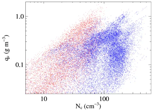
Droplet spectra were sampled at 1 Hz (a flight distance of about 100 m). Cloudy samples are defined as samples with a LWC greater than 0.025 g m−3 and a cloud droplet number concentration N_c greater than 5 cm−3. Figure 1 shows a scatter-plot of the droplet number concentration (M0) and the LWC (_∝M3), with di_fferent colours

20

for the ACE2 (blue) and the RICO (red) data sets. The number concentrations are lower in RICO, but the LWC values are similar in both data sets, up to 2 g m−3. Overall, the two campaigns provide a set of 27 623 cloud droplet spectra in total: 19 151 from 8 ACE-2 cases (fr9720, fr9721, fr9728, fr9730, fr9731, fr9733, fr9734, fr9735) and 8472 from 7 RICO cases (RF06, RF07, RF08, RF09, RF11, RF12, RF13), sampled at

25

(12)

ACPD

9, 17633–17663, 2009

O. Geoffroy et al.

Title Page

Tables Figures

◭ ◮

Back Close

Full Screen / Esc

6 From the small scale to the cloud system scale

In this exercise, the spatial scale is an important issue. Indeed, airborne cloud parti-cle spectrometers have a limited sampling section, so that a very tiny fraction of air is sampled along the flight track. For instance, the Fast-FSSP has a sampling section of 0.1 mm2. Droplet counts are therefore cumulated over 100 m for the measured

dis-5

tribution to become statistically significant (about 1000 droplets sampled at a number concentration of 100 cm−3). For drizzle and precipitation drops, the number concen-tration decreases exponentially with size, but the sampling section of the drizzle and precipitation particle spectrometers does not increase accordingly. One is thus tempted to increase the sample length, hence increase the number of sampled particles, to

bet-10

ter characterize a spectrum. Droplet spectra, however, are highly variable at scales smaller than 100 m (Pawlowska et al., 1997). This spatial variability raises two impor-tant issues when averaging spectra over long distances for characterizing cloud system representative properties.

First, the spatial variability is linearly smoothed out when cumulating particle counts

15

over a long sample and this may become an issue if the physical process of interest is highly non-linear. Although they are second order, the biases arising from using non-linear combinations of linearly averaged microphysical parameters may thus oc-casionally lead to flawed conclusions. A typical example is when characterizing the spectral width for studies of the collection process. Indeed, the droplet collection

(col-20

lision and coalescence) is highly sensitive to the presence of both small and large droplets in the same micro-volume of cloudy air. Thus it depends non-linearly on the width of the droplet spectrum. In cumulus clouds for instance, narrow droplet spec-tra are observed at all levels, but their mode increases from cloud base to the top. If droplet measurements are cumulated over flight legs ascending from the cloud base

25

(13)

ACPD

9, 17633–17663, 2009

O. Geoffroy et al.

Title Page

Tables Figures

◭ ◮

Back Close

Full Screen / Esc

Interactive Discussion on flight legs that are statistically homogeneous in term of spectral properties.

The second issue arises when averaging CDSD intensive properties, such as the radius of the pth moment instead of extensive1 properties such as the moment it-self. For instance the light extinction in a cloud depends on the second moment, as

σext=πQext M2=πQext Nr 2

2, where r2, is the mean radius of the 2nd moment or mean

5

surface radius of the droplet spectrum. The mean extinction in a cloud layer, is there-fore equal to_hσexti=πQexthM2i, which is different fromπQexthNi hr2i

2

. The latter formu-lation, however, is the most frequently used because observational data sets are often processed to derive the mean droplet number concentration and the mean surface ra-dius, or effective radius, instead of the mean second moment of the size distributions.

10

Diluted cloud volumes often show intensive properties that are quite di_fferent from the ones observed in undiluted volumes because of the impact of entrainment and mixing processes (Burnet and Brenguier, 2007). However, when using the second formula-tion, diluted volumes are given the same weight as the undiluted ones, while they very little contribute to the mean value of the corresponding moment.

15

In general, one shall therefore avoid averaging spectral properties such as any mean radius of the distribution or ratio of such variables as the k coefficient in Martin et al. (1994) that do not depend on the droplet concentration, hence might overemphasize the contributions of highly diluted cloud volumes. The tuning of the parametric functions described hereafter is thus based on moments of the size distribution instead of mean

20

radii of the moments, and 4 moments (M1,M2,M5andM6) are considered separately.

1

(14)

ACPD

9, 17633–17663, 2009

O. Geoffroy et al.

Title Page

Tables Figures

◭ ◮

Back Close

Full Screen / Esc

7 Tuning of the parametric functions

7.1 Constant tuning parameter

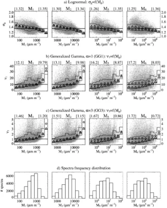
Figure 2 summarizes the analysis. The first three rows show scatter-plots of the tuning parameter values for the four moments, from left to right. The range of variation of the moment values has been divided in 10 classes on a Log scale. The first row is for the

5

Lognormal parametric function, the second one for the Generalized Gamma withα=1 (GG1), and the third one for the Generalized Gamma with α=3 (GG3). The last row shows the number of samples in each moment class.

Each grey point represents the value of the tuning parameter that best fits the speci-fied moment of an observed spectrum. Superimposed to the scatter-plot, two thin lines

10

represent the 25th and 75th percentiles of the tuning parameter values in each moment class. The circles and triangles are the tuning parameter values that minimize, in each moment class, the arithmetic and the geometric standard deviation of the absolute and relative errors, respectively. On top of each graph, the number in brackets on the left (right) hand side is the tuning parameter value that minimizes the absolute (relative)

15

error over the whole range of variation of the specified moment.

For the Lognormal distribution, the top row suggests that aσ_gvalue between 1.3 and 1.4 provides accurate estimations, for the moment values that are the most frequently observed, i.e. 103µm cm−3forM1, 5.10

3

µm2cm−3forM2, from 10 6

to 2.107µm5cm−3 forM5 and from 10

7

to 2.108µm6cm−3 for M6. For M1 and M2, however, this value

20

underestimates the optimumσ_g value at small moment values, hence overestimates the small moment values, and inversely for the large moment values. For the higher moments,M5andM6, the optimumσg value does not vary significantly with the value

of the moment. The sensitivity test to the radius threshold value that separates droplets from drops in the bulk scheme reveals that these two higher moments are more

sensi-25

(15)

parameteri-ACPD

9, 17633–17663, 2009

O. Geoffroy et al.

Title Page

Tables Figures

◭ ◮

Back Close

Full Screen / Esc

Interactive Discussion zation of cloud droplet sedimentation (Ackerman et al., 2008).

For the Generalised Gamma distribution, the results are similar, with optimum values of the tuning parameterνof the order of 10 for GG1 and slightly larger than 1 for GG3, although the trends are reversed compared to the Lognormal since increasing values of theνparameters correspond to narrower spectra. A value ofν3equal to 1 corresponds

5

in the formulation of the auto-conversion in Seifert and Beheng (2006, Eq. 4) to aν_c

value equal to 0, which is commonly used.

This set of scatter-plots suggests that there is no single parameter value that min-imizes both errors for the 4 moments concomitantly. The optimum value indeed de-pends on the application and one might select aM1 optimum value for the prognostic

10

of peak supersaturation in a CCN activation scheme, a M2 specific one for radiative

transfer and the sedimentation flux of particle number concentration, aM5specific one

for the sedimentation flux of particle water content, and aM6 specific one for the

re-trieval of cloud properties from a radar reflectivity.

It might be questionable, and less practicable, to use different values of the tuning

pa-15

rameter for the analytical function that describes the droplet distribution in a numerical model, although this is a common practice when using in a numerical model parame-terizations of diverse origins, hence relying on different values of the tuning parameter or even different parametric functions. For instance the bulk microphysical schemes tested by the GCSS boundary layer working group are based on a Lognormal function

20

for parameterization of droplet sedimentation (Ackerman et al., 2008), whereas the au-toconversion scheme often relies on different hypotheses. Some authors use different distribution hypotheses in the same process parameterization (see Table 1 in Gilmore and Straka, 2008). For better consistency, we propose a compromise that partly sat-isfies all types of applications. A trade-off value of the tuning parameter is derived

25

as:

p∗= 1 8n

X

i ,j,kni ,jpi ,j,k, (9)

(16)

ACPD

9, 17633–17663, 2009

O. Geoffroy et al.

Title Page

Tables Figures

◭ ◮

Back Close

Full Screen / Esc

j_∈[1,2,5,6] stands for the moment, andk_∈[1,2], corresponds to either the absolute or relative error. ni ,j, is the number of samples in classi of the momentMj andpi ,j,k, is

the optimum tuning parameter value in the classi of the moment j, for the absolute and relative errors, respectively.

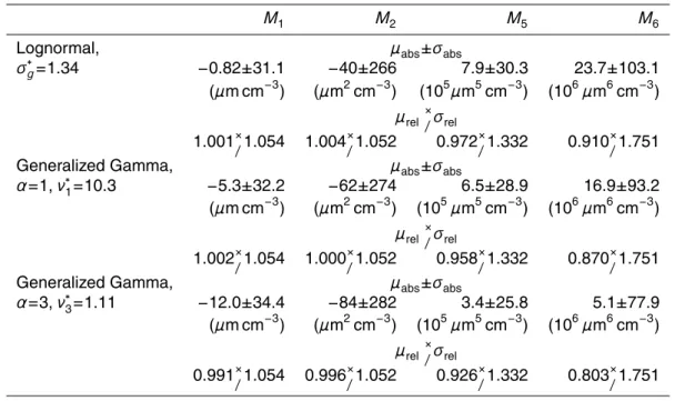
This trade-o_ffvalue of the tuning parameter,σ∗g=1.34 for the Lognormal,ν∗1=10.3 for

5

GG1 andν∗₃=1.11 for GG3, is represented in Fig. 2 by a horizontal bar and it is reported in Table 2, with the resulting offset and standard deviations of the absolute and relative errors.

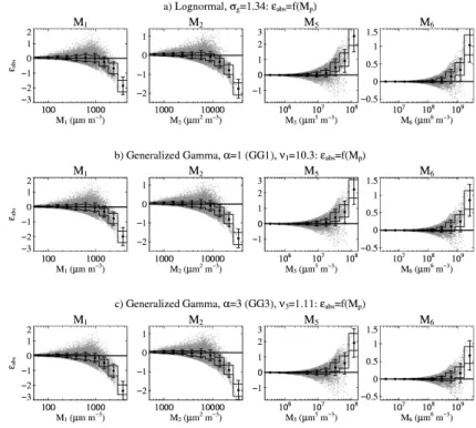
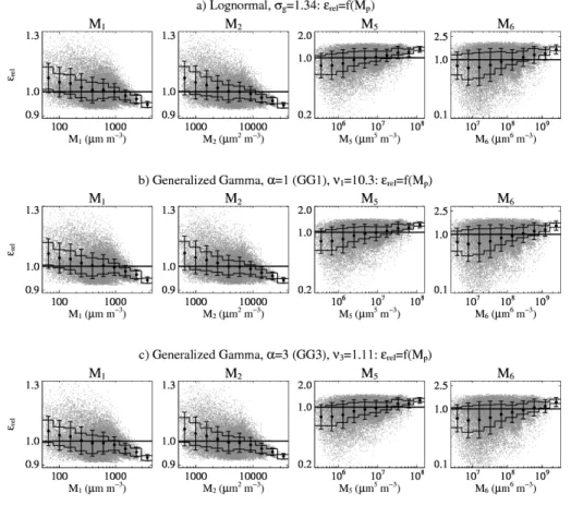
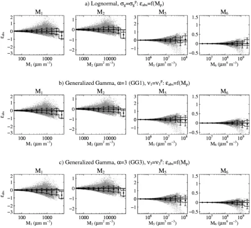
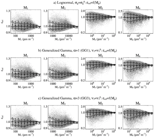
Figure 3 shows scatter-plots of the absolute errors in each moment class, as in Fig. 2, for the Lognormal (first row), the GG1 (second row) and the GG3 (third row) parametric

10

functions. The grey points represent the error for each sampled spectrum, the thin lines denote the 25th and the 75th percentiles of the absolute error distribution in each class, and the circle and error bars indicate the arithmetic mean (offset) and standard deviation of the absolute error values in each class. Note that for practical reasons, the error values are normalized in each graph, as specified in the figure caption. Figure 4

15

is similar for the relative errors, although errors are not normalized in this case. These figures confirm that a single parameter value provides accurate descriptions of the droplet spectra in the most common range of moment values, but significantly deviates at low moment values for the relative error and high moment values for both errors, although such samples are less frequently observed.

20

7.2 Variable tuning parameter

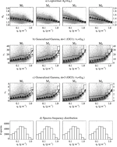
In a second step, we explore the potential of diagnosing the tuning parameter, using the prognostic variables of a bulk parameterization, i.e.N orq_c. The tuning parameter shows the greatest sensitivity to the LWC. This is illustrated in Fig. 5 that is similar to Fig. 2, except that the x-axis now represents the LWC.

25

(17)

ACPD

9, 17633–17663, 2009

O. Geoffroy et al.

Title Page

Tables Figures

◭ ◮

Back Close

Full Screen / Esc

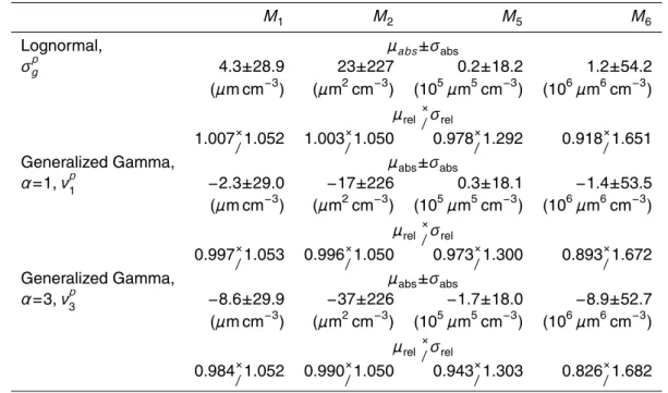
Interactive Discussion and the GG3 successively, leading to the following parameterizations:

σ_gp=−0.056_·ln(qc)+1.24, (10)

νp₁ =14.5_·qc+6.7, (11)

νp₃ =1.58·qc+0.72, (12)

whereqc is expressed in g m−3. They are represented in each graph of Fig. 5 by a

5

thick line.

Figures 6 and 7, similar to Figs. 3 and 4 show the improvement on the absolute and relative errors, respectively, in each moment class. The o_ffsets and standard devia-tions of the absolute and relative errors over the whole range of moment values are summarized in Table 3.

10

The comparison with Table 2, attests that both the absolute and relative errors have been reduced in term of offset and standard deviation, although the main improvement is for the absolute error at large values of the moments (Figs. 3 and 6), and for the relative error at both small and large values of the moments (Figs. 4 and 7).

8 Summary and conclusions

15

Droplet spectra measured in stratocumulus and shallow cumulus clouds have been examined to fit three parametric functions, i.e. the Lognormal, and the Generalized Gamma functions with α=1 and α=3, successively, that are frequently used in bulk parameterizations of the microphysics to represent droplet size distributions.

These functions have three independent parameters. Two are constrained by the

val-20

ues of the droplet number concentration and liquid water content. An optimum value of the third parameter, σ_g for the Lognormal, ν1 for the GG1 and ν3 for the GG3, has

(18)

ACPD

9, 17633–17663, 2009

O. Geoffroy et al.

Title Page

Tables Figures

◭ ◮

Back Close

Full Screen / Esc

Interactive Discussion using integral properties of the droplet spectra, namely 4 moments of the size

distribu-tion,M1 that is used in CCN activation schemes, M2 in radiative transfer calculations

and droplet sedimentation parameterization,M5 for parameterization of droplet

sedi-mentation, andM6for radar reflectivity calculations.

The range of variation of each moment has been divided in 10 classes on a Logscale

5

and the arithmetic and geometric means of the optimum parameter values have been calculated in each class. The absolute and relative errors have similarly been quanti-fied in each class, and over the whole range of variation of each moment. As expected, the optimum parameter values however are slightly different depending on which inte-gral property is used for the minimization. A trade-offparameter value has then been

10

proposed, that minimizes both the absolute and the relative errors on the 4 moments of the distributions.

In a second step, parameterizations are proposed where the optimum parameter value depends on the LWC, and the absolute and relative errors have been quantified for each moment separately. Such a varying tuning parameter slightly improves both

15

the absolute and relative errors for the moment values that are the most frequently observed, and it significantly improves the error at the lowest and largest values of the moments.

The potential of using the third parameter as a prognostic variable in a bulk scheme has been explored, but because of the large variability of spectral shapes and the

20

diversity of physical processes that are responsible for this variability, condensational growth, mixing and evaporation, droplet scavenging, and collection, we have not been able to isolate one process that could be considered as the most determinant. Further analysis or numerical simulations with bin microphysical schemes might help at solving the issue. However, considering the limitations inherent to the bulk approach, one might

25

also conclude that the accuracy of the parameterizations proposed here is sufficient for most of the topics that can be addressed with a bulk scheme.

(19)

Frame-ACPD

9, 17633–17663, 2009

O. Geoffroy et al.

Title Page

Tables Figures

◭ ◮

Back Close

Full Screen / Esc

Interactive Discussion work program project EUCAARI (European Integrated project on Aerosol Cloud Climate and

Air Quality interactions) No 036833-2. We thank Pier Siebesma for his comments which helped to improve the manuscript.

References

Ackerman, A. S., van Zanten, M. C., Stevens, B., Savic-Jovcic, V., Bretherton, C. S., Chlond, A.,

5

Gloaz, J.-G., Jiang, H., Khairoutdinov, M., Krueger, S. K., Lewellen, D. C., Lock, A., Moeng, C.-H., Nakamura, K., Petters, M. D., Snider, J. R., Weinbrecht, S., and Zulauf, M.: Large-eddy simulations of a drizzling, stratocumulus-topped marine boundary layer, Mon. Weather Rev., 137, 1083–1110, 2008.

Atlas, D.: The estimation of cloud parameters by radar, J. Meteorol., 11, 309–317, 1954.

10

Berry, E. X. and Reinhardt, R. L.: An analysis of cloud drop growth by collection Part II. Single initial distributions, J. Atmos. Sci., 31, 1825–1831, 1974.

Brenguier, J.-L., Bourrianne, T., de Araujo Coelho, A., Isbert, R. J., Peytavi, R., Trevarin, D., and Weschler, P.: Improvements of droplet distribution size measurements with the fast-FSSP (forward scattering spectrometer probe), J. Atmos. Ocean. Tech., 15, 1077–1090, 1998.

15

Brenguier, J.-L., Pawlowska, H., Sch ¨uller, L., Preusker, R., Fischer, J., and Fouquart, Y.: Ra-diative properties of boundary layer clouds: droplet effective radius versus number concen-tration, J. Atmos. Sci., 57, 803–821, 2000.

Brenguier, J.-L., Pawlowska, H., and Sch ¨uller, L. J.: Cloud microphysical and radiative proper-ties for parameterization and satellite monitoring of the indirect e_ffect of aerosol on climate,

20

J. Geophys. Res., 108, 8632, doi:10.1029/2002JD002682, 2003.

Burnet, F. and Brenguier, J.-L.: Observational study of the entrainment-mixing process in warm convective clouds, J. Atmos. Sci., 64, 1995–2011, 2007.

Clark, T. L.: Use of log-normal distributions for numerical calculation of condensation and col-lection, J. Atmos. Sci., 33, 810–821, 1976.

25

Cohard, J.-M. and Pinty, J.-P.: A comprehensive warm microphysical bulk scheme, part I: De-scription and selective tests, Q. J. Roy. Meteor. Soc., 126, 1815–1842, 2000.

(20)

ACPD

9, 17633–17663, 2009

O. Geoffroy et al.

Title Page

Tables Figures

◭ ◮

Back Close

Full Screen / Esc

Interactive Discussion Gilmore, M. S. and Straka, J. M.: The Berry and Reinhardt autoconversion : A digest. J. Appl.

Meteorol., 47, 375–396, 2008.

Hansen, J. E. and Travis, L. D.: Light scattering in planetary atmospheres, Space Sci. Rev., 16, 527–610, 1974.

Kessler, E.: On the Distribution and Continuity of Water Substance in Atmospheric Circulations,

5

Meteor. Monogr., 32, Amer. Meteor. Soc., 84 pp., 1969.

Khairoutdinov, M. and Kogan, Y.: A new cloud physics parameterization in a large-eddy simu-lation model of marine stratocumulus, Mon. Weather Rev., 128, 229–243, 2000.

Kogan, Y.: The simulation of a convective cloud in a 3-D model with explicit microphysics. Part I: Model description and sensitivity experiments, J. Atmos. Sci., 48, 1160–1189, 1991.

10

Martin, G. M., Johnson, D. W., and Spice, A.: The measurement and parameterization of effective radius of droplets in warm stratocumulus clouds, J. Atmos. Sci., 51, 1823–1842, 1994.

Liu, Y. and Hallett, J.: On size distributions of cloud droplets growing by condensation: A new conceptual model, J. Atmos. Sci., 55, 527–536, 1998.

15

Liu, Y. and Daum, P. H.: Spectral dispersion of cloud droplet size distributions and the parame-terization of cloud droplet effective radius, Geophys. Res. Lett., 27, 1903–1906, 2000. Liu, Y. and Daum, P. H.: Parameterization of the autoconversion process. Part I: Analytical

formulation of the Kessler-type parameterizations, J. Atmos. Sci., 61, 1539–1548, 2004. Manton, M. J. and Cotton, W. R.: Formulation of approximate equations for modeling moist

20

deep convection on the mesoscale, Atmos. Sci., 266, Dept. of Atmos. Sci., Colorado State University, 1977.

Milbrandt, J. A. and Yau, M. K.: A multimoment bulk microphysics parameterization. Part II: A proposed three-moment closure and scheme description, J. Atmos. Sci., 62, 3065–3081, 2005.

25

Pawlowska, H., Brenguier, J.-L., and Salut, G.: Optimal non-linear estimation for cloud particle measurements, J. Atmos. Ocean. Tech., 14, 88–104, 1997.

Pawlowska, H. and Brenguier, J.-L.: An observational study of drizzle formation in stratocu-mulus clouds for general circulation model (GCM) parameterizations, J. Geophys. Res., 108(D15), 8630, doi:10.1029/2002JD002679, 2003.

30

Rogers, R. R. and Yau, M. K.: A Short Course in Cloud Physics, Third edition, International Series in Natural Philosophy, Pergammon Press, 293 pp., 1989.

(21)

ACPD

9, 17633–17663, 2009

O. Geoffroy et al.

Title Page

Tables Figures

◭ ◮

Back Close

Full Screen / Esc

Interactive Discussion Jensen, J. B., Lasher-Trapp, S. G., Mayol-Bracero, O. L., Vali, G., Anderson, J. R., Baker,

B. A., Bandy, A. R., Burnet, F., Brenguier, J.-L., Brewer, W. A., Brown, P. R. A., Chuang, P., Cotton, W. R., Di Girolamo, L., Geerts, B., Gerber, H., G ¨oke, S., Gomes, L., Heikes, B. G., Hudson, J. G., Kollias, P., Lawson, R. P., Krueger, S. K., Lenschow, D. H., Nuijens, L., O’Sullivan, D. W., Rilling, R. A., Rogers, D. C., Siebesma, A. P., Snodgrass, E., Stith, J. L.,

5

Thornton, D. C., Tucker, S., Twohy, C. H., and Zuidema, P.: Rain in shallow cumulus over the ocean: The RICO campaign, B. Am. Meteorol. Soc., 88, 1912–1928, 2007.

Seifert, A. and Beheng, K. D.: A double-moment parameterization for simulating autoconver-sion, accretion and self-collection, Atmos. Res, 59–60, 265–281, 2001.

Seifert, A. and Beheng, K. D.: A two-moment cloud microphysics parameterization for

mixed-10

phase clouds. Part 1: Model description, Meteorol. Atmos. Phys., 92, 45–66, 2006.

Tripoli, G. J. and Cotton, W. R.: A numerical investigation of several factors contributing to the observed variable intensity of deep convection over South Florida, J. Atmos. Sci., 19, 1037–1063, 1980.

Twomey, S.: The nuclei of natural cloud formation. Part II: The supersaturation in natural clouds

15

and the variation of cloud droplet concentration, Geofys. Pura. Appl., 43, 243–249, 1959. Warner, J.: The microstructure of cumulus clouds. Part I. General features of the droplet

spec-trum, J. Atmos. Sci., 26, 1049–1059, 1969a.

Warner, J.: The microstructure of cumulus clouds. Part II. The effect on droplet size distribution of cloud nucleus spectrum and updraft velocity, J. Atmos. Sci., 26, 1272–1282, 1969b.

20

Warner, J.: The microstructure of cumulus clouds. Part III. The nature of the updraft, J. Atmos. Sci., 27, 682–688, 1970.

Warner, J.: The microstructure of cumulus clouds. Part IV. The effect on the droplet spectrum of mixing between cloud and environment, J. Atmos. Sci., 30, 256–261, 1973a.

Warner, J.: The microstructure of cumulus clouds. Part V. Changes in droplet size distribution

25

with cloud age, J. Atmos. Sci., 30, 1724–1726, 1973b.

Williams, R. and Wojtowicz, P. J.: A Simple Model for Droplet Size Distribution in Atmospheric Clouds, J. Appl. Meteorol., 21, 1042–1044, 1982.

Ziegler, C. L.: Retrieval of thermal and microphysical variables in observed convective storms. Part I: Model development and preliminary testing, J. Atmos. Sci., 42, 1487–1509, 1985.

(22)

ACPD

9, 17633–17663, 2009

O. Geoffroy et al.

Title Page

Tables Figures

◭ ◮

Back Close

Full Screen / Esc

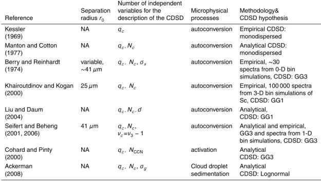
Interactive Discussion Table 1.Typical bulk parameterizations using two particle categories with, from left to right, the

value of the threshold radius between the two categories, the number of independent variables for the description of the droplet size distribution (CDSD), the parameterized microphysical pro-cesses, the methodology adopted for the development of the parametrization, and the CDSD parametric representation.

Number of independent

Separation variables for the Microphysical Methodology& Reference radiusr0 description of the CDSD processes CDSD hypothesis

Kessler NA qc autoconversion Empirical CDSD:

(1969) monodispersed

Manton and Cotton NA qc, Nc autoconversion Analytical CDSD:

(1977) monodispersed

Berry and Reinhardt variable, qc, Nc,σx autoconversion Empirical,∼30

(1974) _∼41µm spectra from 0-D bin

simulations, CDSD: GG3 Khairoutdinov and Kogan 25µm qc, Nc autoconversion Empirical, 100 000 spectra

(2000) from 3-D bin simulations of

Sc, CDSD: GG1 Liu and Daum NA qc, Nc, d autoconversion Analytical,

(2004) CDSD: GG1

Seifert and Beheng 41µm qc, Nc, autoconversion Analytical and empirical,

(2001, 2006) νc=ν3−1 GG3 and spectra from 1-D

bin simulations, CDSD: GG3 Cohard and Pinty NA qc, NCCN activation Analytical

(2000) CDSD: GG3

Ackerman NA qc, Nc,σg Cloud droplet Analytical

(23)

ACPD

9, 17633–17663, 2009

O. Geoffroy et al.

Title Page

Tables Figures

◭ ◮

Back Close

Full Screen / Esc

Interactive Discussion Table 2. Values of the arithmetic meanµ_absand the arithmetic standard deviationσ_absof the

absolute errors and of the geometric meanµ_rel and the geometric standard deviation σ_rel of the relative errors calculated for M₁, M₂, M₅, M₆, for the Lognormal, the GG1 and the GG3 parametric functions, when using the constant trade-off tuning parameters values,σ∗_g for the Lognormal,ν∗₁for the GG1 andν∗₃for the GG3.

M₁ M₂ M₅ M₆

Lognormal, µ_abs±σ_abs

σ∗_g=1.34 −0.82±31.1 −40±266 7.9±30.3 23.7±103.1 (µm cm−3) (µm2cm−3) (105µm5cm−3) (106µm6cm−3)

µrel×_/σrel

1.001×_/1.054 1.004×_/1.052 0.972×_/1.332 0.910×_/1.751 Generalized Gamma, µabs±σabs

α=1,ν∗₁=10.3 ₋5.3_±32.2 ₋62_±274 6.5_±28.9 16.9_±93.2

(µm cm−3) (µm2cm−3) (105µm5cm−3) (106µm6cm−3)

µrel×_/σrel

1.002×_/1.054 1.000×_/1.052 0.958×_/1.332 0.870×_/1.751 Generalized Gamma, µ_abs±σ_abs

α=3,ν∗₃=1.11 ₋12.0_±34.4 ₋84_±282 3.4_±25.8 5.1_±77.9

µ_rel×_/σ_rel

0.991×

/1.054 0.996

×

/1.052 0.926

×

/1.332 0.803

×

(24)

ACPD

9, 17633–17663, 2009

O. Geoffroy et al.

Title Page

Tables Figures

◭ ◮

Back Close

Full Screen / Esc

Interactive Discussion Table 3.Same as Table 2 when using the variable tuning parameter parameterizations,σp_gfor

the Lognormal,νp₁for the GG1 andνp₃for the GG3.

M1 M2 M5 M6

Lognormal, µ_abs±σ_abs

σp_g 4.3±28.9 23±227 0.2±18.2 1.2±54.2

µrel×_/σrel

1.007×_/1.052 1.003×_/1.050 0.978×_/1.292 0.918×_/1.651 Generalized Gamma, µ_abs±σ_abs

α=1,νp₁ −2.3±29.0 −17±226 0.3±18.1 −1.4±53.5

µ_rel×

/σrel 0.997×

/1.053 0.996

×

/1.050 0.973

×

/1.300 0.893

×

/1.672 Generalized Gamma, µ_abs_±σ_abs

α=3,νp₃ ₋8.6_±29.9 ₋37_±226 ₋1.7_±18.0 ₋8.9_±52.7

µ_rel×_/σ_rel

0.984×

/1.052 0.990

×

/1.050 0.943

×

/1.303 0.826

×

(25)

ACPD

9, 17633–17663, 2009

O. Geoffroy et al.

Title Page

Tables Figures

◭ ◮

Back Close

Full Screen / Esc

Interactive Discussion Fig. 1. Scatter-plot of the droplet number concentration, N_c, and the LWC, q_c, for droplet

(26)

ACPD

9, 17633–17663, 2009

O. Geoffroy et al.

Title Page

Tables Figures

◭ ◮

Back Close

Full Screen / Esc

Interactive Discussion Fig. 2. Scatter-plots (grey points) of the tuning parameter values as a function, from left to right, of theM₁,M₂,M₅,

(27)

ACPD

9, 17633–17663, 2009

O. Geoffroy et al.

Title Page

Tables Figures

◭ ◮

Back Close

Full Screen / Esc

Interactive Discussion Fig. 3. Scatter-plots (grey points) of the absolute errors between the observed spectrum

mo-ment value and the one of the parametric function using the trade-offvalue of the tuning param-eterσ∗_g=1.34 for the Lognormal function (top row),ν∗₁=10.3 for GG1 (2nd row), andν∗₃=1.11 for GG3 (3rd row), as a function of the moment values. The X-axis is divided in 10 classes as in Fig. 2. The thin lines denote the 25th and the 75th percentiles of the absolute error distribution in each class. The circles and the error bars denote the arithmetic mean and the arithmetic standard deviation of the absolute error values in each class. The absolute errors are normal-ized from left to right respectively by 100µm cm−3forM1, 1000µm

2

cm−3forM2, 10 7

(28)