Influence of transport and mixing in autumn on stratospheric ozone variability over the Arctic in early winter

(1)

www.atmos-chem-phys.net/12/7921/2012/ doi:10.5194/acp-12-7921-2012

Chemistry

and Physics

Influence of transport and mixing in autumn on stratospheric

ozone variability over the Arctic in early winter

D. Blessmann, I. Wohltmann, and M. Rex

Alfred Wegener Institute for Polar and Marine Research, Potsdam, Germany

Correspondence to:I. Wohltmann (ingo.wohltmann@awi.de)

Received: 14 May 2012 – Published in Atmos. Chem. Phys. Discuss.: 13 June 2012 Revised: 22 August 2012 – Accepted: 24 August 2012 – Published: 6 September 2012

Abstract. Early winter ozone mixing ratios in the Arc-tic middle stratosphere show an interannual variability of about 10 %. We show that ozone variability in early Jan-uary is caused by dynamical processes during Arctic polar vortex formation in autumn (September to December). Ob-servational data from satellites and ozone sondes are used in conjunction with simulations of the chemistry and trans-port model ATLAS to examine the relationship between the meridional and vertical origin of air enclosed in the polar vor-tex and its ozone amount. For this, we use a set of artificial model tracers to deduce the origin of the air masses in the vortex in January in latitude and altitude in September. High vortex mean ozone mixing ratios are correlated with a high fraction of air from low latitudes enclosed in the vortex and a high fraction of air that experienced small net subsidence (in a Lagrangian sense). As a measure for the strength of the Brewer-Dobson circulation and meridional mixing in au-tumn, we use the Eliassen-Palm flux through the mid-latitude tropopause averaged from September to November. In the lower stratosphere, this quantity correlates well with the ori-gin of air enclosed in the vortex and reasonably well with the ozone amount in early winter.

1 Introduction

Stratospheric ozone mixing ratios over the Arctic are influ-enced by dynamical and chemical processes. While chemi-cal processes, particularly in winter and spring, are reason-ably well understood (e.g. Frieler et al., 2006; WMO, 2011), uncertainties remain in understanding the quantitative effect of dynamical processes on the high latitude ozone layer. Dy-namics and chemistry in autumn have received relatively

lit-tle attention so far (e.g. Kawa et al., 2003; Tilmes et al., 2006), even though they set the initial conditions for the win-ter season.

At the end of summer in early September, just before the polar vortex forms, the interannual variability in the ozone abundance is low compared to the winter and spring season throughout the Arctic stratosphere, because ozone variabil-ity induced earlier in the year declines toward the chemically determined equilibrium (Fahey and Ravishankara, 1999; Fi-oletov and Shepherd, 2003). Nevertheless, a fair amount of interannual variability is introduced in the Arctic ozone mix-ing ratios durmix-ing autumn, particularly in the middle strato-sphere between 500–800 K, where the ozone profile is rel-atively constant at values of about 3–4 ppm, but shows an interannual variability of about 10 % (see also Kawa et al., 2005). This variability is related to wave activity and mixing from lower latitudes (Rosenfield and Schoeberl, 2001; Kawa et al., 2003).

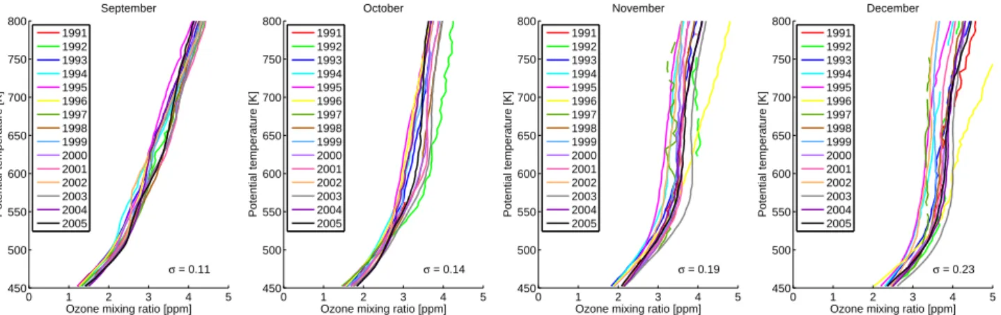
The interannual variability increases during the vortex for-mation period from September to December as illustrated in Fig. 1. Figure 1 shows monthly mean vertical profiles of ozone mixing ratios inside the polar vortex for each month from September to December and the years 1991–2005. The vortex is defined as the area north of 65◦_{N equivalent}

lat-itude here and the profiles are based on the ozone data set presented in the next section. The mean standard deviation of ozone mixing ratios between 500–700 K increases from 0.13 ppm in September to 0.24 ppm in December. To put these numbers into perspective: the highest standard devia-tions are observed in the polar vortex in winter (December to March) and are about 0.4 ppm.

(2)

0 1 2 3 4 5 450

500 550 600 650

σ = 0.11

Ozone mixing ratio [ppm]

Potential temperature [K]

1998 1999 2000 2001 2002 2003 2004 2005

0 1 2 3 4 5

450 500 550 600 650

σ = 0.14

1998 1999 2000 2001 2002 2003 2004 2005

0 1 2 3 4 5

450 500 550 600 650

σ = 0.19

1998 1999 2000 2001 2002 2003 2004 2005

0 1 2 3 4 5

450 500 550 600 650

σ = 0.23

1998 1999 2000 2001 2002 2003 2004 2005

Fig. 1.Monthly mean profiles of ozone mixing ratios in the polar vortex for the months from September to December and the years 1991–

2005. The vortex is defined as the area north of 65◦_{N equivalent latitude. Measurements are from satellites and ozone sondes (see text for}

details). The standard deviation of the monthly mean ozone mixing ratios in the vortex between 500–700 K is shown for every month in the lower right corner.

propagation of planetary scale waves from their source re-gions in the troposphere to the stratosphere (Charney and Drazin, 1961, see also Andrews et al., 1987, for a detailed re-view of middle atmosphere dynamics). Additionally, chem-ical processes lead to a strong meridional gradient in the ozone field at this time.

After autumnal equinox thermal emission leads to subsi-dence of air over the polar region and to a reversal of the circulation, westerly winds and eventually to the formation of the polar vortex (Schoeberl and Hartmann, 1991; Kawa et al., 2003). Then the strong westerlies surrounding the po-lar vortex again prevent the vertical propagation of planetary waves and suppress meridional mixing. But during the vor-tex formation period weak westerlies also permit waves with shorter wave lengths to propagate freely into the stratosphere and meridional mixing is enhanced. The meridional mixing introduces pronounced variability in the ozone abundance in high latitudes, which is later enclosed by the polar vortex. We show that the degree to which these waves transport low latitude air and ozone into the Arctic depends on the level of wave activity in the troposphere during this brief sensitive period, which typically lasts from the middle of September to the middle of November. In addition, we show that the lat-itudinal origin and the amount of subsidence the air experi-enced are correlated to the ozone amount enclosed in the vor-tex in early winter. This is in line with the general accepted mechanism that vortex ozone abundances are the result of a balance of mixing and subsidence and that the strength of both subsidence and mixing are determined by the amount of wave breaking in the stratosphere (Andrews et al., 1987). In a companion paper, we show that below a critical altitude (about 750 K), the chemical lifetime of ozone is long enough to let transport dominate over chemistry (Blessmann et al., 2012)

We examine the dynamical processes in autumn which lead to the observed variability in early winter on the basis of measured ozone data and model runs driven by ECMWF (European Centre for Medium Range Weather Forecasts) re-analyses. In Sect. 2, we present the ozone data set and the chemistry transport model used in this study. In Sect. 3, we show that the origin of air masses enclosed in the vortex and vortex mean ozone mixing ratios in early winter are related. For this, we use a set of artificial tracers, which are passively transported in the model and initialized in early autumn to values different from zero only in a limited spatial domain (see e.g. G¨unther et al., 2008). In Sect. 4, we show that the origin of air is related to the strength of the Brewer-Dobson circulation and meridional mixing. For this, we show correla-tions of the origin of air with the Eliassen-Palm flux through the midlatitudes in autumn. Finally, we show in Sect. 5 that EP flux and ozone are also related. Conclusions are given in Sect. 6.

Earlier studies show surprisingly high correlations be-tween late winter total ozone and early winter ozone mixing ratios (Kawa et al., 2005; Sinnhuber et al., 2006). E.g. the correlation between November ozone mixing ratios at 600 K from SBUV and March total ozone from TOMS is as high as 0.78 (Kawa et al., 2005). This is much higher than the direct effect expected if the variability of the partial column from 500–800 K in early winter would be conserved until late winter (Kawa et al., 2005). However, the causal relationships remain unclear and are not in the scope of this study.

2 Data and model

(3)

Fig. 2. Availability of ozone measurements from satellites and ozone sondes from 1991 to 2009.

2.1 Observational data

The observational data set includes measurements from ozone sondes and 7 satellite based instruments. Data is avail-able north of 30◦_{N from 1 August to 31 March for the time}

period 1991/1992 to 2008/2009.

All ozone measurements are binned and averaged in equiv-alent latitude bins with 5 degree resolution and in temporal bins with a resolution of 10 days. Equivalent latitude is cal-culated from data of the ECMWF ERA Interim reanalysis. Equivalent latitude is defined as the latitude an area enclosed by a potential vorticity contour would have, if it would be cir-cular and centered at the pole (e.g. Butchart and Remsberg, 1986). The vertical resolution of the data set is 5 K between 450 K and 1000 K.

The satellite measurements are from the solar occulta-tion instruments HALOE (Halogen Occultaocculta-tion Experiment) (Russell III et al., 1993), SAGE II & III (Stratospheric Aerosol and Gas Experiment) (McCormick et al., 1989), POAM II & III (Polar Ozone and Aerosol Measurement) (Lumpe et al., 1997, 2002) and ILAS I & II (Improved Limb Spectrometer) (Nakajima et al., 2004). Figure 2 shows the time periods where measurements are available from the in-dividual satellite instruments. No bias correction between the satellite instruments is applied, because potential instrumen-tal biases are much smaller than the interannual variability of ozone in the region studied here. All instruments cover the complete altitude range of the data set and have a vertical resolution of about 1–2 km.

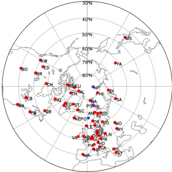
The ozone data set consists of around 14 000 ascents of ozone sondes from 55 stations, which are shown in Fig. 3. The measurements are checked manually for consistency and accuracy. After 2006, the data set is only based on ozone son-des. In the time periods where ozone sonde data and satellite

Fig. 3.Ozone sonde stations used in the ozone data set. Ships and

the ice drifting station NP-35 are shown in blue.

data overlap, ozone sondes and satellite instruments agree within 0.4 ppm.

2.2 Model

ATLAS is a global chemistry and transport model with a La-grangian (trajectory-based) transport and mixing scheme and stratospheric chemistry (Wohltmann and Rex, 2009; Wohlt-mann et al., 2010). Lagrangian models have several advan-tages over conventional Eulerian models, in particular no spurious numerical diffusion and a more realistic transport of conserved tracers.

We have based our model runs on ERA Interim reanalysis data (Dee et al., 2011) with a horizontal resolution of 2×2

degrees, 60 model levels and a temporal resolution of 6 h. Trajectories are integrated with a 30 min time step. The ver-tical coordinate is a hybrid coordinate, which is to a good approximation a potential temperature coordinate in the ver-tical domain used. Verver-tical motion is driven by ERA Interim heating rates (clear sky). The horizontal model resolution is 100 km and the model domain extends from 350 to 1500 K. The critical Lyapunov exponent, which adjusts the mixing strength, is set to 4 days−1_{, see Wohltmann and Rex (2009).}

(4)

−80 −60 −40 −20 0 20 40 60 80 400

500 600 700 800 900 1000 1100

Equivalent latitude [deg]

Fig. 4.Setup of the tracers at the start of the model run. The tracer

shown in Fig. 5 is highlighted.

A realistic transport of the tracers requires the reanalysis to contain a realistic representation of the observed Brewer-Dobson circulation. The ECMWF ERA Interim reanalysis has been shown to capture the basic features of the observed Brewer-Dobson circulation (Dee et al., 2011). In particular, the age of air is much more reasonable than in the preced-ing ECMWF ERA-40 reanalysis and within the error bars of observations (see Fig. 28 in Dee et al., 2011 or Legras and Fueglistaler, 2009). There are also some known discrepan-cies, like a too fast ascent at the tropics, but the ERA Interim data set is probably the best available reanalysis in the mo-ment.

2.3 Setup of the origin tracers

Artificial tracers of air mass origin have been used in the past to determine transport pathways in the atmosphere (e.g. G¨unther et al., 2008). Here, 117 tracers are initialized on 1 September in every year (1991/1992–2008/2009) to be able to calculate the origin of air masses enclosed in the vortex in early winter. The mixing ratio of each of these tracers is set to one inside a certain equivalent latitude interval and potential temperature interval and zero outside these intervals to iden-tify air masses from a certain spatial origin. Figure 4 shows the arrangement of tracers at the beginning of the model run. The tracers are initialized in a non-overlapping fashion, fill-ing the spatial domain of the model. The potential tempera-ture intervals start at 350 K in 100 K steps up to 950 K. The last three intervals are 950–1100 K, 1100–1300 K and 1300– 1500 K. The equivalent latitude intervals reach from 30◦_N

in 5 degree steps up to 90◦_{N. The first equivalent latitude}

in-terval is a special case and encloses the equivalent latitudes from 90◦_{S to 30}◦_N.

The tracers are transported and mixed down to lower val-ues than one in the course of the model run. This kind of

25 30 35 40 45 50 55 60 65 70 75 80 85 90 350

450 550 650 750

Equivalent latitude [deg]

Potential temperature [K] Mixing ratio [percent]

1 2 3 4 5

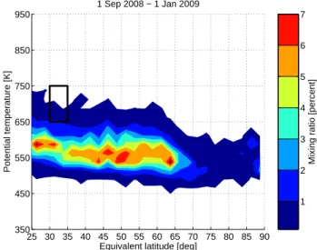
Fig. 5.Zonal mean tracer mixing ratio of a selected origin tracer

(30–35◦_{N equivalent latitude and 650–750 K) at the start of a model}

run (1 September 2008, the black box is the area of mixing ratios of 100 %) and in early winter (1 January 2009, filled contours).

tracer arrangement enables us to determine the origin of air by examining the fractions that the single tracers contribute to an air mass later in the model run. The fractions of the single tracers add up to one by definition at every model air parcel and can directly be interpreted as the percentage of air from a certain origin.

As an example, Fig. 5 shows the zonal mean tracer mixing ratios of a selected origin tracer (30–35◦_{N equivalent}

lati-tude and 650–750 K) at the start of a model run (1 September 2008) and in early winter (1 January 2009).

In the following, we will typically average over the tracer mixing ratios of all air parcels inside the polar vortex, which directly gives the fractions of air inside the vortex originating from a certain equivalent latitude and potential temperature interval on 1 September.

In some cases, it is also convenient to add up several trac-ers. E.g. to determine the fraction of air originating from equivalent latitudes south of 30◦_{N on 1 September, we add}

up all tracers south of 30◦_{N, i.e. the first column of tracers}

in Fig. 4.

3 Ozone and origin of air

Here we show that the origin of air masses and ozone mix-ing ratios in the vortex are related. As an example, Fig. 6 shows the time series of vortex mean ozone mixing ratios av-eraged over 525–575 K in early winter (30 December–8 Jan-uary, 1992 to 2009, black). The vortex is defined as the area north of 65◦_{N equivalent latitude here and in the subsequent}

(5)

19920 1994 1996 1998 2000 2002 2004 2006 2008 1

2 3 4 5

525−575 K Correlation 0.76

Year

1992 1994 1996 1998 2000 2002 2004 2006 2008 0

5 10 15 20 25 30 35 40

Fraction of air from 90 S − 30 N [percent]

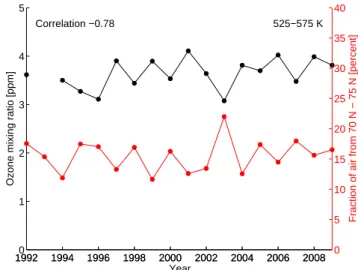
Fig. 6. Time series of vortex mean ozone mixing ratios at 525–

575 K in early winter (30 December–8 January, 1992–2009, black), superimposed by a time series of the fraction of air in the polar

vortex at 525–575 K which is originating south of 30◦_{N equivalent}

latitude on 1 September (red).

in the vortex in early winter at the same potential temper-ature level 525–575 K originating from equivalent latitudes south of 30◦_{N on 1 September (regardless of potential}

tem-perature on 1 September, red). This corresponds to the first column of tracers in Fig. 4. It can be seen that a high fraction of low latitude air masses is related to high ozone mixing ra-tios. Note that both time series show no significant trend and that the correlation is due to interannual variability. In par-ticular, there is no significant trend in ozone caused by the trend in ozone-depleting substances in the considered time period. The correlation coefficient of the detrended time se-ries is 0.76. Correspondingly, high ozone mixing ratios are related to a low fraction of air from high latitudes. Figure 7 shows the same ozone time series as before, but now the frac-tion of air originating from equivalent latitudes between 70– 75◦_{N. The correlation coefficient of the detrended time}

se-ries is−0.78.

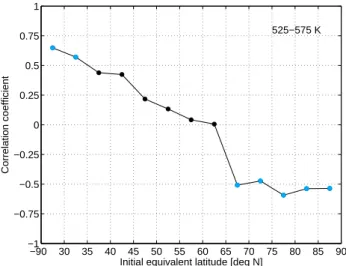
Figure 8 generalizes Figs. 6 and 7. The figure shows the correlation coefficients of the time series of vortex mean ozone mixing ratios in early winter at 525–575 K with sev-eral time series of origin tracers as a function of equivalent latitude. The time series of the origin tracers are the fraction of air in the vortex in early winter at 525–575 K originat-ing from the equivalent latitude interval given at the horizon-tal axis on 1 September. Correlations significant at the 95 % level are shown in blue. The time series are detrended in this figure and all following figures.

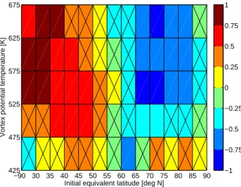
Figure 9 takes the generalization one step further. Each colored box shows the correlation coefficient of a time se-ries of vortex mean ozone mixing ratios in early winter and a time series of an origin tracer in early winter. The ozone time series is averaged over the potential temperature layers

19920 1994 1996 1998 2000 2002 2004 2006 2008 1

2 3 4 5

525−575 K Correlation −0.78

Year

1992 1994 1996 1998 2000 2002 2004 2006 2008 0

5 10 15 20 25 30 35 40

Fraction of air from 70 N − 75 N [percent]

Fig. 7. Time series of vortex mean ozone mixing ratios at 525–

575 K in early winter (30 December–8 January, 1992–2009, black), superimposed by a time series of the fraction of air in the polar

vortex at 525–575 K which is originating from 70–75◦_{N equivalent}

latitude on 1 September (red).

−90 30 35 40 45 50 55 60 65 70 75 80 85 90

−1 −0.75 −0.5 −0.25 0 0.25 0.5 0.75 1

525−575 K

Initial equivalent latitude [deg N]

Correlation coefficient

Fig. 8. Correlation of the origin of air inside the polar vortex

and vortex mean ozone mixing ratios at 525–575 K. Correlation of a time series (1992–2009) of vortex mean ozone mixing ratios in early winter at 525–575 K and a time series of the fraction of air in the vortex in early winter at 525–575 K originating from the equiv-alent latitude intervals given at the horizontal axis on 1 September. Correlation coefficients significant at the 95 % level are shown in blue. Time series are detrended.

(6)

−90 30 35 40 45 50 55 60 65 70 75 80 85 90 425

475 525 575

Vortex potential temperature [K]

−1 −0.75 −0.5 −0.25 0 0.25

Fig. 9.Correlation of the origin of air inside the polar vortex and

vortex mean ozone mixing ratios. Each colored box shows the cor-relation coefficient of a time series of vortex mean ozone mixing ratios in early winter and a time series of an origin tracer in early winter (1992–2009). The ozone time series is averaged over the po-tential temperature layers indicated at the vertical axis. The labels of the axis give the endpoints of the 50 K intervals. The time series of the origin tracer is the fraction of vortex air in early winter orig-inating from the equivalent latitude intervals given at the horizontal axis on 1 September and averaged over the potential temperature intervals given at the vertical axis. Correlation coefficients not sig-nificant at the 95 % level are crossed out. Time series are detrended.

and 575 K. Correlation coefficients not significant at the 95 % level are crossed out.

The figure shows that high positive correlation coefficients occur at low equivalent latitudes at most potential tempera-ture levels, which means that a high abundance of air from lower latitudes corresponds to high ozone mixing ratios in-side the polar vortex in all altitudes. Accordingly, a high amount of air masses from high latitudes corresponds to low ozone mixing ratios at most potential temperature levels.

Figure 10 shows the same data as Fig. 9, but now the ori-gin tracer is the fraction of vortex air in early winter origi-nating from a certain initial potential temperature interval on 1 September.

Note that we will use the term “net Lagrangian subsi-dence” in the following in the sense of the Lagrangian sub-sidence along the transport path of an air parcel between 1 September and early winter. This is different from the usual definition in the Transformed Eulerian Mean (TEM) sense at a fixed location in latitude and pressure (Andrews et al., 1987), which does not refer to the same air mass as time pro-ceeds. These two definitions can lead to very different results. The black line in Fig. 10 is the line of zero Lagrangian sub-sidence. The positive correlation coefficients near the line of zero Lagrangian subsidence (for vortex potential temperature levels near the initial potential temperature levels) indicate that higher vortex mean ozone mixing ratios in early winter

350 450 550 650 750 850 950 1100 425

475 525 575

Initial potential temperature [K]

−1 −0.75 −0.5 −0.25 0 0.25

Fig. 10.Same as Fig. 9, but now the origin tracer is the fraction of

vortex air in early winter originating from the potential temperature interval given at the horizontal axis on 1 September. Correlation coefficients not significant at the 95 % level are crossed out. The black line is the line of zero Lagrangian subsidence. Time series are detrended.

are typically correlated with a higher abundance of air from lower initial potential temperature levels on 1 September (re-spectively with less net Lagrangian subsidence). At first, that seems to be in contradiction to the typical increase of ozone mixing ratios with potential temperature.

However, an origin from a certain potential temperature level is also correlated with a preferred latitudinal origin, which is shown in Fig. 11. The figure shows a scatter plot of the vortex mean of two origin tracers in early winter at 525– 575 K. Each marker gives the values of the two tracers in the particular year shown inside the marker. The tracer on the horizontal axis is the fraction of air originating from equiv-alent latitudes south of 30◦_{N on 1 September. The tracer on}

the vertical axis is the fraction of air originating from the ini-tial potenini-tial temperature interval 550–650 K on 1 September (i.e. with a maximum of 125 K Lagrangian subsidence).

Figure 11 indicates that an origin in southern or tropical latitudes is typically correlated with less net Lagrangian sub-sidence (lower initial potential temperatures) than an origin in higher latitudes. This is consistent with ascent (in the TEM sense) in the tropics and subsidence (in the TEM sense) in polar regions, as expected from the Brewer-Dobson circula-tion: on average, air will spent more time in low latitudes if it originates in low latitudes, and hence more time in regions with upwelling or weak downwelling. Since ozone mixing ratios are higher at the same potential temperature level in the tropics than in the polar regions in the considered altitude range, less Lagrangian subsidence is correlated with higher ozone mixing ratios.

(7)

0 2 4 6 8 10 12 14 16 18 0

1 2 3 4 5 6 7 8 9 10

92

93

94 95

96

97

98

99

00

01

02

03

04

05 06

07 08

09

Percentage of air from <30 deg N

Percentage of air from 550−650 K on 1 Sep

Correlation 0.82

525−575 K

Fig. 11.Scatter plot of the vortex mean of two origin tracers in early

winter at 525–575 K. Each marker gives the values of the two trac-ers in the particular year shown inside the marker. The tracer on the horizontal axis is the fraction of air originating from equivalent

lati-tudes south of 30◦_{N on 1 September. The tracer on the vertical axis}

is the fraction of air originating from the initial potential tempera-ture interval 550–650 K on 1 September (i.e. with a maximum of 125 K Lagrangian subsidence).

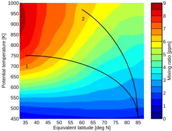
a function of potential temperature and equivalent latitude. Pathway 1 shows the situation in years with a high fraction of air from low latitudes enclosed in the vortex, which is typ-ically also connected with low net Lagrangian subsidence. Due to the mean ozone distribution, this leads to relatively high ozone values in the vortex. This situation should also typically be connected to a strong Brewer-Dobson circula-tion, enhanced meridional mixing and a high EP flux through the tropopause (Andrews et al., 1987). We will show the re-lationship between EP flux and origin of air (respectively ozone) in more detail in the next sections. The correlation between EP flux and ozone (but not origin of air) has already been the subject of many studies (e.g. Fusco and Salby, 1999; Weber et al., 2003). Note that low net Lagrangian subsidence is connected here to a strong Brewer-Dobson circulation, and hence, a high subsidence in the TEM sense in high latitudes. This is no contradiction as long as the air spends not too much time in the region of high subsidence.

Pathway 2 shows the situation in years with a low frac-tion of air from low latitudes enclosed in the vortex, which is typically connected with high Lagrangian subsidence, low ozone and a weak Brewer-Dobson circulation.

4 EP flux and origin of air

The divergence of the EP flux is a measure for the momen-tum deposited in the middle atmosphere by breaking waves that are propagating from the troposphere to the stratosphere

35 40 45 50 55 60 65 70 75 80 85

450 500 550 600 650 700 750 800 850 900 950 1000

1

2

Equivalent latitude [deg N]

Mixing ratio [ppm]

0 1 2 3 4 5 6 7 8 9

Fig. 12.Schematical illustration of the pathway of air in two years

with extreme conditions. Colors show the mean ozone distribution in September. Pathway 1 shows the situation in years with a high fraction of air from low latitudes enclosed in the vortex, which is typically also connected with low net Lagrangian subsidence. Due to the mean ozone distribution, this leads to relatively high ozone values in the vortex. This situation is also typically connected with a strong Brewer-Dobson circulation and a high EP flux through the tropopause. Pathway 2 shows the situation in years with a low frac-tion of air from low latitudes enclosed in the vortex, which is typ-ically connected with high net Lagrangian subsidence, low ozone and a weak Brewer-Dobson circulation.

(e.g. Andrews et al., 1987). Both the strength of the zonal mean residual circulation and of meridional mixing are re-lated to the amount of momentum deposited in the strato-sphere (Andrews et al., 1987). The residual circulation be-low a given pressure level can only be influenced by waves breaking above this level (downward control principle, see Haynes et al., 1991). EP flux enters the stratosphere mainly through the mid-latitude tropopause. The EP flux in autumn for a given pressure level is given here as the vertical com-ponent of the flux through this level averaged over 45–75◦_N

and from September to November. This equals in good ap-proximation the overall divergence above this level in au-tumn. Each potential temperature layer in our analysis is as-signed a pressure level by averaging over the pressure in the layer. EP flux is used intentionally here as a single-valued proxy for complicated dynamical processes and to show up the basic relationships.

(8)

−90 30 35 40 45 50 55 60 65 70 75 80 85 90 −1

−0.75 −0.5 −0.25 0 0.25

EP flux through mid latitudes in autumn. Correlation of a time se-ries (1992–2009) of the vertical component of the EP flux through

a pressure level equivalent to 525–575 K averaged over 45–75◦_N

and from September to November and a time series of the frac-tion of air in the vortex in early winter at 525–575 K originating from the equivalent latitude intervals given at the horizontal axis on 1 September. Correlation coefficients significant at the 95 % level are shown in blue. Time series are detrended.

expected by the mechanisms of the Brewer-Dobson circula-tion.

Figure 14 again generalizes Fig. 13. Now, each colored box shows the correlation coefficient of a time series of EP flux through a layer in autumn and a time series of an origin tracer at this layer in early winter. The time series of the origin tracer is the fraction of vortex air in early win-ter originating from the equivalent latitude inwin-tervals given at the horizontal axis on 1 September and averaged over the potential temperature intervals given at the vertical axis, in the same manner as in Fig. 9. The EP flux is calculated for the potential temperature layers at the vertical axis, but is no function of the horizontal axis.

The figure shows that high amounts of air masses from lower latitudes are correlated with enhanced EP flux at all altitude levels and that high amounts of air masses from high latitudes are anti-correlated with the EP flux.

There is some sensitivity with respect to the averaging pe-riod of the EP flux in the correlations. Correlations are best for September to November, which most closely matches the period with enhanced meridional mixing. Both the peri-ods September to October and September to December show lower correlations.

5 EP flux and ozone

If both vortex mean ozone in early winter and EP flux in autumn correlate with the origin of air, it is to be expected

−90 30 35 40 45 50 55 60 65 70 75 80 85 90 425

475 525 575

−1 −0.75 −0.5 −0.25 0 0.25

EP flux through mid latitudes in autumn. Each colored box shows the correlation coefficient of a time series of EP flux through a layer in autumn and a time series of an origin tracer in early winter at the same layer (1992–2009). The EP flux time series is the vertical component of the flux through the layer given at the vertical axis

av-eraged over 45–75◦_{N and from September to November. The}

ori-gin tracer is the fraction of vortex air in early winter oriori-ginating from the equivalent latitude intervals given at the horizontal axis on 1 September and averaged over the potential temperature intervals given at the vertical axis. Correlation coefficients not significant at the 95 % level are crossed out. Time series are detrended.

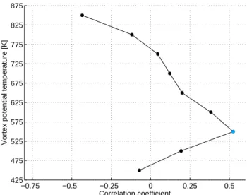
that also ozone and EP flux correlate with each other, as al-ready shown for other cases by several studies (e.g. Fusco and Salby, 1999; Weber et al., 2003). Figure 15 shows the correlation between vortex mean ozone mixing ratios in early winter at a particular level and the EP flux in autumn through this level (all quantities are defined as in the last sections). While the correlations are not as high as in the other plots, there is a positive correlation between EP flux and ozone mixing ratio at the layers 525–575 K and 575–625 K (with a significance of 97 % and 86 %, respectively).

(9)

−0.75 −0.5 −0.25 0 0.25 0.5 425

475 525 575 625 675 725 775 825 875

Fig. 15.Correlation of EP flux through mid latitudes in autumn and

vortex mean ozone mixing ratios in early winter. The EP flux time series is the vertical component of the flux through the layer given

at the vertical axis averaged over 45–75◦_{N and from September to}

November. The ozone time series is the vortex mean ozone mix-ing ratio in early winter at the given layer. Correlation coefficients significant at the 95 % level are shown in blue. Time series are de-trended.

6 Conclusions

We have used model runs of the ATLAS CTM in conjunc-tion with a comprehensive ozone dataset based on sondes and satellites to deduce statistical relationships between the ozone amount in the polar vortex in early winter and the lat-itudinal and vertical origin of air in September. For this, we used a set of artificial model tracers of air mass origin ini-tialized in September and transported with the model until early January, when the distributions of the tracers were cor-related with the ozone amount in the vortex. In addition, we examined the relationship between the wave activity in au-tumn (represented by the EP flux through the mid-latitude tropopause from September to November) and both the ori-gin of air and the ozone amount in the early winter polar vortex. Our main findings are:

– Both high wave activity and high ozone are connected to a large fraction of vortex air originating from low lat-itudes at the beginning of autumn. This air has typically experienced relatively small net subsidence (in a La-grangian sense) in autumn.

– High wave activity during polar vortex formation in au-tumn leads to high mixing ratios of ozone enclosed into the vortex at the beginning of winter (and vice versa). This is in line with earlier results for other seasons (e.g. Fusco and Salby, 1999) and with expectations from basic mechanisms of the Brewer-Dobson circulation (e.g. Andrews

et al., 1987). The relationships between air mass origin and EP flux or ozone have not been examined in detail so far for the autumn season to our knowledge. The use of the artificial origin tracers (e.g. G¨unther et al., 2008) enables a direct and intuitive study of the origin of air masses, which is not pos-sible with indirect methods like the measurement of chemi-cally conserved species.

Our study qualitatively confirms the results of Rosenfield and Schoeberl (2001). Rosenfield and Schoeberl (2001) show that in each year, there are two populations of air parcels end-ing up in the vortex: air parcels that experience high subsi-dence and often originate from the upper stratosphere and mesosphere, and air parcels that experience low subsidence and typically originate from more southern latitudes. These populations contribute different fractions of the air parcels in the vortex in different years, which causes interannual vari-ability in conserved tracers. There are also indications in this study that dynamically more active years have a greater con-tribution from the population with low descent rates.

In a companion paper, we show that below a critical al-titude (about 750 K), the chemical lifetime of ozone is long enough to let transport dominate over chemistry (Blessmann et al., 2012).

Acknowledgements. We thank ECMWF for providing reanalysis data and all PIs for providing ozone sonde data. Work at AWI was partially supported by the EC project RECONCILE, Grant Agreement No. 236365.

Edited by: M. Dameris

References

Andrews, D. G., Holton, J. R., and Leovy, C. B.: Middle Atmo-sphere Dynamics, Academic Press, 1987.

Blessmann, D., Wohltmann, I., Lehmann, R., and Rex, M.: Persis-tence of ozone anomalies in the Arctic stratospheric vortex in autumn, Atmos. Chem. Phys., 12, 4817–4823, doi:10.5194/acp-12-4817-2012, 2012.

Butchart, N. and Remsberg, E. E.: The area of the stratospheric po-lar vortex as a diagnostic for tracer transport on an isentropic surface, J. Atmos. Sci., 43, 1319–1339, 1986.

Charney, J. G. and Drazin, P. G.: Propagation of planetary-scale dis-turbances from the lower into the upper atmosphere, J. Geophys. Res., 66, 83–109, 1961.

(10)

Frieler, K., Rex, M., Salawitch, R. J., Canty, T., Streibel, M., Stimpfle, R. M., Pfeilsticker, K., Dorf, M., Weisenstein, D. K., and Godin-Beekmann, S.: Toward a better quantitative under-standing of polar stratospheric ozone loss, Geophys. Res. Lett., 33, L10812, doi:10.1029/2005GL025466, 2006.

Fusco, A. C. and Salby, M. L.: Interannual variations of total ozone and their relationship to variations of planetary wave activity, J. Climate, 12, 1619–1629, 1999.

G¨unther, G., M¨uller, R., von Hobe, M., Stroh, F., Konopka, P., and Volk, C. M.: Quantification of transport across the boundary of the lower stratospheric vortex during Arctic winter 2002/2003, Atmos. Chem. Phys., 8, 3655–3670, doi:10.5194/acp-8-3655-2008, 2008.

Haynes, P. H., Marks, C. J., McIntyre, M. E., Shepherd, T. G., and Shine, K. P.: On the “downward control” of extratropical diabatic circulations by eddy-induced mean zonal forces, J. Atmos. Sci., 48, 651–678, 1991.

Kawa, S. R., Bevilacqua, R. M., Margitan, J. J., Douglass, A. R., Schoeberl, M. R., Hoppel, K. W., and Sen, B.: Interaction be-tween dynamics and chemistry of ozone in the setup phase of the Northern Hemisphere polar vortex, J. Geophys. Res., 108, 8310, doi:10.1029/2001JD001527, 2003.

Kawa, S. R., Newman, P. A., Stolarski, R. S., and Bevilacqua, R. M.: Fall vortex ozone as a predictor of springtime total ozone at high northern latitudes, Atmos. Chem. Phys., 5, 1655–1663, doi:10.5194/acp-5-1655-2005, 2005.

Legras, B. and Fueglistaler, S.: Age of air and heating rates: compar-ison of ERA-40 with ERA-Interim, presentation at EGU General Assembly, Vienna, 2009.

Lumpe, J. D., Bevilacqua, R. M., Hoppel, K. W., Krigman, S. S., Kriebel, D. L., Debrestian, D. J., Randall, C. E., Rusch, D. W., Brogniez, C., Ramananah´erisoa, R., Shettle, E. P., Olivero, J. J., Lenoble, J., and Pruvost, P.: POAM II retrieval algorithm and error analysis, J. Geophys. Res., 102, 23593–23614, 1997. Lumpe, J. D., Bevilacqua, R. M., Hoppel, K. W., and Randall, C. E.:

POAM III retrieval algorithm and error analysis, J. Geophys. Res., 107, 4575, doi:10.1029/2002JD002137, 2002.

satellite, Proc. SPIE, 5571, 293–300, 2004.

Rosenfield, J. E. and Schoeberl, M. R.: On the origin of polar vortex air, J. Geophys. Res., 106, 33485–33497, 2001.

Russell III, J. M., Gordey, L. L., Park, J. H., Drayson, S. R., Hes-keth, D. H., Cicerone, R. J., Tuck, A. F., Frederick, J. E., Harries, J. E., and Crutzen, P.: The Halogen Occultation Experiment, J. Geophys. Res., 98, 10777–10797, 1993.

Schoeberl, M. R. and Hartmann, D. L.: The dynamics of the strato-spheric polar vortex and its relation to springtime ozone deple-tions, Science, 251, 46–52, 1991.

Sinnhuber, B.-M., von der Gathen, P., Sinnhuber, M., Rex, M., K¨onig-Langlo, G., and Oltmans, S. J.: Large decadal scale changes of polar ozone suggest solar influence, Atmos. Chem. Phys., 6, 1835–1841, doi:10.5194/acp-6-1835-2006, 2006. Tilmes, S., M¨uller, R., Grooß, J.-U., Nakajima, H., and Sasano, Y.:

Development of tracer relations and chemical ozone loss dur-ing the setup phase of the polar vortex, J. Geophys. Res., 111, D24S90, doi:10.1029/2005JD006726, 2006.

Weber, M., Dhomse, S., Wittrock, F., Richter, A., Sinnhuber, B.-M., and Burrows, J. P.: Dynamical control of NH and SH win-ter/spring total ozone from GOME observations in 1995–2002, Geophys. Res. Lett., 30, 1583, doi:10.1029/2002GL016799, 2003.

WMO: World Meteorological Organization (WMO)/United Na-tions Environment Programme (UNEP), Scientific assessment of ozone depletion: 2010, Global Ozone Research and Monitoring Project – Report No. 52, 2011.

Wohltmann, I. and Rex, M.: The Lagrangian chemistry and trans-port model ATLAS: validation of advective transtrans-port and mixing, Geosci. Model Dev., 2, 153–173, doi:10.5194/gmd-2-153-2009, 2009.