On reconstruction of time series in climatology

(1)

CPD

11, 4701–4728, 2015

On reconstruction of time series in

climatology

V. Privalsky and A. Gluhovsky

Title Page

Abstract Introduction

Conclusions References

Tables Figures

◭ ◮

Back Close

Full Screen / Esc

Printer-friendly Version Interactive Discussion

Discussion

P

a

per

|

Discussion

P

a

per

|

Discussion

P

a

per

|

Discussion

P

a

per

|

Clim. Past Discuss., 11, 4701–4728, 2015 www.clim-past-discuss.net/11/4701/2015/ doi:10.5194/cpd-11-4701-2015

This discussion paper is/has been under review for the journal Climate of the Past (CP). Please refer to the corresponding final paper in CP if available.

On reconstruction of time series in

climatology

V. Privalsky1and A. Gluhovsky2

1

Space Dynamics Laboratory (ret.), VEP Consulting, Logan, Utah, USA

2

Department of Earth, Atmospheric, and Planetary Sciences and Department of Statistics, Purdue University, West Lafayette, Indiana, USA

Received: 28 July 2015 – Accepted: 1 September 2015 – Published: 6 October 2015

Correspondence to: V. Privalsky (vprivalsky@gmail.com)

Published by Copernicus Publications on behalf of the European Geosciences Union.

(2)

CPD

11, 4701–4728, 2015

climatology

Title Page

Tables Figures

◭ ◮

Back Close

Full Screen / Esc

Discussion

P

a

per

|

Discussion

P

a

per

|

Discussion

P

a

per

|

Discussion

P

a

per

|

Abstract

The approach to time series reconstruction in climatology based upon cross-correlation coefficients and regression equations is mathematically incorrect because it ignores the dependence of time series upon their past. The proper method described here for the bivariate case requires the autoregressive time- and frequency domains

model-5

ing of the time series which contains simultaneous observations of both scalar series with subsequent application of the model to restore the shorter one into the past. The method presents further development of previous efforts taken by a number of authors starting from A. Douglass who introduced some concepts of time series analysis into paleoclimatology. The method is applied to the monthly data of total solar irradiance

10

(TSI), 1979–2014, and sunspot numbers (SSN), 1749–2014, to restore the TSI data over 1749–1978. The results of the reconstruction are in statistical agreement with observations.

1 Introduction

An important task in climatology and paleoclimatology consists in the reconstruction of

15

a time series of some variable over the time interval when that variable was not mea-sured. This task is solved by using proxy data – observations of a different variable, or variables supposed to be closely related to the variable of interest during the time interval of interest. A typical example would be restoring the annual surface tempera-ture over the past centuries using dendrochronology data – time series of annual tree

20

ring widths within the geographical area of interest. The observation data over the time interval when both variables (tree rings as the proxy and temperature as the variable to be restored) have been properly measured, are analysed and the relation between them is used to reconstruct the temperature time series into a more or less distant past, depending on the amount of tree rings observations. Quite often, the

mathemat-25

(3)

CPD

11, 4701–4728, 2015

climatology

Title Page

Tables Figures

◭ ◮

Back Close

Full Screen / Esc

Discussion

P

a

per

|

Discussion

P

a

per

|

Discussion

P

a

per

|

Discussion

P

a

per

|

the cross-correlation coefficient between the time series of the proxy variable and the variable that is being reconstructed on the basis of the available simultaneous observa-tions is high, a regression equation is built and the missing past values of temperature are reconstructed on the basis of that equation. This is how it is done both in the sim-plest bivariate case (a proxy and the variable to be restored) and in the multivariate

5

case when the variable of interest is reconstructed on the basis of a multivariate linear regression equation (e.g., Bradley, 2015; Santos et al., 2015). The variables can be transformed in some way before the reconstruction (for example, time series of princi-pal components of expansions into empirical orthogonal functions are used instead of the original data, see Tingley et al., 2012) but the general principle remains the same:

10

build a regression equation.

Yet, this cross-correlation/regression approach is generally not correct for analysing multivariate time series. Their statistical properties cannot be understood and the miss-ing past data should not be reconstructed without a more sophisticated analysis than just through cross-correlation coefficients and regression equations. The key factor

15

that makes time series behave in a more complicated manner is their dependence upon time and, consequently, upon frequency, which does not exist in the case of ran-dom variables for which a cross-correlation coefficient and a regression equation are exhaustive. Generally, consecutive values of time series depend upon their past and the relationship between the scalar components of a multivariate time series depends

20

upon past values of all of its components. The time domain properties define the time series’ properties in the frequency domain, and their study allows one to obtain addi-tional information about relations between the scalar components of a multivariate time series.

The goals of this study are to show how to

25

– analyze a multivariate time series in time and frequency domains to obtain and interpret the information necessary for reconstructing one of the time series’ com-ponents into the past and

(4)

CPD

11, 4701–4728, 2015

climatology

Title Page

Tables Figures

◭ ◮

Back Close

Full Screen / Esc

Discussion

P

a

per

|

Discussion

P

a

per

|

Discussion

P

a

per

|

Discussion

P

a

per

|

– apply the results of this analysis to reconstruct past values of the time series on the basis of observations made during a relatively short and recent time interval.

Section 2 contains some historical notes, Sect. 3 describes the mathematical ap-proach used in the paper; it is based upon autoregressive time- and frequency do-mains analysis of multivariate (in our case, bivariate) time series. Section 4 provides

5

an example with actual bivariate data (the data description and steps to be taken to reconstruct the time series). The methodology and results are summed up in Sect. 5, which also contains some practical recommendations.

2 Historical notes

Seemingly the first effort to reconstruct a climatic time series was made by the founder

10

of the science of dendrochronology A. Douglass who suggested “a mathematical for-mula for calculating the growth of trees when the rainfall is known” and vice versa (Douglass, 1919). His studies of tree rings growth and climate dependence upon each other and upon sunspot numbers include important achievements such as

– discovering and analyzing dependence between time series of tree-rings growth

15

and sunspot numbers (Douglass, 1909, p. 228; Douglass, 1928),

– suggesting an extended memory (autoregressive) type of model for the time se-ries of precipitation (1919, p. 68),

– regarding the sunspot – tree rings system as inertial (Douglass, 1936),

– noting that the correlation coefficient may not properly reflect the dependence

20

between time series (“The similarity between two trees curves . . . is only partly expressed by a correlation coe_fficient.” Douglass, 1936, p. 29),

(5)

CPD

11, 4701–4728, 2015

climatology

Title Page

Tables Figures

◭ ◮

Back Close

Full Screen / Esc

Discussion

P

a

per

|

Discussion

P

a

per

|

Discussion

P

a

per

|

Discussion

P

a

per

|

The first analyses that take into account the behavior of time series of climate and tree-rings in both time and frequency domains through correlation functions, spectra, and coherence functions and describe the response of tree-growths to climatic factors were conducted by Fritts (1976). Concepts of response functions “to describe the tree-ring response to variation in climate” and transfer function, “which transforms values of

5

ring width into estimates of climate. . . ”, were also introduced, adverse effects of filtering noted but no explicit time- or frequency domains models was suggested. A frequency domain description of tree-ring and climate data through coherence function estimates was also given by Guiot (1982).

Probably, the first example of building an explicit time-domain model was presented

10

by Guiot (1985) who used a set of “mutually exclusive” linear filters to split the en-tire frequency range of the data into separate frequency bands, obtained a regression equation for each band and then combined them into a single time-domain equation connecting temperature to tree-rings.

Guiot (1986) introduced the concept of parametric time domain models into

paleo-15

climatology and used scalar ARMA models and/or regression equation to estimate the transfer function. The reconstruction quality was estimated on the basis of correlation coefficients with an “optimal” proxy data set.

More efforts were undertaken later to apply methods of time series analysis in pale-oclimatology, including the use of the Kalman filter (Visser and Molenaar, 1988) as well

20

as applications of the Bayesian approach to climate reconstruction (e.g., von Storch et al., 2004; Hasslett et al., 2006; Tingley and Hubert, 2010).

Though the correlation/regression approach still seems to prevail in paleoclimatol-ogy, our approach based upon an explicit time-domain model of the tree-rings–climate system in the form of a bivariate stochastic difference equation including system’s

de-25

scription in the frequency domain should be regarded as an improvement of methods suggested by previous authors starting from the founder of dendrochronology A. Dou-glass.

(6)

CPD

11, 4701–4728, 2015

climatology

Title Page

Tables Figures

◭ ◮

Back Close

Full Screen / Esc

Discussion

P

a

per

|

Discussion

P

a

per

|

Discussion

P

a

per

|

Discussion

P

a

per

|

3 Data analysis tools

The basic difference between random variables and random functions had been re-vealed almost 60 years ago in the classical work by Gelfand and Yaglom (1957). They proved, in particular, that the amount of information about a (Gaussian) random vari-able x1 contained in another (Gaussian) random variable x2 is J=−12log(1−r

2 12),

5

wherer12 is the correlation coefficient between the variables. According to their fun-damental results, the respective information quantity – the average information rate per unit time – for discrete stationary random functionsx1,nandx2,nis

i(x1,n,x2,n)= f_N

Z

0

logh1−γ₁₂2 (f)idf,

where γ₁₂2 (f) is the coherence squared function (see below), f is the frequency,

10

fN=1/2∆t is the Nyquist frequency, and ∆t is the sampling interval. Thus, the

de-pendence between time series is described with a function of frequency and is not associated with the cross-correlation coefficient. In other words, the cross-correlation coefficient cannot characterize relations between the components of a multivariate time series. The coherence function was used in paleoclimatology by Fritts (1976) and other

15

authors (see Sect. 2) at the time when the time series analysis has already become a well-developed science but the Douglass’ remark regarding the inadequacy of the correlation coefficient for time series analysis made as early as in 1936 looks quite visionary.

Monographs and papers on methods of multiple time series analysis including

esti-20

(7)

CPD

11, 4701–4728, 2015

climatology

Title Page

Tables Figures

◭ ◮

Back Close

Full Screen / Esc

Discussion

P

a

per

|

Discussion

P

a

per

|

Discussion

P

a

per

|

Discussion

P

a

per

|

Consider now how the linear regression model

x1=ϕx2+a, (1)

wherex1,x2, andaare zero mean random variables, should change in the case of a bi-variate zero mean time seriesx_n=[x1,n,x2,n]′(the strike denotes matrix transposition).

For the time seriesx_n,n=1, 2,. . ., one should expect that its scalar componentsx1,n

5

andx2,ndepend upon their own past values and, possibly, upon the past values of the

other component. This means that the linear regression Eq. (1) would be transformed into a system of linear stochastic difference equations

x1,n=ϕ

(1)

11x1,n−1+ϕ (1)

12x2,n−1+. . .+ϕ (p)

11x1,n−p+ϕ (p)

12x2,n−p+a1,n (2)

x2,n=ϕ

(1)

21x1,n−1+ϕ (1)

22x2,n−1+. . .+ϕ (p)

21x1,n−p+ϕ (p)

22x2,n−p+a2,n.

10

which presents a generalization of the regression Eq. (1) to the case of bivariate time series. Herea_1,_n and a_2,_n are white noise innovation sequences (time series analogs of the regression error a in Eq. 1), the coefficients ϕ(₁₁i), ϕ₂₂(i),i =1,. . .,p define the dependence ofx1,nandx2,nupon their own past values,ϕ

(i) 12,ϕ

(i)

21, i=1,. . .,pdescribe the connection betweenx1,n andx2,n, and the integer parameter pis the largest time

15

lag, at which any of the coe_fficientsϕ(_{i j}i)in Eq. (2) is statistically di_fferent from zero. In a matrix form, Eq. (2) is written as

x_n=

p

X

j=1

Φ_j_x_n₋_j₊_a_n_, ₍₃₎

where

Φ_j₌

"

ϕ(₁₁j) ϕ(₁₂j) ϕ(₂₁j) ϕ(₂₂j) #

(4)

20

(8)

CPD

11, 4701–4728, 2015

climatology

Title Page

Tables Figures

◭ ◮

Back Close

Full Screen / Esc

Discussion

P

a

per

|

Discussion

P

a

per

|

Discussion

P

a

per

|

Discussion

P

a

per

|

anda_n=[a1,n,a2,n]′.

The stochastic di_fference Eq. (2) (or its matrix form Eq. 3) is a bivariate autoregres-sive model of orderp[notation: AR(p)] and its innovation sequence covariance matrix is

Ra=

R11 R12

R21 R22

. (5)

5

It is important to note that the AR model has appeared here not because it had been used in the classical monograph by Box and Jenkins (1970) or anywhere else but because it followed directly from the desire to properly describe the linear connection between two scalar time series.

The properties of the time seriesx_nin the frequency domain are described with the

10

spectral matrix

s(f)=

s11(f) s12(f)

s21(f) s22(f)

, (6)

which is obtained through a Fourier transform of Eq. (3). Here,s11(f), s22(f) are the spectra ands₁₂(f),s₂₁(f) are the complex-conjugated cross-spectra of the time series

x1,nandx2,n.

15

In particular, the coherence squared function is found from the matrix Eq. (6) as

γ2 12(f)=

|s₁₂(f)|2

s11(f)s22(f)

(7)

(e.g., Bendat and Piersol, 2010).

The coherence function γ₁₂(f), which satisfies the condition 0≤γ₁₂(f)≤1, can be regarded as a frequency-dependent “cross-correlation coefficient” between the

compo-20

(9)

CPD

11, 4701–4728, 2015

climatology

V. Privalsky and A. Gluhovsky Title Page Abstract Introduction Conclusions References Tables Figures ◭ ◮ ◭ ◮ Back Close

Full Screen / Esc

Printer-friendly Version Interactive Discussion Discussion P a per | Discussion P a per | Discussion P a per | Discussion P a per |

coefficient that defines the degree of linear dependence between the components of a bivarite time series.

Other functions of frequency that describe relations between time series, such as coherent spectra and frequency response functions (e.g., Bendat and Piersol, 2010), will not be used in this article.

5

The time domain model Eq. (3) is also valid for M-variate time series x_n= [x_1,_n,. . .,x_M_,_n]′; in this general case, the matrix AR coefficients

Φ_j₌

     

ϕ₁₁(j) ϕ₁₂(j) . . . ϕ(₁j_M) ϕ₂₁(j) ϕ₂₂(j) . . . ϕ(₂j_M)

..

. ... ...

ϕ_M(j)₁ ϕ_M(j)₂ . . . ϕ(_MMj)       . (8)

The innovations sequence of an M-variate time series is a_n₌[a1,n,. . .,aM,n]′ and its

covariance matrix takes the form

10

R_a=



   

R11 R12 . . . R1M

R21 R22 . . . R2M

..

. ... ...

R_M1 RM2 . . . RMM

     . (9)

The spectral matrix Eq. (6) changes to

s(f)=



   

s11(f) s12(f) . . . s1M(f)

s21(f) s22(f) . . . s2M(f)

..

. ... ...

s_M1(f) sM2(f) . . . sMM(f)

     , (10)

withs_{i j}(f) being the spectral (ifi =j) and cross-spectral (ifi 6=j) densities, respectively, of the time series xi,n,i =1,. . .,M. The spectral matrix Eq. (10) is used to calculate

15

(10)

CPD

11, 4701–4728, 2015

climatology

Title Page

Tables Figures

◭ ◮

Back Close

Full Screen / Esc

Discussion

P

a

per

|

Discussion

P

a

per

|

Discussion

P

a

per

|

Discussion

P

a

per

|

other spectral functions such as multiple and partial coherences, coherent spectra, etc. (see Bendat and Piersol, 2010).

The task of fitting a proper autoregressive model to a bivariate time series is dis-cussed, for example, in Box et al. (2015), while some recommendations for the case of climate data analysis can be found in Privalsky (2015). A key point in the parametric

5

time series analysis is choosing a proper order p for the model Eq. (3); the recom-mended approach is to do it with the help of order-selection criteria: Akaike’s AIC, Schwarz–Rissanen’s BIC, Parzen’s CAT, and Hannan–Quinn’sϕ(e.g., Parzen, 1977; Hannan and Quinn, 1979; Box et al., 2015).

4 An example of a bivariate time series reconstruction

10

The following example with actual observations – sunspot numbers and total solar ir-radiance of the Earth – demonstrates, among other things, that the linear regression approach to reconstructing past data is generally not correct. Specifically, it would not be proper to reconstruct past valuesx1,n,n=1,. . .,N1 of any scalar time series x1,n

known over the interval [N1+1,N2] using the linear regression between x1,n and

an-15

other scalar time series x_2,_n known atn=1,. . .,N₁,. . .,N₂. This general statement is true as long as the modulus of the cross-correlation coefficient betweenx1,n andx2,n

calculated for the interval [N1+1,N2] is not equal to 1. Note that though the depen-dence between time series at the input and output of any linear filter is, of course, strictly linear, the cross-correlation coefficient between them is always less than 1.

20

(11)

CPD

11, 4701–4728, 2015

climatology

Title Page

Tables Figures

◭ ◮

Back Close

Full Screen / Esc

Discussion

P

a

per

|

Discussion

P

a

per

|

Discussion

P

a

per

|

Discussion

P

a

per

|

4.1 Data and data analysis

Consider the task of restoring past values of the total solar irradiance (TSI) x1,n on

the basis of its connection to the time series of sunspot numbers (SSN) x2,n. The

time series of monthly TSI values is available at the KNMI site http://climexp.knmi.nl/ selectindex.cgi (also, see Fröhlich, 2000) while the latest set of SSN data (version 2.0)

5

is taken from the site of the Solar Influences Data Analysis Center (see http://sidc.oma. be/). A detailed description of this new time series can be found in Clette et al. (2014). We use observation data forx1,n and for x2,n from 1979 through 2014 and from 1749

through 2014, respectively, at the sampling rate∆t=1 month (N1=2760,N2=3192). The values of TSI and SSN over the 432-month long common interval of observations

10

fromN1+1 throughN2are shown in Fig. 1.

Both processes are dominated by the 11 year cycle but also show variability at smaller time scales. The autoregressive estimates of the TSI and SSN spectra are shown in Fig. 2. The optimal AR orders for the scalar time series models arep=32 and p=33, respectively. The spectra contain strong peaks at the frequency fs≈

15

0.091 year−1and a few peaks at higher frequencies where the spectral density values are orders of magnitude lower than atfs.

Consider first the traditional approach: using the linear regression Eq. (1) to recon-struct the time series of TSI. The equation connecting TSI with SSN (in deviations from respective mean values) is

20

x1,n≈0.0043x2,n+an, (11)

wherea_nis the regression error.

Ifx1,n (TSI) andx2,n(SSN) were random variables, the cross-correlation coefficient

r12≡r12(0) between them would explain 100×r 2

12% of the TSI varianceσ 2

1. (Herer12(k) is the cross-correlation function betweenx1,n andx2,nat the lagk.) Indeed, the

cross-25

correlation coefficient between monthly values of TSI and SSN is high: r12≈0.77 so that the reconstruction of TSI through the linear regression Eq. (11) would leave 100×

(12)

CPD

11, 4701–4728, 2015

climatology

Title Page

Tables Figures

◭ ◮

Back Close

Full Screen / Esc

Discussion

P

a

per

|

Discussion

P

a

per

|

Discussion

P

a

per

|

Discussion

P

a

per

|

(1−r₁₂2 )≈41 % of the TSI variance unexplained. It is also seen from Fig. 3 that the cross-correlationr12(k) betweenx1,nandx2,nis also high at other values of lagk, both

positive and negative, and it can even exceed the cross-correlation coe_fficientr12(0). Specifically, all values ofr12(k) at|k|=1, 2,. . ., 6 are higher thanr12(0). Obviously, the regression-based approach can hardly be justified in this case because it would be

5

rather di_fficult, to say the least, to construct a multiple linear regression equation for this case with such a complicated cross-correlation function.

As both SSN and TSI present time series rather than random variables, the values of TSI for the time interval from 1749 through 1978 should be reconstructed by using a bivariate stochastic model Eq. (3) built on the basis of simultaneous observations of

10

SSN and TSI from 1979 through 2014. However, before continuing with this time series analysis, the following remarks about the traditional approach are suitable here.

In studies dedicated to reconstruction of climate and to teleconnections in the Earth system, the statistical reliability of estimated cross-correlation coefficients seems to be determined without taking into accounts three important factors:

15

– the variance of cross-correlation coefficient estimates depends upon the behavior of the entire correlation and cross-correlation functions of the time series (see Bendat and Piersol, 2010; Box et al., 2015); besides, the maximum absolute value of the cross-correlation function does not necessarily occur at zero lag between the time series (e.g., Fig. 3) and even if it does, one cannot ignore high

cross-20

correlations at other lags;

– if several cross-correlation coefficients are estimated, the probability of obtaining a spuriously high value increases with the number of estimates; this had been proved long ago by none other than the founder of the modern probability theory (Kolmogorov, 1933); it means, in particular, that selecting “statistically significant”

25

(13)

CPD

11, 4701–4728, 2015

climatology

Title Page

Tables Figures

◭ ◮

Back Close

Full Screen / Esc

Discussion

P

a

per

|

Discussion

P

a

per

|

Discussion

P

a

per

|

Discussion

P

a

per

|

– in the “moving interval correlation analysis” (e.g., Maxwell et al., 2015), consec-utive estimates of cross-correlation coefficients are strongly dependent on each other and this makes the estimates’ variance to increase.

Returning to the data analysis, the optimal time domain AR approximation for the bivariate time seriesx_n=[x1,n,x2,n]′,n=1,. . ., 432, was found to be the following AR(3)

5

model selected by three of the four order selection criteria mentioned in Sect. 3:

x1,n≈0.32x1,n−1+0.31x2,n−1+0.11x1,n−2+0.02x2,n−2 +0.07x1,n−3−0.07x2,n−3+a1,n

x2,n≈ −0.03x1,n−1+0.57x2,n−1+0.08x1,n−2+0.14x2,n−2+0.20x1,n−3

+0.13x2,n−3+a2,n (12)

10

with the innovation covariance matrix

R_a≈

0.036 −0.016

−0.016 0.061

. (13)

According to Eq. (13), the cross-correlation coefficient between the innovation se-quencesa1,n anda2,nequals−0.34.

As the variances of TSI and SSN differ by several orders of magnitude, the AR

coef-15

ficients in Eq. (12) and white noise variances and covariance are shown for the values of SSN divided by 100.

The bivariate stochastic difference Eq. (12) shows that the system’s memory ex-tends for three months and thatx1,nandx2,n influence each other. The

eigenfrequen-cies of the system Eq. (12) aref1=0.25 andf2≈0.11 year− 1

with the damping

coef-20

ficientsd1=0.49 andd2=0.26. Oscillations atf1seem to be weak and are not seen in the spectra while the eigen-frequencyf2 is close to the frequency of oscillations at 0.091 year−1which dominate variations of both TSI and SSN.

The knowledge of the stochastic difference Eq. (12) and the covariance matrix Eq. (13) of the innovation sequence allows one to determine the share of the TSI

25

(14)

CPD

11, 4701–4728, 2015

climatology

Title Page

Tables Figures

◭ ◮

Back Close

Full Screen / Esc

Discussion

P

a

per

|

Discussion

P

a

per

|

Discussion

P

a

per

|

Discussion

P

a

per

|

variance that cannot be explained with the “deterministic” components of the model Eq. (12) which describes the dependence ofx1,n (TSI) andx2,n(SSN) upon their own

past values and upon past values of the other scalar time series. The variance of TSI

σ₁2≈0.170 (W m−2)2 while, according to Eq. (13), the variance R11 of the innovation sequencea1,n is 0.036 (W m−2)2. This means that the part of the TSI varianceσ12that

5

cannot be explained by the dependence of the time series upon the past behavior of

x_1,_n and x_2,_n is 100×0.036/0.170≈21 %. Thus, in contrast to the linear regression case, Eq. (12) allows one to explain not about 60 % but almost 80 % of the TSI vari-ance by the dependence of TSI upon its own past values and upon the past values of sunspots numbers.

10

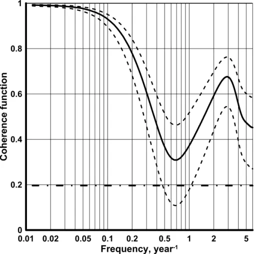
The values of the coherence function between SSN and TSI, which has been ob-tained from the spectral matrix corresponding to Eqs. (12) and (13), are very high (above 0.9) at frequencies below 0.14 year−1 (Fig. 4). This means that the linear de-pendence between TSI and SSN at those frequencies is responsible for at least 80 % of time series’ variances. At frequencies above 0.28 year−1, the coherence stays below

15

0.7 but this weaker dependence is less important as the spectral density values there are much smaller than at the low-frequency band (Fig. 2).

4.2 Reconstruction

A seemingly obvious way to obtain past monthly values of TSI back to January 1749 would be to simulate TSI in accordance with Eq. (12), starting from December 1978 and

20

substituting the observed SSN values at each step into the past. To start this recursive process, one will also need three (in accordance with the order p of the AR model) first monthly values of TSI and SSN in 1979. However, this approach to reconstruction would be wrong because it depicts values of TSI as a function offuturevalues of both TSI and SSN:

25

x1,n=ϕ

(1)

11x1,n+1+ϕ (1)

12x2,n+1+. . .+ϕ (3)

11x1,n+3+ϕ (3)

(15)

CPD

11, 4701–4728, 2015

climatology

Title Page

Tables Figures

◭ ◮

Back Close

Full Screen / Esc

Discussion

P

a

per

|

Discussion

P

a

per

|

Discussion

P

a

per

|

Discussion

P

a

per

|

Though the SSN datax2,n is known, the dependence ofx1,n upon its unknown future

values makes the linear operator Eq. (14) physically unrealizable. If, nevertheless, past values of TSI are simulated in accordance with Eq. (14), its properties in the frequency domain will be the same as before but the AR coefficients would be different from those in Eq. (12).

5

Therefore, the past values of TSI should be reconstructed starting from the earliest observation date of SSN, that is, from January 1749. It means using the first of the Eq. (12) to reconstruct the past values ofx1,n on the basis of its past values and the

known past values ofx2,n:

x1,n≈0.32x1,n−1+0.31x2,n−1+0.11x1,n−2+0.02x2,n−2+0.07x1,n−3−0.07x2,n−3, (15)

10

wheren=1,. . .,N1. The first three values of TSI for 1749 will not include the depen-dence of TSI upon its past values. The unknown past values of the innovation sequence

a1,nare not included into the reconstructed TSI time series shown in Fig. 5.

The differences between the estimates of the mean values and between the variance estimates for the observed (1979–2014, N2−N1=432) and reconstructed

15

(April 1749–December 1978,N1−3=2757) TSI time series lie within respective con-fidence intervals for the estimates at a concon-fidence level 0.90. The concon-fidence inter-vals were calculated with account for the behavior of respective correlation functions (see Yaglom, 1986). The SSN variance estimates for 1749–1978 and 1979–2014 were 4468 number2 and 5471 number2, respectively. This drop in the SSN variance

20

in the past and the lack of the innovation sequence a1,n in Eq. (15) explain the

de-crease in the TSI variance from 0.170 (W m−2)2for the observed data in 1979–2014 to 0.107 (W m−2)2 for the restored time series in 1749–1978. The probability distribution functions of the observed and restored time series significantly differ from the Gaus-sian, which should have been expected due to the presence of the 11 year cycle.

25

As seen from Fig. 6, the agreement between the spectra of observed (1979–2014) and restored TSI data (1749–1978) is quite satisfactory. Note that though the cross-correlation coe_fficient between SSN and the reconstructed TSI is less than 1, the

(16)

CPD

11, 4701–4728, 2015

climatology

Title Page

Tables Figures

◭ ◮

Back Close

Full Screen / Esc

Discussion

P

a

per

|

Discussion

P

a

per

|

Discussion

P

a

per

|

Discussion

P

a

per

|

herence between them (not shown) equals 1 at all frequencies because, according to Eq. (15), TSI is a linear function of SSN. The spectrum of the time series restored through the regression Eq. (11) stays below the spectrum of the TSI time series re-constructed through Eq. (15) at all frequencies up to 0.5 year−1, which illustrates the relative incapability of the correlation/regression approach.

5

To further estimate these differences in reconstructions, consider the results obtained for the interval from 1979 through 2014 over which the values of TSI are known from observations. First, according to Eq. (11), the variance of the TSI time series recon-structed through linear regression isϕ2σ₂2≈0.101(W m−2)2 while the variance of the observed TSI time series is 0.170(W m−2)2. The variance of the TSI time series

re-10

stored through Eq. (15) is 0.131(W m−2)2. In other words, the AR approach allows one to reconstruct a substantially larger share of the process (actually, by about 22 %). If the reconstruction error is defined as the difference between the observed and re-constructed time series of TSI, the variance of the error time series will be 0.069 and 0.058(W m−2)2 for the time series reconstructed on the basis of Eqs. (11) and (15),

15

respectively.

Comparing the spectral density of the observed TSI with those of the two recon-structed time series (shown in Fig. 7 for the lower frequency band where the spectral energy is high), one can see that

– the TSI spectrum obtained through regression is mostly negatively biased with

20

respect to the spectrum of TSI obtained through Eq. (15) and

– this spectrum (which, according to Eq. (11), is identical to the SSN spectrum up to a multiplier) differs from the spectrum of the observed TSI.

In this case, the discrepancy between the two spectra is not large because of the dominance of the 11 year solar cycle which is reproduced with both methods. But the

25

(17)

CPD

11, 4701–4728, 2015

climatology

Title Page

Tables Figures

◭ ◮

Back Close

Full Screen / Esc

Discussion

P

a

per

|

Discussion

P

a

per

|

Discussion

P

a

per

|

Discussion

P

a

per

|

A more spectacular results would be obtained if one were to restore the contribution of El Niño – Southern Oscillation (ENSO) to, say, the global surface temperature (GST), or the Atlantic Multidecadal Oscillation (AMO). In those cases, the correlation coeffi -cient between GST and ENSO or between AMO and ENSO would be very close to zero (−0.06 between AMO and the sea surface temperature in the ENSO area 3.4) while

5

the coherence function estimates will significantly differ from zero in the frequency band between approximately 0.15 and 0.40 year−1. In this latter case, the linear-regression contribution of ENSO to GST will be less than 0.4 % while the proper autoregressive approach will show a contribution of 25 to more than 50 % of spectral energy within the respective frequency band (see Privalsky, 2015). In the case of GST and ENSO,

10

the linear regression contribution is less than 10 % while the autoregressive approach gives from 25 to 66 % between approximately 0.1 and 0.4 year−1.

5 Conclusions

The main goal of this study was to show that the task of reconstructing past values of a bi-variate time series on the basis of simultaneous observations of its components

15

during a relatively short time interval should be treated within the framework of time series analysis. This is done in the following manner:

a. build and analyze an autoregressive model of the bivaraite time series in the time and frequency domains,

b. use the model to simulate the missing time series component into the past starting

20

from the earliest observation of the proxy data and substituting the known proxy data at each step into the difference equation for the unknown time series,

c. verify that basic statistical properties of the reconstructed component do not differ much from the properties known from observations.

(18)

CPD

11, 4701–4728, 2015

climatology

Title Page

Tables Figures

◭ ◮

Back Close

Full Screen / Esc

Discussion

P

a

per

|

Discussion

P

a

per

|

Discussion

P

a

per

|

Discussion

P

a

per

|

Note that the method does not require any filtering of the time series, be it a prewhiten-ing or any other type of linear filters.

This approach based upon time series analysis and upon previous research in pale-oclimatology was applied here to the time series containing monthly values of the total solar irradiance of the Earth (TSI) measured during the interval from 1979 through 2014

5

and the sunspot numbers observed from 1749 through 2014 to produce an estimate of monthly TSI values from 1749 through 1978.

On the whole, it can be said that the statistical properties of the reconstructed TSI data such as its variance and spectral density do not disagree with respective proper-ties of the observed TSI and that the time series approach produced better results than

10

the regression-based reconstruction.

This approach to reconstruction is recommended for all cases when the spectra of the time series components differ from a constant (white noise) and/or from each other and when the cross-correlation function between the components contains more than just one statistically significant value.

15

It must be also stressed that the autoregressive model introduced here emerges as a natural extension of the linear regression equation for the case of multivariate random functions. In particular, it means that the use of the moving average (MA) or mixed autoregressive – moving average (ARMA) models would be illogical in such cases.

Acknowledgements. The authors are grateful to F. Clette for providing the sunspot time

se-20

ries and commenting on it and to J. Guiot for his important comments and suggestions. A. Gluhovsky acknowledges support from the National Science Foundation under Grant no. AGS-1 050 588.

References

Bendat, J. and Piersol, A.: Measurement and Analysis of Random Data, Wiley, New York, 1966.

25

(19)

CPD

11, 4701–4728, 2015

climatology

Title Page

Tables Figures

◭ ◮

Back Close

Full Screen / Esc

Discussion

P

a

per

|

Discussion

P

a

per

|

Discussion

P

a

per

|

Discussion

P

a

per

|

Box, G. and Jenkins, J.: Time Series Analysis, Forecasting and Control, Holden-Day, San Fran-cisco, 1970.

Box, G. E. P., Jenkins, G. M., Reinsel, G. C., and Ljung, G. M.: Time Series Analysis: Forecast-ing and Control, 5th Edn., Wiley, London, 2015.

Bradley, R. S.: Paleoclimatology: Reconstructing Climates of the Quaternary, 3rd Edn., Elsevier,

5

Boston, 2015.

Choi, B. and Cover, T.: An information-theoretic proof of Burg’s maximum entropy spectrum, P. IEEE, 72, 1094–1096, 1984.

Clette, F., Svalgaard, L., Vaquero, J., and Cliver, E.: Revisiting the sunspot number, a 400-year perspective on the solar cycle, Space Sci. Rev., 186, 35–103, 2014.

10

Davis, B. A. S., Brewer, S., Stevenson, A. C., Guiot, J., and Data Contributors: The temperature of Europe during the Holocene reconstructed from pollen data, Quaternary Sci. Rev., 22, 1701–1716, 2003.

Douglass, A. E.: Weather cycles in the growth of big trees, Mon. Weather Rev., 37, 225–237, 1909.

15

Douglass, A. E.: A method of estimating rainfall by the growth of trees, in: The Climatic Factor, edited by: Huntington, E., Carnegie Inst. Wash. Publ., Washington, 101–122, 1914.

Douglass, A. E.: Climatic Cycles and Tree-Growth: a Study of the Annual Rings of Trees in Relation to Climate and Solar Activity, Carnegie Inst. Wash. Publ., 289, Vol. 1, Washington, 1–127, 1919.

20

Douglass, A. E.: Climatic Cycles and Tree-Growth: a Study of the Annual Rings of Trees in Relation to Climate and Solar Activity, Carnegie Inst. Wash. Publ., 289, Vol. 2, Washington, 1–166, 1928.

Douglass, A. E.: Climatic Cycles and Tree-Growth: a Study of Cycles, Carnegie Inst. Wash. Publ., 289, Vol. 3, Washington, 1–171, 1936.

25

Emery, W. and Thomson, R.: Data Analysis Methods in Physical Oceanography, 2nd Edn., Elsevier, Amsterdam, 2004.

Fritts, H. C.: Tree Rings and Climate, Academic Press, London, 1976.

Fröhlich, C.: Observations of irradiance variations, Space Sci. Rev., 94, 15–24, 2000.

Fröhlich, C.: Evidence of a long-term trend in total solar irradiance, Astron. Astrophys., 501,

30

L27–L30, doi:10.1051/0004-6361/200912318, 2009.

(20)

CPD

11, 4701–4728, 2015

climatology

Title Page

Tables Figures

◭ ◮

Back Close

Full Screen / Esc

Discussion

P

a

per

|

Discussion

P

a

per

|

Discussion

P

a

per

|

Discussion

P

a

per

|

Gelfand, I. and Yaglom, A.: Calculation of the amount of information about a random func-tion contained in another such funcfunc-tion, Uspekhi Matematicheskikh Nauk, 12, 3–52, 1957, English translation: American Mathematical Society Translation Series, 2, 199–246, 1959. Granger, C. W. J.: Investigating causal relations by econometric models and crossspectral

methods, Econometrica, 37, 424–438, 1969.

5

Granger, C. W. J. and Hatanaka, M.: Spectral Analysis of Economic Time Series, Princeton University Press, Princeton, New Jersey, 1964.

Guiot, J.: The extrapolation of recent climatological series with spectral canonical regression, J. Climatol., 5, 325–335, 1985.

Guiot, J.: ARMA techniques for modelling tree-ring response to climate and for reconstructing

10

variations of paleoclimates, Ecol. Model., 33, 149–171, 1986.

Guiot, J., Berger, A., Munaut, A. V., and Till, C.: Some new mathematical procedures in den-droclimatology, with examples from Switzerland and Morocco, Tree-Ring Bull., 42, 33–48, 1982.

Hannan, E. and Quinn, B.: The determination of the order of an autoregression, J. R. Stat. Soc.,

15

41, 190–195, 1979.

Haslett, J., Whiley, M., Bhattacharya, S., Salter-Townshend, M., Wilson, S. P., Allen, J. R. M., Huntley, B., and Mitchell, F. J. G.: Bayesian palaeoclimate reconstruction, J. R. Stat. Soc., 169, 395–438, 2006.

Kolmogorov, A. N.: On the problem of the suitability of forecasting formulas found by statistical

20

methods, Journal of Geophysics, 3, 78–82, 1933 (in Russian), English translation in Selected Works by A. N. Kolmogorov, Vol. II. Probability Theory and Mathematical Statistics, Springer, Dordrecht, 169–175, 1992.

Maxwell, J. T., Harley, G. L., and Matheus, T. J.: Dendroclimatic reconstructions from multiple co-occurring species: a case study from an old-growth deciduous forest in Indiana, USA,

25

Int. J. Climatol., 35, 860–870, 2015.

Parzen, E.: Multiple time series: determining the order of autoregressive approximating schemes, in: Multivariate Analysis – IV, North Holland Publishing Company, Amsterdam, 283–295, 1977.

Privalsky, V.: On studying relations between time series in climatology, Earth Syst. Dynam., 6,

30

389–397, doi:10.5194/esd-6-389-2015, 2015.

(21)

CPD

11, 4701–4728, 2015

climatology

Title Page

Tables Figures

◭ ◮

Back Close

Full Screen / Esc

Discussion

P

a

per

|

Discussion

P

a

per

|

Discussion

P

a

per

|

Discussion

P

a

per

|

Bernoulli Society on Mathematical Stat. Theory and Applications, 8–14 September, 1986, Tashkent, Vol. 2, VNU Science Press, Utrecht, 651–654, 1987.

Robinson, E.: Multichannel Time Series Analysis with Digital Computer Programs, Holden-Day, San Francisco, 1967.

Robinson, E. and Treitel, S.: Geophysical Signal Analysis, Prentice-Hall, Englewood Cliffs, NJ,

5

1980.

Santos, J. A., Carneiro, M. F., Correia, A., Alcoforado, M. J., Zorita, E., and Gómez-Navarro, J. J.: New insights into the reconstructed temperature in Portugal over the last 400 years, Clim. Past, 11, 825–834, doi:10.5194/cp-11-825-2015, 2015.

Steinhilber, F., Beer, J., and Fröhlich, C.: Total solar irradiance during the Holocene, Geophys.

10

Res. Lett., 36, L19704, doi:10.1029/2009GL040142, 2009.

Tingley, M. P. and Huybers, P.: A Bayesian algorithm for reconstructing climate anomalies in space and time, Part I: development and applications to paleoclimate reconstruction prob-lems, J. Climate, 23, 2759–2781, 2010.

Tingley, M. P., Craigmile, P. F., Haran, M., Li, B., Mannshardt, E., and Bala Rajaratnam, B.:

15

Piecing together the past: statistical insights into paleoclimatic reconstructions, Quaternary Sci. Rev., 35, 1–22, 2012.

Visser, H. and Molenaar, J.: Kalman filter analysis in dendroclimatology, Biometrics, 44, 929– 940, 1988.

von Storch, H., Zorita, E., Jones, J. M., Dimitriev, Y., Gonzalez-Rouco, F., and Tett, S. F. B:

20

Reconstructing past climate from noisy data, Science, 306, 679–682, 2004.

Yaglom, A. M.: Correlation Theory of Stationary and Related Functions, Springer, New York, 1986.

(22)

CPD

11, 4701–4728, 2015

climatology

Title Page

Tables Figures

◭ ◮

Back Close

Full Screen / Esc

Discussion

P

a

per

|

Discussion

P

a

per

|

Discussion

P

a

per

|

Discussion

P

a

per

|

(23)

CPD

11, 4701–4728, 2015

climatology

Title Page

Tables Figures

◭ ◮

Back Close

Full Screen / Esc

Discussion

P

a

per

|

Discussion

P

a

per

|

Discussion

P

a

per

|

Discussion

P

a

per

|

Figure 2.Autoregressive spectral estimates of monthly TSI (black) and SSN (blue) with ap-proximate 90 % confidence bands (dashed lines), 1979–2014.

(24)

CPD

11, 4701–4728, 2015

climatology

Title Page

Tables Figures

◭ ◮

Back Close

Full Screen / Esc

Discussion

P

a

per

|

Discussion

P

a

per

|

Discussion

P

a

per

|

Discussion

P

a

per

|

(25)

CPD

11, 4701–4728, 2015

climatology

Title Page

Tables Figures

◭ ◮

Back Close

Full Screen / Esc

Discussion

P

a

per

|

Discussion

P

a

per

|

Discussion

P

a

per

|

Discussion

P

a

per

|

Figure 4.Estimated coherence function TSI-SSN, 1979–2014, with approximate 90 % confi-dence band (dashed lines, see Privalsky et al., 1987, 2015). The horizontal line is the approxi-mate 90 % upper limit for the true zero coherence estiapproxi-mate.

(26)

CPD

11, 4701–4728, 2015

climatology

Title Page

Tables Figures

◭ ◮

Back Close

Full Screen / Esc

Discussion

P

a

per

|

Discussion

P

a

per

|

Discussion

P

a

per

|

Discussion

P

a

per

|

(27)

CPD

11, 4701–4728, 2015

climatology

Title Page

Tables Figures

◭ ◮

Back Close

Full Screen / Esc

Discussion

P

a

per

|

Discussion

P

a

per

|

Discussion

P

a

per

|

Discussion

P

a

per

|

Figure 6.AR spectra of monthly observed and reconstructed TSI data for 1749–1978 (black and blue lines, respectively) with approximate 90 % confidence bands (dashed lines). The spec-trum of TSI reconstructed through the regression Eq. (12) is shown with the green line.

(28)

CPD

11, 4701–4728, 2015

climatology

Title Page

Tables Figures

◭ ◮

Back Close

Full Screen / Esc

Discussion

P

a

per

|

Discussion

P

a

per

|

Discussion

P

a

per

|

Discussion

P

a

per

|