Off-line algorithm for calculation of vertical tracer transport in the troposphere due to deep convection

(1)

ACPD

12, 20239–20289, 2012

O_ff-line algorithm for calculation of vertical

tracer transport

D. A. Belikov et al.

Title Page

Abstract Introduction

Conclusions References

Tables Figures

◭ ◮

Back Close

Full Screen / Esc

Printer-friendly Version

Interactive Discussion

Discussion

P

a

per

|

Dis

cussion

P

a

per

|

Discussion

P

a

per

|

Discussio

n

P

a

per

Atmos. Chem. Phys. Discuss., 12, 20239–20289, 2012 www.atmos-chem-phys-discuss.net/12/20239/2012/ doi:10.5194/acpd-12-20239-2012

Atmospheric Chemistry and Physics Discussions

This discussion paper is/has been under review for the journal Atmospheric Chemistry and Physics (ACP). Please refer to the corresponding final paper in ACP if available.

O

_ff

-line algorithm for calculation of

vertical tracer transport in the

troposphere due to deep convection

D. A. Belikov1, S. Maksyutov1, M. Krol2,3,4, A. Fraser5, M. Rigby6, H. Bian7, A. Agusti-Panareda8, D. Bergmann9, P. Bousquet10, P. Cameron-Smith9,

M. P. Chipperfield11, A. Fortems-Cheiney10, E. Gloor11, K. Haynes12,13, P. Hess14, S. Houweling2,3, S. R. Kawa7, R. M. Law13, Z. Loh13, L. Meng15, P. I. Palmer5, P. K. Patra16, R. G. Prinn17, R. Saito16, and C. Wilson11

1

Center for Global Environmental Research, National Institute for Environmental Studies, 16-2 Onogawa, Tsukuba, Ibaraki, 305-8506, Japan

2

SRON Netherlands Institute for Space Research, Sorbonnelaan 2, 3584 CA Utrecht, The Netherlands

3

Institute for Marine and Atmospheric Research Utrecht (IMAU), Princetonplein 5, 3584 CC Utrecht, The Netherlands

4

Wageningen University and Research Centre, Droevendaalsesteeg 4, 6708 PB Wageningen, The Netherlands

5

School of GeoSciences, University of Edinburgh, King’s Buildings, West Mains Road, Edinburgh, EH9 3JN, UK

6

(2)

ACPD

12, 20239–20289, 2012

Title Page

Tables Figures

◭ ◮

Back Close

Full Screen / Esc

Discussion

P

a

per

|

Dis

cussion

P

a

per

|

Discussion

P

a

per

|

Discussio

n

P

a

per

|

7

Goddard Earth Sciences and Technology Center, NASA Goddard Space Flight Center, Code 613.3, Greenbelt, MD 20771, USA

8

ECMWF, Shinfield Park, Reading, Berks, RG2 9AX, UK

9

Atmospheric, Earth, and Energy Division, Lawrence Livermore National Laboratory, 7000 East Avenue, Livermore, CA 94550, USA

10

Universite de Versailles Saint Quentin en Yvelines (UVSQ), Gif-sur-Yvette, France

11

Institute for Climate and Atmospheric Science, School of Earth and Environment, University of Leeds, Leeds, LS2 9JT, UK

12

Department of Atmospheric Science, Colorado State University, Fort Collins, CO 80523, USA

13

Centre for Australian Weather and Climate Research, CSIRO Marine and Atmospheric Research, 107-121 Station St., Aspendale, VIC 3195, Australia

14

Cornell University, 2140 Snee Hall, Ithaca, NY 14853, USA

15

Department of Geography and Environmental Studies Program, Western Michigan University, Kalamazoo, MI 49008, USA

16

Research Institute for Global Change/JAMSTEC, 3173-25 Show-machi, Yokohama, 2360001, Japan

17

Center for Global Change Science, Building 54, Massachusetts Institute of Technology, Cambridge, MA 02139, USA

Received: 25 May 2012 – Accepted: 17 July 2012 – Published: 14 August 2012

Correspondence to: D. A. Belikov (dmitry.belikov@nies.go.jp)

(3)

ACPD

12, 20239–20289, 2012

Title Page

Tables Figures

◭ ◮

Back Close

Full Screen / Esc

Discussion

P

a

per

|

Dis

cussion

P

a

per

|

Discussion

P

a

per

|

Discussio

n

P

a

per

Abstract

A modified cumulus convection parametrisation scheme is presented. This scheme computes the mass of air transported upward in a cumulus cell using conservation of moisture and a detailed distribution of convective precipitation provided by a reanalysis dataset. The representation of vertical transport within the scheme includes

entrain-5

ment and detrainment processes in convective updrafts and downdrafts. Output from the proposed parametrisation scheme is employed in the National Institute for Envi-ronmental Studies (NIES) global chemical transport model driven by JRA-25/JCDAS reanalysis. The simulated convective precipitation rate and mass fluxes are compared

with observations and reanalysis data. A simulation of the short-lived tracer222Rn is

10

used to further evaluate the performance of the cumulus convection scheme. Simulated

distributions of222Rn are validated against observations at the surface and in the free

troposphere, and compared with output from models that participated in the

TransCom-CH₄Transport Model Intercomparison. From this comparison, we demonstrate that the

proposed convective scheme can successfully reproduce deep cloud convection.

15

1 Introduction

Deep cumulus convection (DCC) plays an important role in the hydrological cycle of the climate system, the dynamics of the atmospheric circulation and the transport of trace gases within the troposphere. Indeed, the major sources of uncertainty in climate models are associated with the representation of cumulus convection. DCC also

af-20

fects atmospheric chemistry indirectly through latent heating and contributions to the budgets of solar and infrared radiation (Lawrence and Salzmann, 2008).

Deep convective updrafts extend from the surface to the upper troposphere, with typ-ical verttyp-ical velocities of several meters per second. These rapid updrafts are accom-panied by rapid downdrafts, which together result in considerable vertical mixing and

25

(4)

ACPD

12, 20239–20289, 2012

Title Page

Tables Figures

◭ ◮

Back Close

Full Screen / Esc

Discussion

P

a

per

|

Dis

cussion

P

a

per

|

Discussion

P

a

per

|

Discussio

n

P

a

per

|

Crutzen, 1990). Air masses associated with DCC can reach altitudes above the zero radiative heating level in the tropical tropopause layer, allowing detrained air to slowly ascend into the lower stratosphere (Folkins et al., 1999; Fueglistaler et al., 2004). The rapid updrafts associated with DCC occasionally even cause direct penetration of tro-pospheric air into the lower stratosphere, which can last up to several hours. After rapid

5

ascent from the surface layer in DCC, tracers can be advected over long distances by the strong zonal winds that prevail in the upper atmosphere (Allen et al., 1996; Zau-cker et al., 1996). This relationship illustrates the important role that convection plays

in long-range tracer transport. Along with large-scale advection and vertical diffusion,

cumulus convection is one of the most important transport processes affecting

atmo-10

spheric tracers.

General circulation models (GCMs) and chemical transport models (CTMs) are un-able to explicitly resolve convection due to its small spatial scale relative to synoptic-scale processes and the resolution of model grids. Cumulus convection must there-fore be parametrised in global models. This has motivated the development of a large

15

number of different parametrisations of cumulus convection. Of these parametrisations,

those based on plume ensemble formulations and those based on bulk formulations are the most widely used in tracer transport applications (Arakawa, 2004; Lawrence and Rasch, 2005). Regardless of the approach used in a cumulus convection parametrisa-tion, a set of equations must be solved. On-line coupling of a CTM with a GCM can

20

offer significant advantages if both models are running simultaneously. This approach

allows tracer transport to be calculated within the CTM while the GCM provides the meteorological variables (including parametrised fields) that are used to drive tracer transport.

The options available for on-line CTMs are generally not available for off-line

mod-25

(5)

ACPD

12, 20239–20289, 2012

Title Page

Tables Figures

◭ ◮

Back Close

Full Screen / Esc

Discussion

P

a

per

|

Dis

cussion

P

a

per

|

Discussion

P

a

per

|

Discussio

n

P

a

per

parametrisation schemes in off-line CTMs presents a significant challenge (Mahowald

et al., 1995, 1997).

Previous studies have demonstrated that transport model simulations of the

distri-bution of222Rn fields are strongly sensitive to the parametrisation used to represent

cumulus convection (Brost and Chatfield, 1989; Jacob et al., 1997). 222Rn is almost

5

completely insoluble in water, so that it is removed from the atmosphere solely by ra-dioactive decay. The sensitivity to the parametrisation schemes and the relatively

sim-ple life cycle make222Rn an excellent tracer for evaluating the performance of transport

models in simulations of short-range transport over continental and remote oceanic re-gions (Allen et al., 1996; Dentener et al., 1999).

10

Although222Rn has long been recognized as a useful tracer for evaluating the

per-formance of transport models, it has several disadvantages related to source uncer-tainties. The most frequently used fluxes (Jacob et al., 1997) are accurate to within 25 % globally and to within a factor of two regionally. The main factors controlling

spa-tial variations in222Rn flux are depth of aerated soil, soil 226Ra concentrations (222Rn

15

precursor) and emanation rate. The main factors determining temporal variations are precipitation and soil moisture. Shallow water tables and frost cover can be a cause of temporal but also of spatial variation (Conen, 2004).

Previous studies have performed detailed examinations of the influence of

convec-tive mixing on222Rn and other short-lived tracers’ distributions in the troposphere

(Ma-20

howald et al., 1995, 1997; Allen et al., 1996; Li and Chang, 1996; Jacob et al., 1997; Rasch et al., 1997; Olivi ´e et al., 2004; Zhang at el., 2008). Although measurements of atmospheric radon concentration by distributed observatories provide good reference points for model evaluation, there remains a lack of suitable measurements of radon concentration in the free troposphere (Zhang et al., 2008). Recent studies (e.g. Tost

25

et al., 2010) have focused on evaluating how the formulations of convective schemes influence simulated tracer distributions and quantifying uncertainties in trace gases

(H2O,

222

Rn, CO, HCHO, HNO3 and O3) due to the parametrisation of convection.

(6)

ACPD

12, 20239–20289, 2012

Title Page

Tables Figures

◭ ◮

Back Close

Full Screen / Esc

Discussion

P

a

per

|

Dis

cussion

P

a

per

|

Discussion

P

a

per

|

Discussio

n

P

a

per

|

tracer transport in a global off-line 3-D chemical transport model and to diagnose the

updraft mass flux, convective precipitation and cloud top height performing various

model simulations using different meteorological (re)analyses (Feng et al., 2011).

Uncertainties in convective transport processes may also be quantified by compar-ing the output of a variety of models that employ a range of cumulus parametrisations.

5

Although the primary focus of the TransCom-CH4 Transport Model Intercomparison

(TMI) was CH4, the contributing models also simulated the distributions of several

auxiliary tracers, including 222Rn (Patra et al., 2011). The TransCom-CH₄ TMI

simu-lation of 222Rn is similar to the simulation protocol specified by Jacob et al. (1997)

The surface flux of 222Rn is set to 1.66×10−20mol m−2s−1 for land areas between

10

60◦S and 60◦N, to 8.3×10−23mol m−2s−1 for oceans between 60◦S and 60◦N and

to 8.3×10−23mol m−2s−1 for arctic regions (60◦–70◦N). This surface flux distribution

ensures consistency with radon simulations conducted in conjunction with the World Climate Research Programme (WCRP) and other previous studies (e.g. Mahowald et al., 1997; Zhang et al., 2008).

15

This work describes an adaptation of the cumulus convection parametrisation scheme used in the National Institute for Environmental Studies (NIES) transport model. This adaptation aims to improve model performance by achieving more realistic simulations of vertical mixing and tracer transport. The paper is organized as follows. The DCC parametrisation and model formulation are described in Sect. 2. The

reanal-20

ysis convective precipitation rates and simulated convective mass fluxes are validated against reanalysis and observational data in Sect. 3. The simulated surface

concentra-tions and vertical profiles of222Rn are evaluated relative to in situ observations from

aircraft and surface stations and compared with output from models that contributed

to the TransCom-CH4TMI in Sect. 4. Here we also analyzed performance of the other

25

TransCom-CH4 transport models. The results and conclusions of the study are

(7)

ACPD

12, 20239–20289, 2012

Title Page

Tables Figures

◭ ◮

Back Close

Full Screen / Esc

Discussion

P

a

per

|

Dis

cussion

P

a

per

|

Discussion

P

a

per

|

Discussio

n

P

a

per

2 Model formulation

2.1 Off-line calculation of convective mass flux

In this work, the method for calculating cumulus convective vertical mass fluxes from precipitation rates is modified from that developed by Austin and Houze (1973) and first implemented by Feichter and Crutzen (1990). The method is built on the basic

5

assumption that the mass of air transported upward in a cumulus cell is related to the amount of precipitation that the cell produces. This premise is based on empirical data and simplified dynamic cell model. The upward mass transport can therefore be computed from conservation of water if the amount of precipitation generated by the

cell is known. Following Austin and Houze (1973), the mass of airMU rising through

10

the level of maximum upward fluxζis given by

MU(ζ)=C/

z_top

Z

z_base f(z)

EU(qE−qU)−

dqU

dz

dz. (1)

The parameters of Eq. (1) are defined as follows:

C– total amount of water condensed in the convective cloud cell (kg),

f(z) – shape function,

15

EU– updraft entrainment rate (km

−1 ),

qE– mixing ratio of water in the environment,

qU– mixing ratio of water in the updraft,

z– vertical level (m),

zbase,ztop– altitudes of the base and top levels of the cloud cell (m).

20

The mass of air rising vertically through any levelzis then parametrised as

(8)

ACPD

12, 20239–20289, 2012

Title Page

Tables Figures

◭ ◮

Back Close

Full Screen / Esc

Discussion

P

a

per

|

Dis

cussion

P

a

per

|

Discussion

P

a

per

|

Discussio

n

P

a

per

|

where the level of maximum upward fluxζ is approximated from observations

accord-ing to the expression

ζ=zbase+α ztop−zbase

. (3)

The parameterα is set equal 0.75 in the tropics and 0.5 in midlatitudes (Austin and

Houze, 1973). Following Feichter and Crutzen (1990), the shape functionf(z) is defined

5

as

f(z)=

( ₁

2−E_U

2 exp (EU(z−ζ))−EUexp (2 (z−ζ))

,zbase< z < ζ

1− z−ζ /ztop−ζ

2

, ζ≤z < ztop

(4)

The entrainment rate is assumed to remain constant with altitude (Austin and Houze, 1973), and is defined as

EU=

a

0.13 ztop−zbase−1

(km

−1_), _a

=0.2. (5)

10

The total amount of water condensed in the cloud during the life-cycle of the convective cell is given by

C=x1×Pc, (6)

wherePc denotes the total amount of convective precipitation at the surface (kg) and

x₁is a constant in the range 2. . .10 with a typical value between 3 and 4 (Austin and

15

Houze, 1973).

In tracer transport applications, the vertical convective mass flux MFU is of primary

practical importance. This flux can be determined as MFU=MU/(S×∆t), where S is

the area of the model grid cell, and_∆t is the time step used in the model integration.

The total amount of convective precipitation can be similarly determined asPc=PR×

(9)

ACPD

12, 20239–20289, 2012

Title Page

Tables Figures

◭ ◮

Back Close

Full Screen / Esc

Discussion

P

a

per

|

Dis

cussion

P

a

per

|

Discussion

P

a

per

|

Discussio

n

P

a

per

S×_∆t, whereP_R is the surface convective precipitation rate (kg m−2s−1) provided by

a reanalysis dataset. The equation for the vertical convective mass flux MFUis then

MFU(ζ)=x1·PR/

z_top

Z

zbase f(z)

EU(qE−qU)−

dqU

dz

dz. (7)

By contrast, the updraft mass flux MFUin the original Kuo-type scheme (Tiedtke, 1989)

is determined as the ratio of low-level moisture convergence (ML) to the mixing ratio of

5

water vapour at cloud base (qbase):

MF_U=ML/qbase (8)

M_Lis obtained by integrating the total horizontal moisture convergence below the cloud

base:

ML=−

 

1

Z

σ_C

∇_σ(pS·V ·q)d σ−Mc



+Sevap (9)

10

whereV is the horizontal wind velocity vector with longitudinal and latitudinal

compo-nents (uv);σ=p/ps, wherepandps are the atmospheric and the surface pressures;

σcis the cloud base level,Mcis the air mass below cloud base level andSevapis the

sur-face evaporation. This off-line algorithm based on moisture balance introduces more

errors in estimates of cloud updraft and precipitation than the more straightforward

15

approach of Eq. (7) because it involves additional spatial and temporal interpolations between the reanalysis model grid, the reanalysis data grid and the transport model

grid. It may be a reason for underprediction of222Rn in the upper atmosphere in the

previous version of NIES TM (Maksyutov et al., 2008).

The detrainment rate of mass from convective plumes due to turbulent mass

ex-20

(10)

ACPD

12, 20239–20289, 2012

Title Page

Tables Figures

◭ ◮

Back Close

Full Screen / Esc

Discussion

P

a

per

|

Dis

cussion

P

a

per

|

Discussion

P

a

per

|

Discussio

n

P

a

per

|

Tiedtke, 1989):

DU=δU×MFU. (10)

The entrainment and detrainment rate coefficients are the same as those employed by

Tiedtke (1989):εU=δU=1×10

−4

(m−1).

Following Johnson (1976), the downdraft mass flux is defined to be directly

propor-5

tional to the upward mass flux:

MFt_D₌γMFb_U, (11)

where MFt_D is the downdraft mass flux at cloud top, MFb_U is the updraft mass flux at

cloud base and γ is a parameter equal to−0.2 (Tiedtke, 1989). The parametrisation

used for entrainment and detrainment in downdrafts is identical to that used in updrafts,

10

with entrainment and detrainment rate coefficientsεD=δD=2×10

−4

(m−1) (Tiedtke,

1989).

Following the determination of the updraft and downdraft mass fluxes, tracer trans-port by cumulus convection is simulated using the explicit scheme presented by Maksyutov et al. (2008). The tracer concentration is estimated at each level of the

15

convective column sequentially from bottom to top using known updraft, downdraft,

en-trainment and deen-trainment mass fluxes along with differences in tracer concentration

differences between the convective column and the ambient environment. The tracer

tendency in the surrounding environmental air is then calculated according to the same tracer fluxes.

20

The implementation of this convective parametrisation scheme requires a priori knowledge of convective precipitation rate at the surface and the levels of cloud top and cloud base. These parameters must be supplied by a meteorological reanalysis dataset or calculated using the Kuo parametrisation scheme (Kuo, 1965, 1974). This latter technique has been implemented in the National Center for Atmospheric

Re-25

(11)

ACPD

12, 20239–20289, 2012

Title Page

Tables Figures

◭ ◮

Back Close

Full Screen / Esc

Discussion

P

a

per

|

Dis

cussion

P

a

per

|

Discussion

P

a

per

|

Discussio

n

P

a

per

et al. (1994). The level of the cloud base (σb) is defined as the lowest level where

con-densation would occur during dry adiabatic ascent, which is often referred to as the lifting condensation level. This level is identified by slightly perturbing the humidity and temperature fields at levels below 700 hPa and determining where condensation would occur if the perturbed air parcel were lifted adiabatically. The level of the cloud top is

5

identified based on the assumptions that enthalpy is greater inside clouds than out-side clouds and that enthalpy decreases upward due to entrainment and detrainment. At the level of cloud top, the total thermodynamic energy inside the cloud should equal the total thermodynamic energy outside; accordingly, cloud top is defined as the level of zero buoyancy, with a minor overshoot of 3 K that accounts for the upward momentum

10

of the convective updraft (Kuo, 1974). The upper boundary of the cloud is confined to

altitudes below the 150 hPa isobaric level. Clouds with thicknesses less than∆σ=0.1

are excluded from consideration.

2.2 The NIES global tracer transport model

The cumulus parametrisation scheme, in which the vertical convective mass flux

cal-15

culated using Eq. (7) is incorporated into the National Institute for Environmental

Stud-ies off-line global Transport Model (NIES TM). The goal of this parametrisation is to

improve the accuracy of NIES TM simulations of vertical tracer transport in the tropo-sphere by improving the representation of tracer transport in DCC.

The NIES TM is designed to simulate natural and anthropogenic synoptic-scale

vari-20

ations in atmospheric constituents at diurnal, seasonal and interannual timescales. The model uses a mass-conservative flux-form formulation that consists of a third-order van Leer advection scheme and a horizontal dry-air mass flux correction (Heimann and Keeling, 1989). The horizontal latitude–longitude grid is a reduced rectangular grid (i.e. the grid size is doubled several times approaching the poles; Kurihara, 1965), with an

25

initial spatial resolution of 2.5◦×2.5◦(Belikov et al., 2011).

The parametrisation of turbulent diffusivity follows the approach used by Hack

(12)

ACPD

12, 20239–20289, 2012

Title Page

Tables Figures

◭ ◮

Back Close

Full Screen / Esc

Discussion

P

a

per

|

Dis

cussion

P

a

per

|

Discussion

P

a

per

|

Discussio

n

P

a

per

|

free troposphere evaluated separately. Turbulent diffusivity above the top of the PBL

is calculated from local stability as a function of the Richardson number and is set to

a constant value of 40 m2s−1 under an assumption of well-mixed air below the PBL

top. Three-hourly PBL heights are taken from the European Centre for Medium-Range Weather Forecasts (ECMWF) ERA-Interim Reanalysis.

5

3 Datasets

3.1 Evaluation of convective precipitation data

As discussed above, the convective parametrisation scheme requires a priori knowl-edge of the convective precipitation rate at the surface and the altitudes of cloud top and cloud base. This information may be supplied by a meteorological reanalysis dataset.

10

The NIES TM simulations discussed in this paper use data from a reanalysis dataset produced by the Japan Meteorological Agency (JMA) and the Central Research Insti-tute of Electric Power Industry (CRIEPI). This dataset combines the Japanese 25-yr Reanalysis (JRA-25), which covers the 25-yr time period from 1 January 1979 through 31 December 2004, and the JMA Climate Data Assimilation System (JCDAS), which

15

covers the time period from 1 January 2005 to the present (Onogi et al., 2007). The

JRA-25/JCDAS data is provided on a T106 Gaussian horizontal grid (320×160

grid-cells) with 40 hybrid sigma–pressure levels.

The JRA-25/JCDAS convective precipitation data is evaluated by comparing it with monthly mean data from the global Climate Prediction Center (CPC) Merged Analysis

20

of Precipitation (CMAP) and special product data from the Modern Era Retrospective-analysis for Research and Applications (MERRA). The CMAP dataset has been

con-structed by merging several individual data sources with different characteristics (Xie

and Arkin, 1997). These data sources include monthly analyses from the Global Pre-cipitation Climatology Centre, observations provided by multiple satellites and

precip-25

(13)

ACPD

12, 20239–20289, 2012

Title Page

Tables Figures

◭ ◮

Back Close

Full Screen / Esc

Discussion

P

a

per

|

Dis

cussion

P

a

per

|

Discussion

P

a

per

|

Discussio

n

P

a

per

Center for Atmospheric Research (NCEP/NCAR) reanalysis. The MERRA dataset has been produced using the National Aeronautics and Space Administration (NASA) global data assimilation system. This data assimilation system incorporates informa-tion from a variety of modern observing systems (such as the Earth Observing System, a coordinated series of polar-orbiting and low-inclination satellites that provides

long-5

term global observations of the climate system) into a reanalysis framework for climate applications (Wong et al., 2011).

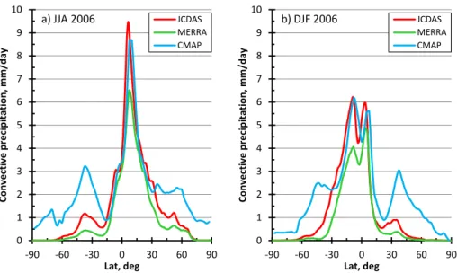
Figure 1 shows zonal mean convective precipitation rates (CP; mm d−1) from the

JRA-25/JCDAS, MERRA and CMAP datasets averaged for June-July-August (JJA) and December-January-February (DJF) 2006. The JRA-25/JCDAS dataset generally

10

captures the latitudinal variation of CP reported in the MERRA and CMAP datasets, although there are large discrepancies among the three datasets in mid-latitudes. The estimates of CP from CMAP and MERRA bracket that from 25/JCDAS. The

JRA-25/JCDAS and CMAP datasets are consistent in shape and only slightly di_fferent in

magnitude in the tropics, whereas the MERRA dataset is biased low compared to the

15

other estimates by 2 mm d−1during both seasons.

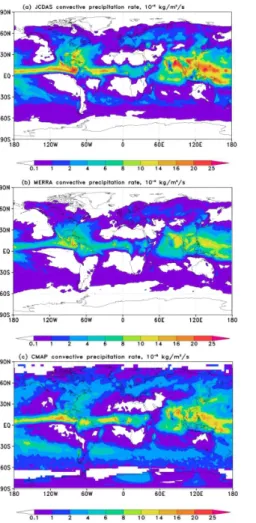
All three datasets indicate seasonal and geographic variations in CP (Table 1). CP is consistently higher in the Northern Hemisphere than in the Southern Hemisphere and also consistently higher during the boreal summer season (JJA) than during boreal winter (DJF). Hot weather during the boreal summer season leads to frequent

convec-20

tive storms in northern temperate latitudes (Fig. 2). The largest amounts of CP occur in equatorial areas and over India and Southeast Asia during the monsoon season (Myoung and Nielsen-Gammon, 2010). The potential for DCC over the ocean persists throughout the night, and convective cells over the ocean commonly reach altitudes in the upper troposphere (Schumacher and Houze, 2003). The seasonal variability of

25

(14)

ACPD

12, 20239–20289, 2012

Title Page

Tables Figures

◭ ◮

Back Close

Full Screen / Esc

Discussion

P

a

per

|

Dis

cussion

P

a

per

|

Discussion

P

a

per

|

Discussio

n

P

a

per

|

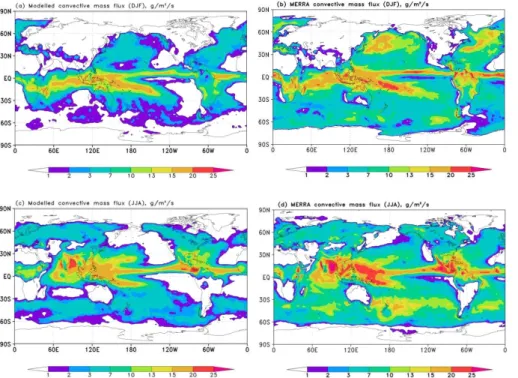
3.2 Evaluation of the simulated convective mass flux

The MERRA special products dataset, which has been developed in conjunction with the chemistry community, provides support for chemistry transport modelling (Wong et al., 2011). This dataset includes a number of meteorological fields that are necessary for tracer transport simulations, including fields that describe convective motion (such

5

as upward convective mass flux). This reanalysis dataset can therefore be used to evaluate simulated convective mass fluxes calculated using Eq. (7).

The convective mass flux calculated by the proposed convection scheme is gener-ally in good agreement with MERRA year-round in the tropics (Fig. 3). This agreement between the two datasets is particularly good over Southeast Asia, the Pacific coast

10

of Central America and the tropical Atlantic Ocean. The proposed convection scheme underestimates convective mass fluxes over the oceanic regions of the western

coast-lines of North and South America, Africa and Australia, and in the Southern Ocean off

the northern coast of Antarctica. The differences over mid-latitude oceanic regions are

larger in both hemispheres during DJF (boreal winter/austral summer) than during JJA.

15

The agreement between the two datasets is better over the continents. Both datasets indicate that convective mass fluxes are fairly evenly distributed over land areas, and discrepancies in the simulated intensity of convective mixing are much lower.

Convective precipitation rates in the JRA-25/JCDAS dataset used to drive the model and the MERRA dataset agree most closely over the continents and tropical oceans

20

(Fig. 2), exactly where the two convective flux datasets agree. The regional mismatches in intensity described above indicate that convective precipitation does not always ac-company upward convective mass flux; nevertheless, the proposed convection scheme successfully captures most of the large-scale upward convective mass flux that is ac-companied by convective precipitation. The method does not appear to reproduce

up-25

ward fluxes at smaller scales.

(15)

ACPD

12, 20239–20289, 2012

Title Page

Tables Figures

◭ ◮

Back Close

Full Screen / Esc

Discussion

P

a

per

|

Dis

cussion

P

a

per

|

Discussion

P

a

per

|

Discussio

n

P

a

per

(Lawrence and Salzmann, 2008). It is therefore necessary to further evaluate the pro-posed method using tests that consider the full spectrum of processes that influence vertical transport.

4 Validation of the parametrisation using222Rn

As global simulations of the short-lived tracer 222Rn provide a very efficient means

5

of evaluating convective parametrisations in this section, the output of the NIES TM outfitted with the proposed convection scheme is compared with observational data

and the output of TransCom-CH4transport models.

4.1 Intercomparison with TransCom-CH4transport models

Observational measurements of 222Rn are currently sparse and insufficient to

ade-10

quately define global and regional radon profile climatologies. It is therefore impossible

to evaluate a cumulus convection parametrisation in different latitudinal zones using

observations alone. In this study, the output of the NIES TM with the proposed con-vection scheme is compared with the results of radon simulations performed by other

transport models during the TransCom-CH4 TMI. We should note that the version of

15

NIES TM considered here with the deep cloud parametrisation scheme described in

Sect. 2 is similar to the model that participated in the TransCom-CH₄intercomparison,

which covers the period 1990–2007.

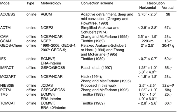
The eleven additional CTMs that participated in the TransCom-CH4 TMI and

simu-lated222Rn fields include the Australian Community Climate and Earth-System

Simu-20

lator (ACCESS; Corbin and Law, 2011), the Atmospheric general circulation model-based CTM (ACTM; Patra et al., 2009), the Community Atmosphere Model (CAM; Gent et al., 2009), CSIRO Conformal-cubic Atmospheric Model (CCAM; Law et al., 2006), Goddard Earth Observing System Chemical transport model (GEOS-Chem; Fraser et al., 2011), The ECMWF Integrated Forecast System (IFS; Bechtold et al.,

(16)

ACPD

12, 20239–20289, 2012

Title Page

Tables Figures

◭ ◮

Back Close

Full Screen / Esc

Discussion

P

a

per

|

Dis

cussion

P

a

per

|

Discussion

P

a

per

|

Discussio

n

P

a

per

|

2004; http://www.ecmwf.int/research/ifsdocs/CY36r1/index.html), the Integrated Mas-sively Parallel Atmospheric Chemical Transport (IMPACT; Rotman et al., 2004), Model for OZone And Related chemical Tracers version 4 (MOZART; Emmons et al., 2010), the Goddard Space Flight Center Parameterized Chemistry and Transport Model (PCTM; Kawa et al., 2004), the Transport Model 5 (TM5; Krol et al., 2005) and the

5

TOMCAT CTM (Chipperfield, 2006) models (Table 2).

Four of the model simulations were run in online configurations (ACCESS, ACTM

CCAM and IFS) while the remaining models were run in offline configurations The

Tiedtke (1989) parametrisation scheme is used in four of the models (CCAM, IFS, TM5 and TOMCAT) and the Zhang and McFarlane (1995) parametrisation scheme is used

10

in three (CAM MOZART and PCTM). The horizontal resolutions range from 0.7◦×0.7◦

to 6◦×4◦ (longitude×latitude), and the number of vertical levels varies from a low of

18 to a high of 67 (see Table 2).

The comparison of the NIES and PCTM transport model is very useful, as the PCTM model is unique in supporting this dynamical convection study (Sect. 3) because it

15

uses NASA GEOS-5 MERRA to perform the TransCom-CH4simulation for the whole

18 yr. Therefore, the PCTM results facilitate the study of MERRA dynamic fields in conjunction with cloud and precipitation analyses.

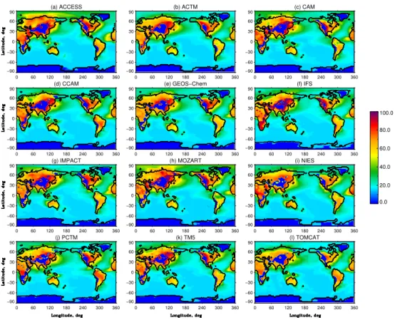
4.2 Geographical distribution of222_Rn

The modelled distributions of mean radon concentrations at 900 hPa are very

hetero-20

geneous (Fig. 4). The highest concentrations are located over the continents, with

mag-nitudes of 800–1000×10−21mol mol−1during January and 600–800×10−21mol mol−1

during July. Radon concentrations are very low over open oceans, consistent with the low emissions in these regions. Concentrations near coastal regions are slightly higher due to the greater influence of land emissions. Filaments of high radon concentration

25

(17)

ACPD

12, 20239–20289, 2012

Title Page

Tables Figures

◭ ◮

Back Close

Full Screen / Esc

Discussion

P

a

per

|

Dis

cussion

P

a

per

|

Discussion

P

a

per

|

Discussio

n

P

a

per

into upper layers (Fig. 4). Both vertical mass transport and the global redistribution of mass between hemispheres are more intense during summer than during winter. This seasonal variability plays a large role in determining the alignment of the concentra-tion field, leading to the absence of strong peaks in northern temperate latitudes and producing minima over Antarctica.

5

Among the considered models, ACCESS, CAM, GEOS-Chem, IMPACT, MOZART

appear to be more diffusive, as they show relatively high radon concentration over the

Arctic ocean in January (Fig. 4).

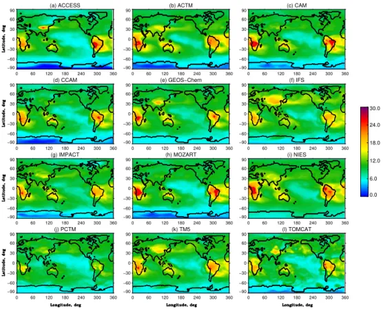
At 300 hPa, the radon concentration depends strongly on atmospheric stability and the intensity of vertical transport (Fig. 5). The highest radon concentrations at 300 hPa

10

are found over tropical Africa and South America year-round and over Southeast Asia especially during the summertime rainy season (not shown). The locations of these maxima are consistent with the locations of the most intense convective updrafts and

the land sources of 222Rn. Throughout the atmosphere, the lowest 222Rn

concentra-tions are year-round over the tropical Pacific Ocean. This minimum is associated with

15

powerful convective updrafts pumping “clean” air upward from the boundary layer to the tropopause. Seasonal variations at 300 hPa are generally smooth, and are most prominent in northern temperate latitudes.

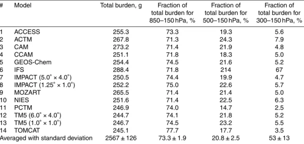
We analyzed total, middle and upper tropospheric (from the 850, 500 and 300 hPa

levels to the tropopause)222Rn burdens averaged over one year (Table 3). The mean

20

total burden averaged using data from 14 model versions (low and high resolution versions of IMPACT and TM5 were considered) is about 256 g, that is about 20 % larger than was estimated by Tost et al. (2010) for ECHAM5/MESSy.

As most of the atmospheric 222Rn is located in the troposphere, 26 % of the222Rn

burden is found below 850 hPa, 80 % below 500 hPa and more than 95 % below

25

300 hPa. The smallest total burdens are found in PCTM, TM5 and TOMCAT. Relatively large burdens are found in ACTM, CAM, IFS and MOZART.

Fractions of the total burden for ACCESS, CAM, GEOS-Chem IFS, IMPACT

(18)

ACPD

12, 20239–20289, 2012

Title Page

Tables Figures

◭ ◮

Back Close

Full Screen / Esc

Discussion

P

a

per

|

Dis

cussion

P

a

per

|

Discussion

P

a

per

|

Discussio

n

P

a

per

|

cases. Among the considered models ACTM, IMPACT (1.25◦×1.0◦), NIES and TM5

(1.0◦×1.0◦) show the strongest penetrative mass flux due to deep cumulus

convec-tion, and PCTM and TOMCAT relatively weaker.

The higher horizontal resolution versions of both IMPACT and TM5 resulted in higher 222

Rn concentrations above 500 hPa compared to their respective lower resolution

sim-5

ulations. The use of a high-resolution grid leads to a more detailed description of con-vective processes in the upper troposphere (Patra et al., 2011).

4.3 Zonal mean radon concentration

Patra et al. (2011) analysed the zonal mean concentrations of radon simulated by the

TransCom-CH4models. For instance, they used the simulated

222

Rn distributions over

10

the South Asian monsoon region (70◦E) during boreal summer.

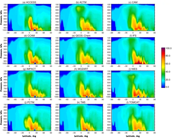
This study focuses on 222Rn distributions over the oceanic regions of the western

coastlines of Africa (0◦–30◦S, 5◦E), where the proposed convection scheme

underes-timates convective mass fluxes in comparison to MERRA (Sect. 3.2). Significant222Rn

emissions occur north of the equator along 5◦E longitude where land occurs, while

15

emissions are much smaller over the ocean to the south of the equator. The combi-nation of the emission and powerful year-round convection results in strong vertical

transport of222Rn throughout the year over 15◦S–4◦N (Fig. 6). This vertical transport

extends upward to 100–200 hPa in the upper troposphere. The location of the most in-tense convective transport fluctuates northward during boreal summer and southward

20

during boreal winter, following the inter-tropical convergence zone (not shown). The

NIES TM and ACTM produce notable areas of enhanced222Rn concentrations in the

tropical upper troposphere between 200 and 300 hPa (Fig. 6).

The lowest concentrations are located over the ocean (15◦S–70◦S) and Antarctica

(Fig. 6). Convective transport over Africa induces a steep gradient in radon

concen-25

trations throughout the troposphere south of 15◦S, especially during boreal winter, as

(19)

ACPD

12, 20239–20289, 2012

Title Page

Tables Figures

◭ ◮

Back Close

Full Screen / Esc

Discussion

P

a

per

|

Dis

cussion

P

a

per

|

Discussion

P

a

per

|

Discussio

n

P

a

per

Thus, from comparison with the TransCom-CH₄ models we found no problems with

the222Rn distributions calculated by NIES TM over regions with weak convective mass

fluxes (0◦–30◦S, 5◦E) (Fig. 6). Apparently, insufficient reproduction of small-scales

con-vective fluxes in this area is compensated by concon-vective activity in adjoining regions and other transport processes e.g. turbulent mixing and large-scale wind dynamics.

5

4.4 Comparison of model results with observed vertical profiles

In this section, the ability of the model simulations to capture the vertical structure of

radon is evaluated using observations. Vertical profiles of 222Rn mixing ratios in the

troposphere are available from aircraft observations (Liu et al., 1984; Zaucker et al., 1996; Kritz et al., 1998); however, the times at which these observations have been

10

performed does not always overlap with the meteorological data used to drive the mod-els. Patterns of advection can exert a large influence on the distribution of radon in the

atmosphere. To limit weather-related differences, the validation is performed using only

those composites of observational data that represent long-term (seasonal or annual) regional mean estimates of the vertical distribution of radon (Mahowald et al., 1995).

15

The set of summer and winter profiles for the Northern Hemisphere compiled by Liu et al. (1984) meets these criteria. Mean profiles are calculated for the period 1950– 1972 at a variety of continental locations. The winter (DJF) mean profile includes data from seven sites, and the summer (JJA) mean profile includes data from 23 sites.

Pro-files of radon obtained in the free troposphere obtained near Moffet Field, California

20

(37.5◦N, 122.0◦W) during the period 3 June–16 August 1994 (Kritz et al., 1998) are

used in an independent comparison. These profiles extend from the surface to 11.5 km

altitude, with typical measurement errors of ∼6 %. Measurements from nine flights

associated with the North Atlantic Regional Experiment (NARE) during August 1993 (Zaucker et al., 1996) are used in a third independent comparison. These

observa-25

tions were taken over the North Atlantic Ocean and between Nova Scotia and New Brunswick in Eastern Canada. Profiles of radon were taken from the surface to 5.5 km

(20)

ACPD

12, 20239–20289, 2012

Title Page

Tables Figures

◭ ◮

Back Close

Full Screen / Esc

Discussion

P

a

per

|

Dis

cussion

P

a

per

|

Discussion

P

a

per

|

Discussio

n

P

a

per

|

Figure 7 shows vertical profiles of 222Rn over land areas in the mid-latitudes and

tropics during the DJF and JJA seasons. The mean observational profiles compiled by Liu et al. (1984) are included in the panels corresponding to mid-latitude land ar-eas in the Northern Hemisphere (Fig. 7a, b). The structure of the observed summer and winter profiles is approximately piecewise in three sections. Radon concentrations

5

initially decrease at an approximately log-linear rate from the surface to 600 hPa. This rate of decrease is reduced between 600 and 250 hPa and enhanced in the upper troposphere. During summer, the proposed convective scheme successfully captures the lower and middle components of this structure Cold weather during winter in the Northern Hemisphere inhibits the development of convection over land so that

convec-10

tive precipitation rarely occurs (Fig. 3a). These conditions lead to a steep gradient in the mean vertical profile of radon concentration during this season, with a minimum in the middle atmosphere between 800 and 400 hPa (Fig. 7a). All model profiles appear

to be more uniform below∼850 hPa than the observations.

Figure 8 presents profiles of222Rn concentration over two coastal regions. The first

15

region is near Moffett Field in California, USA (Fig. 8a); simulated profiles in this region

are averaged over the month of June for comparison with the observed profiles initially

presented by Kritz et al. (1998). The second region is offthe eastern coast of Canada

(Fig. 8b); simulated profiles in this region are averaged over the month of August for comparison with the observed profiles initially presented by Zaucker et al. (1996).

20

The simulated vertical structure of 222Rn at Moffett Field during June corresponds

well to the observed mean profile below 200 hPa. The discrepancy between model and observations above 200 hPa was also seen by Zhang et al. (2008). Feng et al. (2011) suggested that GCMs generally underestimate the vertical extent of tropical convec-tion, including mean cloud top height and convective mass fluxes in the upper most

25

troposphere. The proposed convective parametrisation slightly overestimates the con-centration of radon at the tops of convective cells because it overestimates organized

(21)

ACPD

12, 20239–20289, 2012

Title Page

Tables Figures

◭ ◮

Back Close

Full Screen / Esc

Discussion

P

a

per

|

Dis

cussion

P

a

per

|

Discussion

P

a

per

|

Discussio

n

P

a

per

rapidly above this level because of the implementation of isentropic vertical coordi-nates, which inhibits the transport of tracers into the stratosphere (Belikov et al., 2012).

The results of the proposed convective scheme agree well with observations of222Rn

taken in the lower part of the troposphere during the NARE aircraft campaign (Fig. 8b).

The observations are unavailable above 6 km. The various models produce di_fferent

5

profiles of radon concentration above this level; consequently, it is not currently possible to adequately validate the results of the convective parametrisation in this region.

The proposed convective parametrisation generally produces vertical profiles of radon concentration that are consistent with physical expectations. The vertical pro-files simulated by the proposed parametrisation agree reasonably well with both

obser-10

vational measurements and vertical profiles simulated by the TransCom-CH₄models.

In general, simulated radon mixing ratio decreases at a lower altitude in PCTM and TOMCAT compared to the other models.

4.5 Comparison of model results with surface measurements

The simulated surface222Rn concentrations are validated against in situ surface

mea-15

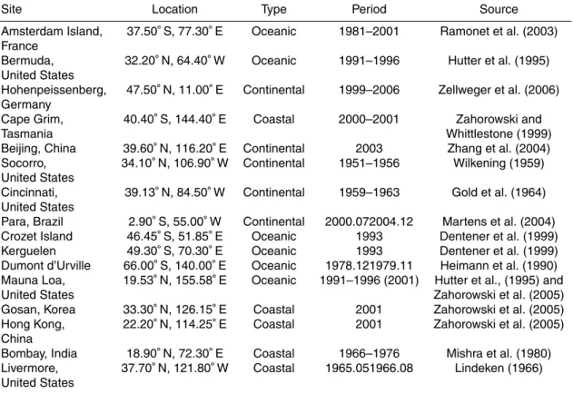
surements by interpolating model output to the spatial coordinates and altitude of the observations. Simulated and observed time series of monthly mean concentrations of radon at four sites are shown in Fig. 9 (Feng et al., 2011), and simulated and ob-served seasonal cycles of radon at 12 sites are summarized in Fig. 10 (Zhang et al., 2008). Basic information about these measurements is presented in Table 4. Radon

20

concentrations are reported in units of millibecquerel per cubic meter at standardized

temperature (273.15 K) and pressure (1013.25 hPa) (mBq m−3STP).

4.5.1 Comparison with continuous measurements of222_Rn

The models are able to reproduce monthly mean variations in radon concentrations at a variety of surface sites (Fig. 9). This agreement between simulations and

obser-25

(22)

ACPD

12, 20239–20289, 2012

Title Page

Tables Figures

◭ ◮

Back Close

Full Screen / Esc

Discussion

P

a

per

|

Dis

cussion

P

a

per

|

Discussion

P

a

per

|

Discussio

n

P

a

per

|

radon at the surface. Good results are obtained at the oceanic sites Amsterdam Island

and Bermuda (Fig. 9a, b), since these sites are mainly affected by large-scale transport

(Zhang et al., 2008). All of the models overestimate summer concentrations of222Rn at

Amsterdam Island (Fig. 9a). We should note, the apparent change in behaviour from poor simulations from 1994–1998 to better ones later.

5

Similar to the results presented by Zhang et al. (2008) and Feng et al. (2011), the model simulations evaluated in this paper show large discrepancies at the continen-tal European station Hohenpeissenberg (Fig. 9c). Complicating factors in the

model-measurement comparison include the strong dependence of observed surface222Rn

on the structure of the boundary layer, the coarse horizontal resolution of the models

10

and the possible errors in estimation of local emissions in the222Rn fluxes used in the

simulations (Jacob et al., 1997). We have to note that the observed concentration data

have high scatter about 2.0–2.5 Bq m−3. The majority of the models are successful in

reproducing the monthly variations at Cape Grim (Fig. 9d). The exception is ACCESS. As a coastal site, the monthly variations are determined by meteorology (i.e. the

pro-15

portion of time that air reaching the site is oceanic or continental in origin). ACCESS is unable to capture this variation since its transport is not nudged to analyses.

4.5.2 Comparison with observed seasonal variations

Figure 1 shows the seasonal variation of 222Rn concentrations at continental sites

(Fig. 1a–d), remote island sites (Fig. 1e–h) and coastal sites (Fig. 1i–l). We also

ana-20

lyzed model-observation correlations, to obtain a quantified characteristic of the mod-els performance (Fig. 11), despite high modmod-els biases and small seasonal cycle of the tracer.

The models qualitatively reproduce seasonal variability in radon concentration in Bei-jing (Fig. 1a), but the amplitude of this variability is severely underestimated. Zhang

25

(23)

ACPD

12, 20239–20289, 2012

Title Page

Tables Figures

◭ ◮

Back Close

Full Screen / Esc

Discussion

P

a

per

|

Dis

cussion

P

a

per

|

Discussion

P

a

per

|

Discussio

n

P

a

per

suggests that the model simulations may also properly characterize the annual mean concentration in Beijing.

Socorro (Fig. 1b) and Cincinnati (Fig. 1c) are mid-latitude sites with features similar to those observed in Beijing. The models are only able to reproduce observed concen-trations at Socorro during the summer season, likely because the models are unable

5

to capture the strong seasonal changes in wind direction and boundary layer depth that occur at Socorro. All models except ACTM show a negative correlation for Socorro (Fig. 11). Cincinnati is located in a transition zone between a humid subtropical climate

and a humid continental climate. The model simulations clearly underestimate 222Rn

concentrations in Cincinnati during August–October (Fig. 1c).

10

At the Para station (Fig. 1d), radon observations are collected on a tower and include measurements taken both within and above the forest canopy (ranging between 32 m and 61 m a.g.l.). The average measured concentration is quite high due to the lack of

turbulent mixing in the canopy layer. Probably a mix of effects is seen in the model-data

comparison: boundary layer stability, turbulent mixing as several models underestimate

15

the concentration of222Rn at Para. The climate at Para is typical of a tropical rainforest,

resulting in small seasonal variations in radon concentrations. Correlations are quite mixed between models.

Concentrations of radon at isolated oceanic sites are affected primarily by large-scale

transport rather than immediate emission and local circulation; it is therefore expected

20

that simulated seasonal cycles of radon concentrations in these regions should match observations better than those in continental regions. Sites located in oceanic regions are characterized by much lower concentrations than continental sites, consistent with lower levels of emission (Fig. 1e–h).

Crozet (Fig. 1e) and Kerguelen (Fig. 1f) are located at high latitudes in the

South-25

(24)

ACPD

12, 20239–20289, 2012

Title Page

Tables Figures

◭ ◮

Back Close

Full Screen / Esc

Discussion

P

a

per

|

Dis

cussion

P

a

per

|

Discussion

P

a

per

|

Discussio

n

P

a

per

|

transport. The high concentrations of radon in this long-range transport likely originate in the southern regions of South America and Africa, as the prevailing winds at these sites are westerly year-round. Dentener et al. (1999) pointed out that positive biases in

simulated222Rn concentrations at Crozet and Kerguelen result from overestimates of

emission from South America during austral winter months (i.e. frozen soil treated as

5

non-frozen). Biases at these two sites should therefore not be considered as defects in the numerical models, but as limitations in the experimental design (Zhang et al.,

2008). All models except TM5 can reproduce seasonal cycle (r ¿ 0.5) (Fig. 11).

The observed seasonal cycle of radon concentrations at Dumont d’Urville (Fig. 1g) is similar to the seasonal cycles at Crozet and Kerguelen, but the annual maximum

10

occurs during austral summer rather than during austral winter. The positive biases in simulated concentrations between June and September have the same origin as the positive biases in simulated concentrations at the Southern Ocean stations during these months. The simulations assume that emission in these regions is zero year-round. A negative or small correlation is found for all models (Fig. 11).

15

The Hawaiian islands are large enough to produce non-negligible local radon emis-sions, but too small to be resolved by global CTMs (Zhang et al., 2008). Incorrect radon source information is also culpable for the systematic low biases in simulated concen-trations at Mauna Loa (Fig. 1h), while models performance in reproducing seasonality

is good (r ≈0.5–0.8).

20

Figure 1i–l shows simulated and observed seasonal cycles at coastal sites.

Sur-face222Rn concentrations at coastal sites represent the complicated set of processes

that occur in transitional zones between large continents and oceans. The accuracy of a simulated seasonal cycle of radon concentration in a coastal area therefore depends strongly on the ability of the model to realistically represent seasonal contrasts in wind

25

direction and reproduce the detailed circulation in a relatively small region surrounding the site.

(25)

ACPD

12, 20239–20289, 2012

Title Page

Tables Figures

◭ ◮

Back Close

Full Screen / Esc

Discussion

P

a

per

|

Dis

cussion

P

a

per

|

Discussion

P

a

per

|

Discussio

n

P

a

per

reproduce the observed seasonal cycle (r≈0.5–0.9). The simulated seasonal cycles

at Livermore on the west coast of North America (Fig. 1l) is less successful (only half of the models reproduce the seasonal cycle).

Simulated seasonal cycles in 222Rn concentrations generally match observed

sea-sonal cycles at continental, oceanic and coastal sites. The strength of vertical transport

5

for some sites is overestimated by ACTM, which accordingly underestimates 222Rn

concentrations. At the same time, the results of this model show better agreement with the observed seasonal cycle By contrast, IMPACT appears to be the model that over-estimates concentrations. Outfitting the NIES TM with the proposed parametrisation scheme produces seasonal cycles similar to those simulated by TM5, but with higher

10

amplitudes at Crozet, Kerguelen, Dumont and Bombay. Like the majority of the

mod-els considered in this analysis, NIES TM tends to overestimate222Rn at oceanic sites

and is unable to successfully reproduce the complicated seasonal cycles at continental sites. However, the model agrees well with observations at coastal areas.

5 Discussion

15

In this work, we presented the modified cumulus convection parametrisation scheme, which computes the mass of air transported upward in a cumulus cell using conser-vation of moisture and a detailed distribution of convective precipitation provided by a reanalysis dataset. This approach is more straightforward, than the original Kuo-type scheme which integrates the total horizontal moisture convergence to calculate updraft

20

mass flux, because the new scheme does not involve additional spatial and tempo-ral interpolations between the reanalysis model grid, the reanalysis data grid and the transport model grid. Moreover, the modified scheme is more flexible, as it is able to

use convective precipitation data from different reanalysis.

The proposed convective scheme can successfully reproduce deep cloud

convec-25

(26)

ACPD

12, 20239–20289, 2012

Title Page

Tables Figures

◭ ◮

Back Close

Full Screen / Esc

Discussion

P

a

per

|

Dis

cussion

P

a

per

|

Discussion

P

a

per

|

Discussio

n

P

a

per

|

The proposed convection scheme underestimates the convective mass flux across

significant areas (Fig. 3). The modeled convective rain rate is very di_fferent in di_fferent

reanalysis datasets (Table 1, Figs. 2–3) as it highly depends on the convection scheme

used the model resolution and other model features. Therefore, it is difficult to know

how much of the error shown in this work is due to the reanalysis product chosen and

5

how much is due to the new convection scheme itself.

This model version employs a hybrid sigma–isentropic (σ–θ) vertical coordinate

con-sisting of terrain-following and isentropic levels switched smoothly near the tropopause. Vertical transport in the isentropic part of the grid in the stratosphere was controlled by

an air-ascending rate derived from the JRA-25/JCDAS reanalysis effective heating rate

10

(Belikov et al., 2012). Due to such vertical coordinate NIES TM has more limited vertical transport in the upper troposphere/lower stratosphere region than every other model. As a result, the model with the new scheme has larger concentrations in the Northern Hemisphere above 200 hPa (Fig. 6) and overestimates the concentrations in the levels between about 400–100 hPa and then underestimates them above (Fig. 7).

15

To perform the TransCom-CH4simulation for the whole 18 yr the PCTM model uses

NASA GEOS-5 MERRA reanalysis, which we used to study dynamical convection (Sect. 3) and evaluate convection mass flux calculated in NIES TM. The convection

scheme of PCTM used for Transcom-CH4activity is a semi-implicit convection module

(i.e. CONV1 in Bian et al., 2006), constrained by the total convective mass flux (CMF)

20

from MERRA, in which air parcels entrained at cloud base are transported upwards, detraining at a rate proportional to the convergence of MERRA CMF (Kawa et al., 2004).

It is worth noting that the convective transport algorithm used in the PCTM

Transcom-CH4study uses only the total net cloud flux of MERRA to solve a layer’s mean mixing

25