Temperature Control of Continuous Chemical Reactors Under Noisy Measurements and Model Uncertainties

Vol. 10, June 2012 

428 

 

Temperature Control of Continuous Chemical Reactors Under Noisy

Measurements and Model Uncertainties

Ricardo Aguilar López*1, Rafael Martínez Guerra2, Juan L. Mata Machuca3 1

Departamento de Biotecnología y Bioingeniería 2

Departamento de Control Automático CINVESTAV-IPN

Av. I.P.N. No. 2508, San pedro Zacatenco, México, D.F. C.P. 07360, MEXICO *raguilar@cinvestav.mx

ABSTRACT

The aim of this paper is to present the synthesis of a robust control law for the control of a class of nonlinear systems named Liouvillian. The control design is based on a sliding-mode uncertainty estimator developed under the framework of algebraic-differential concepts. The estimation convergence is done by the Lyapunov-type analysis and the closed-loop system stability is shown by means of the regulation error dynamics. Robustness of the proposed control scheme is tested in the face of noise output measurements and model uncertainties. The performance of the proposed control law is illustrated with numerical simulations in which a class of oscillatory chemical system is used as application example.

Keywords: I/O linearizing controller, sliding-mode observer, uncertainty estimation, noisy measurements.

RESUMEN

El objetivo de este artículo es presentar la síntesis de una ley de control robusta para una clase de sistemas no lineales denominados Liouvilianos. El diseño de control esta basado en un estimador de incertidumbres de modos deslizantes, desarrollado bajo el enfoque de conceptos algebraico-diferenciales. La convergencia del estimador se realiza mediante el método de Lyapunov y la estabilidad del sistema en lazo cerrado se demuestra mediante la dinámica del error de regulación. La robustez del esquema de control propuesto se determina tomando en cuenta la presencia de ruido en la salida del sistema e incertidumbres en el modelo. El desempeño de la ley de control propuesta se ilustra con simulaciones numéricas, donde se considera una clase de sistema químico oscilatorio como ejemplo.

   

1. Introduction

Since the early 1990s, some papers have been related with the dynamic characterization of a particular class of nonlinear systems named differentially flat [1,2] and Liouvillian systems [3], based on the frame of differential algebra. One of the most important aspects of this approach for this kind of systems is the explicit relationship that can be obtained for particular state variables; it is an advantage for a class of observation and control problems. Differential-algebra based techniques have been employed for differential algebraic as well as ordinary differential equations systems. On the other hand, control of non-linear systems has been widely studied during the last 20 years, specially the characterization of input/output (I/O) and exact linearizable systems. This corresponds to systems that can be fully or partially linearized by

Journal of Applied Research and Technology ₄₂₉ when the knowledge of the nonlinearities is very

poor or null such that conventional linearizing techniques are inadequate. In the face of these events, the robust stability problem for uncertain systems arises as a necessary control design approach to supply the controller with the corresponding on-line information and try to realize a satisfactory closed-loop performance. Research on robust control design for linearizable nonlinear systems has been done considering observer-based controllers [6] where peaking phenomena, stability issues and robust performance are still topics that deserve further study.

In recent works, it has been employed Luenberger-type observer structures to obtain on-line estimates of uncertain signals [7]. However, the resulting schemes become sensitive to measurement noise. Since measurement noise is propagated through the control loop, high frequency chattering can induce premature degradation of actuator (e.g., valves) components. In this paper, a design of robust control law based on on-line uncertainty estimation is addressed; the robustness is referred to model uncertainties and noisy output measurements. The uncertainty estimator contains a sliding-mode structure and it is designed within the framework of algebraic theory. Subsequently, the uncertainty estimator is coupled with an input-output linearizing controller, which produces practical stability (i.e., the closed-loop trajectories are forced to remain in a neighborhood of the operating equilibrium point). The performance of the robust control design is illustrated via numerical simulations.

2. Main definitions

The framework of the observer design for control purposes is based on capturing the input-output behavior of the system employing a set of

equations generated by the system under study. The definitions presented in this section have been discussed previously in [8] and are summarized below for completeness.

Definition 1. A dynamics is defined as a finitely generated differentially algebraic extension

H/k<u> of the differential field k<u>, where k<u>

denotes the differential field generated by k and elements of a finite set u = (u1,u2,…,un) of

differential quantities.

Definition 2. A differential transcendence basis y = (y1,y2,…,ym) of H/k such that H = k<y> is called

linearizing or flat output of the system H/k.

Definition 3. The number of state variables, not permissible in terms of the flat outputs, is known as the defect of the non-flat system, that is, the integer number, which does the differential transcendence degree of H/k is minimal, is called algebraic defect of the system.

Definition 4. A system H/k is differentially flat if and only if its defect is zero. If its algebraic defect is non-zero, then the system H/k is said to be differentially non flat.

Definition 5. Let H/k be a given system and let M be such that k  M  H. Moreover, it is assumed that

M/k is a flat subsystem of H/k, and then it can be said that H/k is Liouvillian if the elements of H - M can be obtained by an adjunction of integrals or exponential of integrals of elements of the flat field M.

2.1 Example

Now, consider the following generic mathematical model of a class of continuous chemical reactors, wher the following chemical reaction is considered:





₂

1

x

x

Prod

 Mass Balance for reactive 1 (x1):

(a)



 



_









 











3 2

1 1 3

2 1 1

1

,

,

exp

x

x

x

x

a

x

x

x

f

Temperature Control of Continuous Chemical Reactors Under Noisy Measurements and Model Uncertainties,Ricardo Aguilar López et al. / 428‐446 

Vol. 10, June 2012  430 

 Mass Balance for reactive 2 (x2):

(b)  Energy Balance (x3):

(c)

 Measured output:



0

0

1







C

x

where

C

y

(d)

The above system will be expressed via differential-algebraic tools, based on the definitions given in Section 2, as a set of mapping in the variables xi, y and u, which will be considered to describe the

input-output behavior in the system and it is below used in the observer design procedure.

From system (a)-(d), and after algebraic manipulation, the following expressions are generated:  Reactive 1

(e) Where:

 Reactive 2:

(f)  Temperature:

(g)

As can be observed H = k<x1, x2, x3, u>, k = , the reactor model (a)-(d) is a nonlinear Liouvillian system,

besides note that the state variables of the reactor x1 and x2 are observables from temperature

measurements.



 



_









 











3 2

1 2 3

2 1 2

2

,

,

exp

x

x

x

x

a

x

x

x

f

x







 





3



3 2

1 3

3 2 1 3

3

,

,

exp

u

x

x

x

x

d

x

b

x

x

x

f

x

_













 

















 

y

u



a



t



 

h

y

t

u



dt

g

x

₁



₁

,





exp





₁

(

),

 



 









































a

d

y

b

y

u

y

u

y

h

₁

,

 



 



 

 

a

dt

y

u

y

g

d

y

u

y

g

a

y

b

y

u

y

u

y

g

x











































 











 















_

_

_

_

















exp

,

exp

,

,

1 1 2

2

 

y

u

y

g

Journal of Applied Research and Technology ₄₃₁

3. Problem statement

Non-linear approaches to design control laws have been tested successfully in theoretical research. In particular, the I/O linearizing technique shows attractive characteristics for the control of the non-linear systems.

To motivate the control problem, consider the following non-linear Liouvillian system, which represents the general mathematical model of a continuous stirred tank reactor (CSTR):



1 1



(

1

,

2

)

1

x

x

ER

x

x

x



e









(1)



2 2



1 2



2



2

x

x

HR

(

x

,

x

)

u

x

x



e

















(2) where

x

₁ is a n-dimensional vector of chemical species,

R

(

x

₀

,

x

₁

)

is a m-dimensional vector of reaction kinetics,



H

is a m-dimensional vector of reaction enthalpies, E is the stoichiometric matrix,

2

x

is the reactor temperature, u is the cooling jacket temperature, and 1/ and  are the residence time and the heat-transfer global coefficient, respectively. If the reactor temperature

2

x

is the controlled output, in compact form, the Liouvillian system (1)-(2) can be rewritten as follows:

2

2 2

1 2 2

2 1 1 1

)

(

)

(

)

,

(

)

,

(

x

x

h

y

u

x

B

x

x

f

x

x

x

f

x











 

(3)

The zero-dynamics are given by the n-dimensional dynamics of the chemical species concentration at a constant temperature, which are assumed to be locally stable [9]. The study of relative-degree one systems is very important for many control applications, since the dynamics of a wide class of chemical reactors can be described in this form. Such systems are mathematically modeled as

affine systems with respect to the control input [9].

Systems that present relative-degree one display some interesting features, such as the equivalent dissipativeness by means of state or output feedback. In general, it is easier to stabilize

dissipative systems than non-dissipative ones [10]. In what follows, non-linear systems of the form (3) will be considered. In order to stabilize the system defined by Equation (3) via regulation of

x

₂, the following nominal I/O linearizing feedback control is proposed:







3 2 1 2



1 1

2

)

,

(

x

e

f

x

x

B

u





g



 

_

(4) where



_g



0

is a prescribed time-constant. As usual,

e

₃



y



y

_sp and

y

_sp are tracking error and set point, respectively. The controller defined by Equation (4) guarantees asymptotic stability of non-linear systems (3) with no uncertainties and perfect measurements. Moreover, it imposes a linear behavior to the system I/O dynamics by canceling the nonlinearities.

4. Feedback controller design

As it can be noticed, the synthesis of the ideal control law requires accurate knowledge of the mathematical model of the process to be realizable. However, a perfect model is difficult or even impossible to be obtained in practice and, consequently, for uncertain systems, a conventional I/O linearizing controller design is not adequate.

Let us assume that

x

₁ and

x

₂ trajectories are bounded for all

t



0

(i.e., the system is bounded input to bounded output state). The basis of the non-ideal controller design is the nominal control law (4). In order to design the practical robust control law, let us propose the following non-linear dynamic system representation:

2

2 2

2 1 2 2

2 1 1 1

)

(

))

(

)

(

(

)

,

(

)

,

(

x

x

h

y

u

x

B

x

B

x

x

f

x

x

x

f

x















 

Temperature Control of Continuous Chemical Reactors Under Noisy Measurements and Model Uncertainties,Ricardo Aguilar López et al. / 428‐446 

Vol. 10, June 2012  432 

The functions

f

₂

(

x

₁

,

x

₂

)

and



B

(

x

₂

)

are model uncertainties related to the non-linear system, and

)

(

x

B

is a nominal value of the control input coefficient. In the most general case, the functions

)

,

(

1 2 2

x

x

f

and



B

(

x

2

)

are assumed to be unknown. Now, introduce the following function, which corresponds to the I/O modeling error:

u

x

B

x

x

f

u

x

,

)

(

,

)

(

)

(



_{2 1 2}





₂



(6)

By using (6) into (5), a new representation of the system is obtained:

2 2 2

2 1 1 1

)

(

)

(

)

,

(

)

,

(

x

x

h

y

u

x

B

u

x

x

x

x

f

x











 



(7)

Since the uncertainty term,



(

x

,

u

)

, is an unknown function of the states and the control input, the ideal control law for the regulation of

x

₂

is not causal and therefore, it cannot be implemented in practice. Nevertheless, there is another way to develop an input-output linearizing controller that is robust against uncertainties. The procedure described below provides a method to estimate the uncertainty term,



(

x

,

u

)

. Estimators or observers for states and uncertainties can play a key role during the early detection of hazardous and unsafe operating conditions. Motivated by this, much research has focused on the proposition of estimation methodologies for states and uncertainties for monitoring and control purposes [11], [12].

4.1 The uncertainty estimation methodology

Consider the following dynamic subsystem:

2 2 2

)

(

)

,

(

)

(

x

x

h

y

u

x

u

x

B

x













 





(8)

The uncertain term,



(

x

,

u

)

, is considered as a new state and



(

x

,

u

)

is a non-linear unknown function that describes the



-dynamics.

In order to provide a background previous to the proposed estimation methodology, the following definitions are considered [8]:

Definition 6. Let

 

u

,

y

be a subset of  in a

dynamics



/

k

u

. An element in  is said to be

observable with respect to

 

u

,

y

if it is algebraic over

k

u

,

y

. Therefore, a state x is said observable if, and only if, it is observable with respect to

 

u

,

y

.

Definition 7. - An element Xu in  is said to be an

algebraically observable uncertainty if Xu satisfies

a differential algebraic equation with coefficients over

k

u

,

y

.

Now, consider the system (3), which according to Definition 1 defines an algebraic-differential dynamic system. From this subsystem, the following algebraic-differential equations can be obtained:

0

2



y



x

(9)

0

)

(

)

,

(



2







u

x

B

u

x

y



(10)

Remark 1. From Definitions 6 and 7, it follows that the pair (x2, ) is universally observable in the

Diop-Fliess sense 8.

The corresponding Input-Output representation of Equations (9) and (10) can be rewritten in new coordinates as follows:

1 1

 



i_i

i

dt

Y

d

Journal of Applied Research and Technology ₄₃₃

1 2 1 2

2 1

,

,

































 



Y

u

(12)

It should be noted that a partial change of coordinate enables us to estimate 1=y and

2

1









y





(or, equivalently, x2 and



2

x

).

4.2 Measurement output noise considerations

Now, considering the noise case presence:

Y=1+

where  is an additive bounded noise. Our aim is to design an observer to obtain 2 (the uncertainty

term in the transformed space). However, as it can be seen from the nature of the system given by Equation (8), a standard structure of an observer, based on a copy of the system plus measurement error correction is not realizable in this case since the term  is a priory unknown.

4.3 Sliding-Mode Observer

4.3.1 Observer Structure

Proposition 1. The following dynamic system is a

Sliding-mode asymptotic type observer of the system (12) to estimate the variables 1 and 2, respectively:



Y

Y



sign

m

ˆ

ˆ

ˆ

1



2



1



 







, m>0, (13)

_ˆ

m

2 2

sign



Y

Y

ˆ



2





 





, (14)

(15)

and

Now, returning back to the original state space, in view of (6), the heat of reaction can be evaluated as:



2 1

 

1



2

ˆ

ˆ

ˆ

ˆ



















X

_e





u



According to the variable change given by (7), the variable 1 is the thermodynamic reactor temperature (system output). From the above equation for



ˆ

, if temperature measurements are noisy, the noise would be transmitted to the estimation of the heat of reaction that may lead to poor performance in the estimation procedure. That is because it is necessary to filter the temperature measurements. This is the main reason why the structure of the proposed observer (13) - (14) makes sense.

4.3.2 Errors estimation dynamics

Now, let us define the following estimation errors: (16)

(17)

By (12) and (13-14), it follows that the estimation errors e=(e1,e2)T verify the following ordinary

differential equation:

(18)

where:

   

 

  

 



0

m

A ,  > 0 is a regularizing parameter,









ˆ

1

ˆ

Y





























0

)

ˆ

(

0

)

ˆ

(

1

0

)

ˆ

(

1

:

)

ˆ

(

Y

Y

if

undefined

Y

Y

if

Y

Y

if

Y

Y

sign

1 1 1









ˆ

e

m

e

2 2

2

ˆ











Ce



f

Ksign

e

A

e















Temperature Control of Continuous Chemical Reactors Under Noisy Measurements and Model Uncertainties,Ricardo Aguilar López et al. / 428‐446 

Vol. 10, June 2012  434 

     

  _

1 1 1





m m

K , C=[1, 0] and

    

  

   

2 1

1 e m

e

f _



is an uncertainty term (or unmodelled dynamics term).

4.3.3 Main assumptions

A1. There exist nonnegative constants L0f, L1f such

that for any e the following generalized quasi-Lipschitz (strip-bound) condition holds:

A2. The output noise is assumed to be bounded as



_2

:





T







 



 2





where  is a symmetric definite positive matrix playing role of a normalizing matrix (since different components of the output measurements may have a different physical nature).

A3. There exits a positive definite matrix Q0 = Q0 T

> 0 such that the following matrix Riccati equation:

0









A

P

PRP

Q

PA

_ T_

with

R

:





_f1



2



_f

L

_1f

I

,

0





_f





T_f and



L

A



I

Q

Q



₀



2

_1f



_ 2 , has a positive definite solution P = PT > 0.

A4. The gain matrix K is selected as K = kP-1CT where k is a positive constant.

Comment 1. The algebraic Riccati equation in A3 has a positive definite solution if the matrix

A

_ is stable (that is valid for any positive μ) and the following matrix inequality is fulfilled:

In our case this inequality may be transformed to the following one:

e

A

L

L

f



_0f



(

_1f



_

)





_T

 

_T



T

T_{R A Q A R R A R A R R A}

A_ 1 _{ } 1 1 _{ } 1 1 _

4

1    

 _{   }







 



0

1 1 1

1 2

1 1

4

1

2

:

A

R

A

L

A

I

A

R

R

A

R

A

R

R

A

Q

G

T T T

f

T















    

 

 

 

 

Hence, the matrix Q0 providing the existence of the solution to the Riccati equation, always exists if

0





G

.

4.3.4 Lyapunov-type Analysis

Let us define the Lyapunov function candidate V(e) as

(19)

From (15) and using the matrix inequality

valid for any

X

,

Y



R

nm

,

0





_f





Tf, it follows: nxn T T

P

e

Pe

P

P

e

e

V

(

)



2

:



,

0









e



A

e



Ksign



Ce









f







Y

Y

X

X

X

Y

Y

Journal of Applied Research and Technology ₄₃₅







A

e

Ksign

Ce

f



P

e

e

P

e

e

V



(

)



2

T





2

T _













Ce



e

P

f

sign

C

Ke

e

PA

e

T



T T





T





2

_

2



2



PA

A

P



e

Ke

C

sign



Ce



e

P

Pe

 

f

f

e

T



T



T T





T



_f





T



_f





1

2



 



PA

A

P

P

P

Q



e

e

Qe

e

T

f T

T













 



2



L

2_0f





L

_1f



A

_



2

e

2





_f



2

Ke

T

C

T

sign



Ce









PA

A

P

PRP

Q



e

e

Qe

e

T



T







T



_{ } (20)



2



_f

L

2_0f



2

K

 

Ce

T

sign



Ce







The main assumption consists in the implementation of the following inequalities valid for each component:

(21)

Here:

(22) and

(23) The last results from the Cauchy-Bounyakowski-Schwarz inequality:

(24)

for

a

_i

:



n

1

,

b

_i

:



z

_i . Applying (21) to (20) and taking into account A3, it follows:

V



(

e

)





e

T

Qe



2



_f

L

2_0f



2

K

 

Ce

T

sign



Ce







 



_







 















n

i i

f f T

n

Ce

K

L

Qe

e

1 2

0

2

2

2



 

)

(

2

1

K

Ce

K

Qe

e

n

i i

T



_









 (25)



 





















   





























n

i

n

i

n

i

n

i i i

i i

n

i

i

T T

T

z

n

x

z

x

z

z

x

z

x

sign

z

z

x

sign

z

x

z

x

sign

x

1 1 1 1

1

2

2

)

(



x



z



i



x

i



z

i







n

i

i

n

z

z

1







  



n

i

n

i i n

i i i

i

b

a

b

a

1 1

2 1

Temperature Control of Continuous Chemical Reactors Under Noisy Measurements and Model Uncertainties,Ricardo Aguilar López et al. / 428‐446 

Vol. 10, June 2012  436 

where



(

K

)

:



2



_f

L

2_0f



4

K

n



1



. (26)

Since







T



1/2



1



1/2







1



T









1



2_ and

 

Ce

n

 

 

Ce

Ce

CP

P

e

_P

e

T

Q

e

i n

i i



























 

2 2 / 1 2 / 1 2

1 2 2

1

(27)

with

:

2

0

1 2

1

min

















P



C

T

CP



P





.

Then, (25) implies

 

e

e

K

e

 

K

dt

d

e

V

(

)



_P





_Q



2



P





2 2

















Q

V

(

e

)

V

(

e

)

(28)

where

:

2

0

1 2

1

min

















P



Q

T

QP



Q





,



:



2

K



_P, and



:





(

K

)

.

At this point we are ready to formulate the main result.

Theorem 1. If the assumptions A1 - A3 are satisfied then

(29)

where

 

 





 

2

2

:

~

~

























P Q

P

K

K

K

K

K















, and the function

 



_ is defined as



4.3.5 Proof of Theorem 1

Consider the Lyapunov function V(e) verifying the differential equation:

The equilibrium point V* of this equation, satisfying ,

0

~

1









 



V



 















0

0

0

:

Z

if

Z

if

Z

Z

















V

V

V

0







Journal of Applied Research and Technology ₄₃₇ Defining



:





V



V

*



2. The time derivative is given by:





































2

V

V

*

V



2

V

V

*

V

V



2



V



V

*









V





V











V

*





V

*











2



V



V

*

 







V



V

*









V



V

*









2





V



V

*



2



2





V



V

*



V



V

*



2



0

for any V V*, that implies:

lim

V

V

*

t



. For

we obtain:

The last inequality implies that Gt converges, that is,

The integration of the last inequality from 0 to t yields















_

 

_

















t t

d

V

V

V

V

V

V

G

G

0 0

*

*

~

1

2









That leads to the following inequality

Dividing by t and taking the upper limits of both sides, we obtain:

li

m

1

1

~





*





*





0

0















 



 



t

t

_t

V

_V



V

V



V

V

d









2 2

~

2

1

~

:











 







V

V

V

G























*

*



0

~

1

2

~

1

2

~

1

2

~

2

:















 

















 









 







 



 

 

V

V

V

V

V

V

V

V

V

V

V

V

V

V

V

G

t

























G

*

G

t

































 



t

t

G

G

G

d

V

V

V

V

V

V

0

0 0

*

*

~

1

Temperature Control of Continuous Chemical Reactors Under Noisy Measurements and Model Uncertainties,Ricardo Aguilar López et al. / 428‐446 

Vol. 10, June 2012  438 

and there exists a subsequence tk such that:













0

0 * *

~ 1

 





 

  

      



k t

t t

t t

k

k k

k k

G

V V V

V V

V







Hence, it follows that G* = 0; that is equivalent to the fact:

The theorem is proven.

Remark 2. Theorem 1 actually states that the weighted estimation error converges to the zone



~

asymptotically, that is, it is ultimately bounded, such that

V





.

The final expression for the input-output non-ideal linearizing controller with uncertainty estimation can be obtained, introducing the estimate of the uncertain term in Eq. (4), to generate:







ˆ



)

(

3

1 1

2







 

e

x

B

u

g (30)

Since the proposed controller uses estimated values of the uncertainty, it cannot cancel the system nonlinearities completely. Thus, the system trajectory remains inside a neighborhood close to the set point. Practical stability is achieved as long as the uncertainty estimation error is bounded. The restraint of the boundeness of the heat of reaction (uncertain term) is common for a wide class of chemical reactions and is consequence of characteristics of the mathematical modeling commonly employed; chemical reactions are usually Lipschitz with respect to temperature. It is not hard to see that global Lipschitz property of



x

0

,

x

1



HR



is found if the functionality



x

0

,

x

1



R

with respect to temperature is of Arrhenius-type.

Notice that it is not hard to implement in standard technology (e.g., PLCs) the practical controller

given by Eqs. (14) to (17). In fact, the implementation only requires output measurements and the on-line solution of two quite simple dynamical systems (14) and (15). Moreover, the implementation effort is equivalent to other control strategies, such as PI and predictive control. As a matter of fact, standard (industrial) predictive control is more complex than the proposed one, since the former requires implementation of a non-linear optimization method.

4.4 Closed-loop stability analysis

In order to analyze the closed-loop stability of the reactor temperature trajectories in the reactor, the closed-loop dynamic equation of the energy balance should be used.







ˆ



3 3









ge

e

(31)

If



ˆ





then , the ideal control law is recovered together with its stability properties; otherwise, the estimation error is limited as

   









ˆ , accordingly with the above development.

A4. - If 1, 2,.., k are the distinct eigenvalues of the matrix A, where j has multiplicity nj and n1 + n2

+ ... + nk = n and  is any number larger than the

real part of 1, 2,.., k, that is  > max (e(j)), then there exists a constant j > 0 that satisfies:





3

exp





3

exp

mAt

e



j



m



t

e

Solving Eq. (16), the error can be expressed as:







_



















mAt

e

t

mA

t

s

ds

e

0 30

3

exp

exp





ˆ







_



















mAt

e

t

mA

t

s

ds

e

0 30

3

exp

exp





ˆ

(32)

Considering the assumptions A1 and A2, it is possible to find a bound for the closed-loop system (Eq. (18)).

0

~

1

_

















t

V



Pe

e

V



T

0

ˆ







Journal of Applied Research and Technology ₄₃₉











30 _{2 2}

3

exp

m

j

m

j

e

t

m

j

e

_















_







(33) Taking the limit when t:



2 3

m

j

e





(34)

The above inequality implies that the closed-loop error can be made as small as desired, if the observer parameter m is chosen large enough.

5. Application example

The chemical reactor model proposed as application example shows periodic or even chaotic dynamic behavior depending on the set of parameters employed [13]. The reactor temperature is regulated by means of water flowing through a cooling jacket. A consecutive chemical reaction scheme is considered here, where a stream with a reactive A enters into the continuous

reactor and it is converted to an intermediate product B, with rate1, which reacts to transforming to the final product C, with rate2, such that:

where:

a

is the reactant A concentration,

b

is the reactant B concentration and

k

_i is the rate constant for reaction i.

Both consecutive reactions are of first order with exothermic chemical reactions and the kinetic constant is modeled by the classical Arrhenius model to include the temperature dependence, as follows:

Via a standard mass and energy balances the following ordinary differential equations are obtained:

2

,

1

exp

_





















for

i

RT

Ea

A

k

_{i i} i

(35)

(36)

(37)

The following conditions of the reactor model are imposed; there is not inflow in B and C, both reactions have the same reaction heats, the same activation energy and the inflow reactor temperature is the same as the cooling jacket device. In accordance with the model structure proposed above, the following system representation is done:



a

a



k

a

t

dt

da

res

1 0

1









b

b



k

a

k

b

t

dt

db

res

2 1 0

1











 







c



c



res

T

T

UA

V

b

k

H

a

k

H

T

T

Cp

t

dt

dT

Cp





1



₀









_{1 1}







_{2 2}



1



 

 

 





























































































  

3 2 1

3 2 1

3 2 1

3 2 1

0

0

0

0

0

0

u

u

u

X

X

X

x

x

x













Temperature Control of Continuous Chemical Reactors Under Noisy Measurements and Model Uncertainties,Ricardo Aguilar López et al. / 428‐446 

Vol. 10, June 2012  440 

Now, applying the mean residence time and the reactive A concentration as the time a concentration scales, the following set of dimensionless mass and energy balance equations is obtained, as presented in [13]:

(39)

(40)

(41)

The corresponding dimensionless concentrations and temperature are the follows:

The parameters related with the named chemical

time, reaction rate ratio, dimensionless temperature of the cooling jacket and the Newtonian cooling time are



_ch



1

/



k

₁

t

_res



,





A

₂

/

A

₁,



2



1 0

1

/

c

j

H

a

Ea

Cp



RT









and

)

/(

/

_{res c res}

N

N

t

t

Cp



V

UA

t







, respectively:

An important characteristic of this reactor model is its minimum phase behavior, i.e., the corresponding inner dynamic when the temperature of the reactor is regulated is stable as is proved below.

 













exp

1

1

ch

d

d







 





 

















_

_

_

exp

1

exp

1

ch ch

d

d

 







 

























1 1 exp 1 exp

1 _{  } 

 _{j N}

ch j ch d d





res c c a

t

t

RT

T

T

E

a

b

a

a



















;

;

2 0 0 where: and finally,



x

₁

x

₂

x

₃

 



a

b

T



Journal of Applied Research and Technology ₄₄₁ Numerical simulations for the closed-loop system

were performed in order to show the properties of the control scheme proposed. The set of parameters of the chemical reactor are chosen as in [14], and initial conditions of the differential Equations=(9-11)=are [x10.45,x2 0.1,x3 0.9]. For comparison purposes, an ideal I/O linearizing control, standard sliding-mode and high order

sliding-mode controllers are implemented too. The temperature set point is



_sp



3

, and the nominal value of the control input is

u

₀



17

.

5

; the controller is tuned-on at

t



15

, the order of the high order sliding-mode controller is considered as

p = 3. The temperature measurements are corrupted with a ± 5% around the current temperature value.

As mentioned above, given that the controller regulates only x3 , the analysis of the inner dynamics is

related with closed-loop behavior of x1 andx2 while x3 is kept constant. Therefore, the system (39)-(41) is

reduced to:

(42)

where:

now, solving (42) for x1 and x2:

(43) where:

from Equations (43), the reactor inner dynamic is asymptotically stable such that:









* 2 2 * 1 1 * 2 * 1 1 * 1

1

1

1

x

x

x

x

x



















 

 

 

ch sp ch sp















₁



exp

;

₂



exp















3 4







1





3





1





4

* 20 * 2 1 1 1 * 10 * 1

1

exp

1

exp

1

1

1

exp

1

1

































































































x

x

x

x





















































ch sp

x









/

)

exp(

1

1

1

1

_* 10 3



sp ch



sp ch



ch sp

















/

)

exp(

1

/

)

exp(

1

/

)

exp(

4











eq

ch sp

x











₁



_exp(

₎

_/



1

lim

*

1









eq

ch ch sp ch sp sp

x





















₁



_exp(

₎

_/

₁



_exp(

₎

_/



Temperature Control of Continuous Chemical Reactors Under Noisy Measurements and Model Uncertainties,Ricardo Aguilar López et al. / 428‐446 

Vol. 10, June 2012  442 

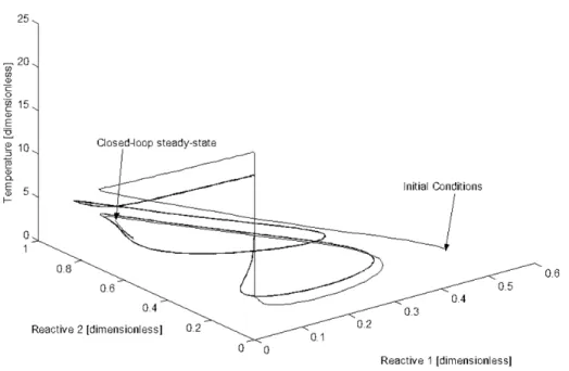
Figure 1 shows the closed-loop behavior in steady state of the corresponding space portrait; note the oscillatory behavior. All the variables in the figures in this work are dimensionless.

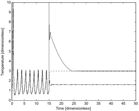
Closed loop performance of temperature trajectories show that the ideal I/O linearizing controller shows the best performance so that it cancels the nonlinearities, imposing a desired linear behavior, with a satisfactory performance. The proposed controller tries to compensate the nonlinear terms via the integral high-order sliding-mode contribution, besides it is able to reach the set point value required (Figure 2), exhibiting smaller oscillations around the regulated point (

3



sp



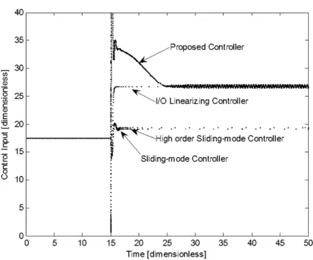
) than the other sliding-mode controllers. As predicted by the theoretical frame presented, sliding-mode and high order sliding-mode controllers can suppress nonlinear oscillations; however, both controllers exhibit a considerable off-set from the corresponding off-set point.

Figure 3 shows the corresponding estimation of the uncertainty. Another important difference is that effort performed by the manipulate variable (Figure

4) is very different for each controller. As it can be noticed, the I/O linearizing controller posseses the best performance, the sliding-mode controller exhibits the second smoothest behavior, followed by the high-order sliding-mode control, which exhibits more demanding effort at the start up of the regulation task. Finally, the proposed methodology shows the more demanding control action, where small oscillations are presented.

Comparing the performance and control effort, it is possible to note that the high-order sliding mode control is not very efficient because the regulated variable (temperature) exhibits the largest off-set, even when the effort is higher than in the case of the sliding-mode controller; nevertheless, the performance of the sliding-mode controller is not satisfactory because the set point are not reached. an be notice that the ideal I/O linearizing controller and the proposed controller are able to reach the corresponding set point, in some sense this is an advantage for the proposed methodology because in the case of this controller, the perfect knowledge of the model of the process is nor considere and its possible implementation looks more feasible than the ideal I/O controller.

Journal of Applied Research and Technology ₄₄₃

Figure 2. Closed-loop performance of the dimensionless temperature trajectories. ( ___ Proposed Controller; ideal I/O Linearizing

Controller; _ _ _ _ High-order Sliding-mode Controller; ... Sliding-mode controller).

Figure 3. Estimation of the uncertain term (dimensionless reaction heat).

0 5 10 15 20 25 30 35 40 45 50

0 1 2 3 4 5 6 7 8 9 10

Time [dimensionless]

T

em

pe

rat

u

re [

di

m

ens

io

nl

e

s

s

Temperature Control of Continuous Chemical Reactors Under Noisy Measurements and Model Uncertainties,Ricardo Aguilar López et al. / 428‐446 

Vol. 10, June 2012  444 

However, it is important to mention that the value of the control gains has to be chosen very carefully for the proposed methodology, such that with smaller values of control gains it is not possible to stabilize the oscillatory behavior of the chemical reactor, whereas for large values of these parameters, it is possible to lead to unacceptable control efforts or, even worse, to provoke additional closed-loop instabilities.

Besides, in order to measure the impact of the error, the “Integral Time-Weighted Squared Error” (ITSE) defined by (44) suggested by Ogunnaike and Ray [15] is employed. ITSE exhibits the advantage of heavy penalization of large errors at long time; therefore, is a good measure of resilience of the controller.







0 2

dt

t

ITSE



In order to compare the resilience of the controllers simulated, the ITSE was evaluated for the dynamic system under the influence of four controllers (Figure 5). As it is possible to note, and confirming the findings from Figure 2, the I/O linearizing and the proposed controller are the only two able to stabilize the system in the long time (

t



20

), whereas for sliding-mode and high order sliding- mode controllers this error increases in an unlimited way. This result is due to the ability of the controller proposed to eliminate offset, property that is not exhibited by the other controllers (Figure 2).

Figure 4. Practical effort of the controllers considered.