Quasi Sliding Mode Control of Generalized Lorenz Chaotic Systems

(1)

Abstract—This paper presents a systematic design procedure to stabilize generalized Lorenz chaotic systems based on sliding mode control. In contrast to the previous works of sliding mode control, the concept of quasi sliding mode control is firstly introduced such that continuous control input is obtained to avoid chattering phenomenon. Furthermore, under the proposed control law, the system states can be stabilized and driven into an arbitrary and predictable neighborhood of zero. This method can also be easily extended to a general class of chaotic systems.

Index Terms-- Quasi sliding mode control, chaos, generalized Lorenz chaotic systems, chattering phenomenon

I. INTRODUCTION

ver the last two decades, since the pioneering work of Ott, Grebogi and Yorke [1], chaos control has become one of interesting issues in nonlinear systems. A chaotic system is a very special nonlinear dynamical system and it possesses several properties such as the sensitivity to initial conditions, as well as an irregular, unpredictable behavior and thereby confines the precise operation of physical systems, such as mechanical systems, biological systems and power converters, etc. Therefore, various effective methods have been proposed over the past decades to achieve the control and stabilization of chaotic systems, such as optimal control [2], the sliding method control [3-8], state feedback control [9, 10] and the backstepping design technique [11, 12], etc.. In a robust control system, sliding mode control (SMC) is frequently adopted because SMC can offer many inherent advantages, such as fast response, good transient performance and insensitive to variation in plant parameters or external disturbances. However, in the conventional SMC systems [3-8], ideal sliding mode only exists with infinite frequency switching operation. From practical point of view, thus control input is impossible to implement and will cause the undesired chattering phenomenon.

Motivated by the aforesaid, this study aims to present a control scheme to suppress chaos for generalized Lorenz chaotic systems based on SMC. In contrast to the previous works of SMC, the concept of quasi sliding mode control (QSMC) is first introduced such that a continuous control input is obtained to avoid chattering phenomenon as frequently in the conventional sliding mode control systems. Furthermore, under the proposed control law, the system

The authors are with the Department of Computer and Communication, Shu-Te University, Kaohsiung 824, Taiwan, R.O.C.

* Corresponding author: J. J. Yan (E-mail: jjyan@ stu.edu.tw).

states can be stabilized and driven into an arbitrary and predictable neighborhood of zero. Finally, an illustrative example is presented to demonstrate the effectiveness of the proposed QSMC scheme.

II. SYSTEM DESCRIPTION AND PROBLEM FORMULATION In this section, we consider the chaos suppression of a generalized Lorenz chaotic system (GLCS) via a QSMC.

II.1 Generalized Lorenz chaotic systems

We consider the following GLCS:

[

]

T

[

]

T

x x x x

x x

t x t x t x k t

x

t x t x t x k t x k t

x

t x t x k t

x

30 20 10 3

2 1

2 1 3 3

3 1 2 1

2

1 2 1

) 0 ( ) 0 ( ) 0 (

) ( ) ( ) ( ) 87

1 3 8 ( ) (

) ( ) ( ) ( ) 1 ( ) ( ) 29 35 28 ( ) (

)] ( ) ( [ ) 29 25 10 ( ) (

= + −

− =

− −

+ −

=

− ⋅ + =

(1)

where

_[

_]

3

3 2

1() () ()

)

(t x t x t x t R

x = T∈ is state vector,

[

]

T

x x

x10 20 30 is the initial value vector, and k is the system

parameter with 0≤k<1. The dynamics of this system has been extensively studied in [13] for a space range of the amplitude of the term k and displays chaotic behavior for each

1

0≤k< . Figures 1(a)-(d) show the chaotic motion of system (1) for k=0.2 with initial condition of

[

]

T

[

]

T

x x

x₁₀ ₂₀ ₃₀ = 1　 1 0.5 . In the following, we will consider the chaos suppression of the GLCS and give an explicit and simple procedure to establish a QSMC to achieve the control goal.

II.2 Problem formulation

Consider the GLCS as shown in (1), to control the system effectively, we introduce a control input u to the differential

equation of state

2

x . By adding this input, the equation of the

controlled system can be expressed by

) ( ) ( ) ( ) 87

1 3 8 ( ) (

) ( ) ( ) ( ) 1 ( ) ( ) 29 35 28 ( ) (

)] ( ) ( [ ) 29 25 10 ( ) (

2 1 3 3

3 1 2 1

2

1 2 1

t x t x t x k t

x

u t x t x t x k t x k t

x

t x t x k t

x

+ −

− =

+ −

− + −

=

− ⋅ + =

(2)

The goal of this study is to design a QSMC such that the resulting state of system can be driven to predictable and desired bounds, i.e.

3 ,

2 ,

1 ,

lim

≤

=

∞

→

x

i i

i

t

γ

(3)

Quasi Sliding Mode Control of Generalized

Lorenz Chaotic Systems

Pei-Zhi Zhang-Jian, Chih-Yung Chen, Jun-Juh Yan*, Shih-Yao

Ying, Hun-Da Pei

O

Proceedings of the International MultiConference of Engineers and Computer Scientists 2011 Vol II, IMECS 2011, March 16 - 18, 2011, Hong Kong

ISBN: 978-988-19251-2-1

ISSN: 2078-0958 (Print); ISSN: 2078-0966 (Online)

(2)

where _≥₀

i

γ are predictable constants depending on the

parameter chosen in the QSMC, which will be stated later. In consequence, to achieve this control goal for the GLCS, there exist two major phases. First, it needs to select an appropriate switching surface for the system such that the quasi sliding motion on the manifold can result in

i i

t

lim

→∞

e

≤

γ

,

i

=

1 ,

2 ,

3

. Second, it needs to determine a

QSMC such that the existence of the quasi sliding manifold can be guaranteed.

III. SWITCHING SURFACE DESIGN AND DEFINITION OF QUASI SLIDING MANIFOLD

To complete the above two phases, a switching surface is defined as follows:

) ( ) ( )

(t x₂ t cx₁ t

s = + (4) where s∈R and c>−1 is a chosen constant. Therefore, the

following dynamics of x₁(t)in (2) can be obtained as ) ( ) 29 25 10 ( ) ( )

( ₁ ₁

1t x t k st

x =−λ + + (5)

where ₎₍₁ ₎

29 25 10 (

1= + k +c

λ .

Before continuing to discuss the response of state

1 x, we

give the definition of quasi sliding manifold as follows. Definition 1: The system is said to be in the quasi sliding manifold if there exists _>₀

Q

δ and t_Q>0 such that any solution _x₍_⋅₎ of controlled system (2) satisfies

Q

t

s() ≤δ , for all

Q

t

t≥ .

Solving the differential equation (5) for

1

x when t≥t_Q

results in

+ +

= − − t − −

t t Q t t Q Q d s e k t x e t

x ( )

1 ) (

1 ) ( )

29 25 10 ( ) ( )

( 1 1

τ τ

τ λ

λ ₍₆₎

As shown in Definition 1, when the system enters the quasi sliding manifold, one has

Q

t

s()≤δ for t≥tQ. Furthermore,

since c>−1 is determined to result in λ₁>0, the bound for state

1

x can be obtained as

1 ) ( 1 ) ( 1 ) ( ) ( 1 ) ( 1 1 1 1 1 1 1 1 1 ) 29 25 10 ( ) ( ) 29 25 10 ( ) ( ) ( ) 29 25 10 ( ) ( ) ( λ δ τ δ τ τ λ λ τ λ λ λ τ λ λ Q Q Q Q Q Q t t Q Q t t t t t Q Q t t t t t Q t t e k t x e d e e k t x e d s e k t x e t x − − − − − − − − − − − − + + = + + ≤ + + = (7)

Eqn. (7) with ₀

1>

λ ensures that

c k

t

x Q Q

t→∞ ≤ = +₂₉ ) =₁₊ 25 10 ( ) ( lim 1 1 1 δ λ δ

γ . (8)

Furthermore, by (4), the bound for x₂(t), t→∞ , can be also

obtained as Q t t t t c c t x c t s t cx t s t x δ γ ) 1 1 ( ) ( lim ) ( lim ) ( ) ( lim ) ( lim 2 1 1 2 + + = ≤ + ≤ − = ∞ → ∞ → ∞ → ∞

→ ₍₉₎

Meanwhile, after

i i

x ≤γ , i=1,2, solving the differential eqn. (2) for error state

x

₃ results in

) ( ) ( lim 87 1 3 8 2 1 3 3 k t x

t→∞ ≤ = ₊

γ γ

γ (10) Obviously, the bounds of _,_i₌₁_,₂_,₃

i

γ are relative to δQ.

Therefore, to control the system with a smaller value of

Q

δ is

important and the solution will be given in the following section.

IV. QSMC DESIGN FOR THE QUASI SLIDING MANIFOLD Having established an appropriate switching surface and estimating the bounds of the states of system, this section aims to design an QSMC to drive the dynamics (2) into the quasi sliding manifold,s(t)≤δ_Q. To ensure the occurrence of the quasi sliding manifold, the continuous QSMC is proposed as

δ η + − = s s w t

u() (11)

where w>1, δ>0and

) )( 29 25 10 ( ) 1 ( ) 29 35 28

( − k x₁+ k− x₂−x₁x₃+c + k x₂−x₁ =

η .

The proposed control scheme above will guarantee the quasi sliding mode motion for the system (2), and is proven in the following theorem.

Theorem 1: _{Consider the system (2), if this system is} controlled by u(t) in (11). Then the system trajectory converges to the quasi sliding manifold,

1 ) ( − = ≤ w w t s Q δ δ .

Proof of Theorem 1: Let the Lyapunov function of the

system be 2

2 1

s

V= , then taking the derivative of V and introducing (4) (11), one has

) ( )) )( 29 25 10 ( ) 1 ( ) 29 35 28 (( ) ( 2 1 2 3 1 2 1 1 2 δ δ η η δ η η + − − ≤ + − ≤ − + + + − − + − = + = = s s s w s s s w s x x k c u x x x k x k s x c x s s s V (12)

Since _δ

δ δ

≤ + s

s _{, we have}

) 1 ( ) 1 ( − − − ≤ − ≤ = w w s w w s s s V δ η ηδ

η (13)

ISBN: 978-988-19251-2-1

(3)

Since _w_>₁has been chosen in the controller (11), (13) implies that V<0 whenever

1 )

(

− = >

w w t

s Q

δ

δ . That is to say that s will converges to the region of

1 )

(

− = ≤

w w t

s Q

δ

δ .

Thus the proof is achieved completely.

Remark 1: Since the QSMC in (11) is continuous, chattering is eliminated.

Remark 2: In fact, δis a design parameter, in QSMC (11) therefore, one can select a sufficient small value of

δ

to make δ_Q as well as γi,i=1,2,3 arbitrarily bounded in the neighborhood of zero.

Remark 3: From the above analysis, a procedure for the robust control of chaos in the GLCS is proposed as follows. Step 1: Select c>−1 to ensure a stable quasi sliding manifold. Step 2: Obtain the switching function

s

from eq. (4) and select the control parameters in eqn. (11).

Step 3: Calculate the predictable error bounds _,_i₌₁_,₂_,₃

i

γ by

eqs.(8)-(11) to estimate the performance of control. Step4: QSMC from eqn. (11).

V. NUMERICAL EXAMPLE

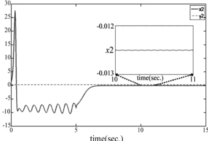
In this section, simulation results are presented to demonstrate and verify the effectiveness of the proposed QSMC scheme. The system parameter is chosen as k=0.2. The initial states are ₍₀₎ ₁

1 =

x , x₂(0)=1 , x3(0)=0.5 . According to step 1 in Remark 3, we select c=1>−1 to result in a bounded quasi sliding manifold. Therefore, the switching function

s

is

1 2

) (t x x

s = + (14)

and the QSMC can be obtained as δ

η

+ − =

s s w t

u() (15) withw=2>1, δ=0.05.

By eqns. (8)-(10), we can predict that ₍₎_≤ ₌₀_.₁

Q

t

s δ and

the states are bounded by ₀_.₀₂₅_, ₀_.₁₇₅

2

1 = γ =

γ , and

0016 . 0

3=

γ .The simulation results are shown in Figures 2-4. Figure 2 and Figure 3 present, respectively, the corresponding

)

(

t

s

and state responses. The continuous QSMC control is shown in Figure 4.For the first five seconds, the system is uncontrolled and the trajectories are chaotic and the QSMC (15) become active at t=5second and the system state can be bounded by _,_i₌₁_,₂_,₃

i

γ calculated above, as we predict. In particular, it is worthy of note that the chattering does not appear due to the continuous control input as shown in Figure 4.

VI. CONCLUSIONS

In this paper, a quasi sliding mode control scheme for generalized Lorenz chaotic systems is studied. The concept of

quasi sliding mode control has been introduced firstly to avoid chattering phenomenon as frequently in the conventional sliding mode control systems. Numerical simulations have verified the effectiveness of the proposed method.

REFERENCES

[1] E. Ott, C. Grebogi, J. A. Yorke, “Controlling chaos”, Phys Rev Lett, 1990, 64, pp. 1196-1199.

[2] M. T. Yassen, “The optimal control of Chen chaotic dynamical system”, Applied Mathematics and Computation, 2002, 131, pp. 171-180.

[3] H. Wang, Z. Z. Han, Q. Y. Xie, W. Zhang,“Sliding mode control for chaotic systems based on LMI”, Communications in Nonlinear Science and Numerical Simulation, Volume 14, Issue 4, April 2009, pp. 1410-1417.

[4] M. Roopaei, B. R. Sahraei, T. C. Lin,“Adaptive sliding mode control in a novel class of chaotic systems”,Communications in Nonlinear Science and Numerical Simulation, Volume 15, Issue 12, December 2010, pp. 4158-4170.

[5] K. Konishi, M. Hirai, H. Kokame, “Sliding mode control for a class of chaotic systems”, Physics LettersA, 1998, 245, pp. 511-517. [6] H. Guo, S. Lin, J. Liu, “A radial basis function sliding mode controller

for chaotic Lorenz system”, Physics Letters A, 2006, 351, pp. 257-261. [7] T. Y. Chiang, M. L. Hung, J. J. Yan, Y. S. Yang, J. F. Chang, “Sliding mode control for uncertain unified chaotic systems with input nonlinearity”, Chaos Soltions Fractals, 2007, 34, pp. 437-442. [8] S. K. Yang, C. L. Chen, H. T. Yau, “Control of chaos in Lorenz

system”, Chaos Soltions Fractals, 2002; 13, pp. 767-780.

[9] J. H. Park, D. H. J. Won, S. M. Lee, “_H_∞ synchronization of

time-delayed chaotic systems”, Applied Mathematics and Computation, 2008, 204, pp. 170-177.

[10] G. Chen, X. Dong, “On feedback control of chaotic dynamic systems”,

Int J Bifurcation Chaos, 1992, 2, pp. 407-411.

[11] T. Yang, L. O. Chua, “Impulsive stabilization for control and synchronization of chaotic systems: theory and application to secure communication”, IEEE Trans Circ Syst I, 1997, 44, pp. 976-988. [12] Y. Yu, S. Zhang, “Controlling uncertain Lu system using backstepping

design”, Chaos Soltions Fractals, 2003, 15, pp. 897-902.

[13] J. Lü , G. Chen, D. Z. Cheng, S. Celikovsky, “Bridge the gap between the Lorenz system and the Chen system”, Int J Bifurcat Chaos, Vol. 12, 2002, pp. 2917-2926.

ISBN: 978-988-19251-2-1

(4)

Fig. 3. (c). The state response of the controlled system.

Fig. 4. . The time response of continuous QSMC (15). Fig. 3. (b). The state response of the controlled system.

Fig. 3. (a). The state response of the controlled system. Fig. 2. The time response of switching function s(t)

Fig. 1. (a) Trajectories of GLCS (b) Trajectories projected on the

1 x

-2

x plane (c) Trajectories projected on the

1 x

-3

x plane (d)

Trajectories projected on the

2 x

-3 x plane.

ISBN: 978-988-19251-2-1