A method to derive the Site Atmospheric State Best Estimate (SASBE) of ozone profiles from radiosonde and passive microwave data

(1)

AMTD

8, 3399–3422, 2015

A method to derive the SASBE of ozone

profiles

E. Maillard Barras et al.

Title Page

Abstract Introduction

Conclusions References

Tables Figures

◭ ◮

Back Close

Full Screen / Esc

Printer-friendly Version Interactive Discussion

Discussion

P

a

per

|

Discussion

P

a

per

|

Discussion

P

a

per

|

Discussion

P

a

per

|

Atmos. Meas. Tech. Discuss., 8, 3399–3422, 2015 www.atmos-meas-tech-discuss.net/8/3399/2015/ doi:10.5194/amtd-8-3399-2015

This discussion paper is/has been under review for the journal Atmospheric Measurement Techniques (AMT). Please refer to the corresponding final paper in AMT if available.

A method to derive the Site Atmospheric

State Best Estimate (SASBE) of ozone

profiles from radiosonde and passive

microwave data

E. Maillard Barras, A. Haefele, R. Stübi, and D. Ruffieux

Federal Office of Meteorology and Climatology, MeteoSwiss, Switzerland

Received: 21 October 2014 – Accepted: 9 March 2015 – Published: 31 March 2015

Correspondence to: E. Maillard Barras (eliane.maillard@meteoswiss.ch)

(2)

AMTD

8, 3399–3422, 2015

profiles

Title Page

Tables Figures

◭ ◮

Back Close

Full Screen / Esc

Discussion

P

a

per

|

Discussion

P

a

per

|

Discussion

P

a

per

|

Discussion

P

a

per

|

Abstract

We present a method to derive the site atmospheric state best estimate (SASBE) of the ozone profile combining brightness temperature spectra around the 142 GHz ab-sorption line of ozone measured by the microwave radiometer SOMORA and ozone profiles measured by the radiosonde (RS). The SASBE ozone profile is obtained using

5

the radiosonde ozone profile as a priori information in an optimal estimation retrieval of the SOMORA radiometer. The resulting ozone profile ranges from ground up to 65 km altitude and makes optimal use of the available information at each altitude. The high vertical resolution of the radiosonde profile can be conserved and the uncertainty of the SASBE is well defined at each altitude.

10

A SASBE ozone profile dataset has been generated for Payerne, Switzerland, with a temporal resolution of 3 profiles a week for the time period ranging from 2011 to 2013. The relative difference of the SASBE ozone profiles to the AURA/MLS ozone profiles lies between −3 to 6 % over the vertical range of 20–65 km. Above 20 km,

the agreement between the SASBE and AURA/MLS ozone profiles is better than the

15

agreement between the operational SOMORA ozone data set and AURA/MLS. Below 20 km the SASBE ozone data are identical to the radiosonde measurements.

The same method has been applied to ECWMF-ERA interim ozone profiles and SOMORA data to generate a SASBE dataset with a time resolution of 4 profiles per day. These SASBE ozone profiles agree between−4 and +8 % with AURA/MLS. The

20

(3)

AMTD

8, 3399–3422, 2015

profiles

Title Page

Tables Figures

◭ ◮

Back Close

Full Screen / Esc

Discussion

P

a

per

|

Discussion

P

a

per

|

Discussion

P

a

per

|

Discussion

P

a

per

|

1 Introduction

Since the discovery of the ozone hole over Antarctica in 1983 (Chubachi, 1985; Far-man, 1985), the understanding of the mechanisms driving the variability of the strato-spheric ozone layer has been one of the major area of interest in atmostrato-spheric research. Dynamical (Miyazaki, 2005) and chemical (Revell, 2012) processes are considered

de-5

pending on time, location and altitude. The consideration of the entire vertical extent of the atmosphere and of the interaction between the different layers is of primary impor-tance in understanding the stratospheric ozone variability.

At many measurement sites, ozone measurements are performed by several in-struments, each of them covering a particular altitude range with different spatial or

10

temporal resolutions. Radiosondes are measuring ozone profiles from ground up to 30–35 km (Hassler, 2013), LIDAR measurements are performed during the night up to 50 km (Pelon, 1986), and microwave radiometers (MWR) measure ozone profiles from the lower stratosphere up to the lower mesosphere with a high temporal resolution. Satellites regularly overpass the ground measurement sites and measure ozone

pro-15

files from 10 to 70 km (Hassler, 2013). Dobson and Brewer spectrometers measure the ozone total column up to more than 100 times a day depending on the meteorological situation (Scarnato, 2010). Hence, in order to obtain a continuous ozone profile rang-ing from the ground up to the mesosphere, the different observation methods need to be combined. This is one of the recommendations for an optimal observation strategy

20

by GRUAN (GCOS Reference Upper Air Network) for atmospheric parameters (WMO, 2013).

Various methods for the combination of ozone profiles have been reported in the literature in the perspective of a temporal (DeLand, 2012) or spatial (Bodeker, 2012) merging of datasets. In particular, when complementary but overlapping vertical

pro-25

(4)

AMTD

8, 3399–3422, 2015

profiles

Title Page

Tables Figures

◭ ◮

Back Close

Full Screen / Esc

Discussion

P

a

per

|

Discussion

P

a

per

|

Discussion

P

a

per

|

Discussion

P

a

per

|

Godson equation (Goody, 1989) which conserves the column density in the profile to be downscaled. If an averaging kernel is provided along with the low resolution data, the high resolution data can be convoluted with this averaging kernel (Tsou, 1995; Calisesi, 2005). A third method to downscale the high resolution data consists of ap-plying a Gaussian filter centered around the levels of the coarse grid on the high

reso-5

lution data as it has been done for the “Binary Database of Profiles” of Hassler et al. to combine ozone sonde and satellite vertical profiles (Hassler, 2008). Finally, Livesey et al. (2011) suggest to compute the inverse of matrix A which describes the linear interpolation from the coarse to the high resolution grid and to applyA−1 to the high resolution data. For instruments with similar vertical resolution or once the vertical

res-10

olution has been adjusted using one of the methods explained above, a linear interpo-lation in the logarithm-pressure vertical coordinate can be used in the overlap region to merge the profiles (Sofieva, 2014). These merging methods do not preserve the origi-nal vertical resolution of the profiles involved in the combination, the vertical resolution of the combined profiles being either one of the original resolutions or a new

com-15

mon resolution. Alternatively, data can also be combined on the level of the raw data. Timofeyev et al. (2013) have proposed to combine Fourier transform infrared radiome-ter (FTIR) and MWR spectral data by retrieving a single ozone profile simultaneously from both spectral measurements or by sequential retrievals using the profile and the covariance matrix of the first retrieval step (FTIR) as an a priori information for the

sec-20

ond retrieval step (MWR). This method allows to choose the vertical grid freely or to optimize it given the degrees of freedom of the retrieval.

At the measurement site of MeteoSwiss in Payerne, ozone measurements are per-formed by radiosondes (Stübi, 2008) since 1968 and by microwave radiometry since 2000 (Calisesi, 2000). Here, we propose to combine the simultaneous radiosonde and

25

(5)

reso-AMTD

8, 3399–3422, 2015

profiles

Title Page

Tables Figures

◭ ◮

Back Close

Full Screen / Esc

Discussion

P

a

per

|

Discussion

P

a

per

|

Discussion

P

a

per

|

Discussion

P

a

per

|

lutions of the radiosonde ozone profiles and of the microwave ozone profiles are pre-served in the SASBE ozone profiles and that the uncertainty is well characterized at each altitude level.

The paper is organized as follows: Sect. 2 deals with the description of the instru-ments, and of the measured and simulated datasets used in the study. A detailed

de-5

scription of the merging method and a characterization of the retrieved profiles are given in Sects. 3 and 4. In Sect. 5, the SASBE ozone profiles are compared to simul-taneous satellite ozone profiles measured by AURA/MLS. The agreement of SASBE ozone profiles, using either RS or ECMWF ozone profiles, and of SOMORA ozone profiles with MLS ozone profile are finally discussed.

10

2 Instruments and models

2.1 Stratospheric Ozone Monitoring Radiometer SOMORA

Developed in 2000 by the University of Bern (Calisesi, 2000), the SOMORA is a to-tal power microwave radiometer measuring the thermal emission line of ozone at 142.175 GHz. The electromagnetic radiation is measured under an antenna elevation

15

angle of 39◦and the brightness temperatures range from 80 to 260 K. The SOMORA is calibrated using a hot load heated and stabilized at 300 K and a cold load at 77 K cooled with liquid nitrogen. A rotating planar mirror is used as a switch between the radiation sources. A Martin–Puplett interferometer (sideband filter) picks out the frequency band around 142 GHz. Outgoing from the front-end part (quasi optics), the signal is

ampli-20

fied and down-converted in frequency to 7.1 GHz by means of a constant-frequency signal (mixer). The signal is further down-converted in two steps (intermediate step at 1.5 GHz/1 GHz) to the baseband (0–1 GHz). The spectral distribution, i.e. voltage as function of channel or frequency is measured since 10/2010 by an Acquiris Fast– Fourier–Transform spectrometer (FFTS) with 16 384 channels distributed over 1 GHz

25

(6)

spec-AMTD

8, 3399–3422, 2015

profiles

Title Page

Tables Figures

◭ ◮

Back Close

Full Screen / Esc

Discussion

P

a

per

|

Discussion

P

a

per

|

Discussion

P

a

per

|

Discussion

P

a

per

|

tral detection (Calisesi, 2000). This study has been performed using spectra measured after the FFTS upgrade of the instrument.

After 30 min integration time, an ozone volume mixing ratio (VMR) profile is retrieved by optimal estimation using ARTS/Qpack, which is a general environment for the ra-diative transfer simulation (forward model) (Buehler, 2005) and the optimal estimation

5

method (OEM) profile retrieval of Rodgers (Eriksson, 2005). The vertical resolution of the ozone profiles is 8–10 km from 20 to 40 km, increasing to 15–20 km at 60 km.

The measured spectrumyis a functionF(x,b) of the vertical distribution of ozonex

and forward model parametersb(atmospheric temperature, spectroscopic data, mea-surement geometry, . . .). The OEM solution ˆx to the inverse problem minimizes the

10

cost functionχ2derived from the Bayesian theory:

χ2=[y−F(x,b)]TS−1

y [y−F(x,b)]+

x−x_aTS−1 a

x−x_a (1)

wherey is the measured spectrum, F(x,b) the calculated spectrum corresponding to the ozone profile x and model parameters b, x the true ozone profile, S_y the error covariance matrix of the measured spectrum,x_athe a priori ozone profile andS_a the

15

error covariance matrix of the a priori ozone profile.

The optimal estimation method takes into account the uncertainties of the measured spectrum specified inS_y and uses a priori information specified by x_a andS_a to con-strain the solution ˆxto statistically probable profiles. In the operational data processing of SOMORA two different a priori ozone profiles are used, one for summer and one

20

for winter. These a priori profiles are derived from the two standard model ozone pro-files described in (Keating, 1990) combining 5 satellite ozone data sets (among them SAGE and SBUV). The diagonal elements of the a priori covariance matrix are given by the variance of a climatology of Payerne radiosondes below 25 km and of a clima-tology of MWR ozone profiles above 25 km (climaclima-tology of the microwave radiometer

25

(7)

AMTD

8, 3399–3422, 2015

profiles

Title Page

Tables Figures

◭ ◮

Back Close

Full Screen / Esc

Discussion

P

a

per

|

Discussion

P

a

per

|

Discussion

P

a

per

|

Discussion

P

a

per

|

averaging kernel (AVK) matrix describing the changes in the retrieved profile,∂xˆ, as a function of changes in the true profile,∂x:

AVK=∂xˆ

∂y ∂y

∂x (2)

The AVK shows the sensitivity of the retrieved profile to the changes of the true profile. For an ideal observing system, the AVK is equal to the unity matrix. For a real

in-5

strument, the width of the AVKs is a measure of the resolution of the system (Rodgers, 1990). The area of the AVKs is indicating the measurement contribution to the retrieved profile. The total uncertainty of the retrieved profile consists of the observation and the smoothing error. The smoothing error is the error contribution due to the smoothing of the true state by the AVK. The observation error is to the greatest extent due to

10

the thermal noise in the spectral data, and to minor extent due to errors in the Tem-perature profile and the antenna elevation angle error, which are part of the forward model parameters b. The observation error is less than 3 % between 20 and 40 km, but increases to 7 % in the upper stratosphere.

The total error (sum of observation error and smoothing error) is less than 10 %

15

between 20 and 40 km, 15 % at 50 km, and greater than 25 % below 15 and above 60 km.

SOMORA has been extensively used in comparisons with AURA/MLS and SAGE (Hocke, 2007), ENVISAT (Hocke, 2006), LIDAR (Calisesi, 2003a), and radiosonde (Calisesi, 2003b). SOMORA belongs to the Network for the Detection of Atmospheric

20

Composition Change (NDACC).

2.2 Ozone radiosonde

Ozone sondes are launched from Payerne since 1968 (Stübi, 2008). The ozone sonde consists of an electrochemical cell where the reaction of ozone with potassium iodide in aqueous solution is used to measure continuously the ozone concentration. An

electri-25

(8)

AMTD

8, 3399–3422, 2015

profiles

Title Page

Tables Figures

◭ ◮

Back Close

Full Screen / Esc

Discussion

P

a

per

|

Discussion

P

a

per

|

Discussion

P

a

per

|

Discussion

P

a

per

|

The ozone concentration is determined from the electric current measurement con-sidering the airflow rate, the air pressure, and the pump temperature. Since Septem-ber 2002, the electrochemical concentration cell (ECC) with 0.5 % KI concentration is the operational ozone sensor for Payerne.

Ozone is measured in the altitude range of 0 to 30–35 km every Monday, Wednesday

5

and Friday. The vertical resolution is 150 m and the uncertainty of the ozone measure-ment is of the order of 5–10 % depending on the altitude (Stübi, 2008; Dabberdt, 2003). Payerne ozone sonde profiles are submitted to WOUDC and NDACC on an oper-ational basis, and are extensively used in satellite validation programs (Meijer, 2004) and ozone assessments (Douglass, 2011).

10

2.3 ECMWF ERA-Interim model

Six hourly ozone profiles from ERA-Interim are used in this study. The ERA-Interim reanalysis is produced with a sequential data assimilation scheme described in Dee et al. (2011). Ozone is analysed simultaneously with the other model state variables in the 4D-Var analysis. At a given point of the atmosphere, the continuity equation

15

for ozone is given as a linear relaxation towards a photochemical equilibrium for the ozone mixing ratio, the temperature, and the ozone column. The photochemical loss term is a function of the equivalent chlorine content for the actual year. A large va-riety of satellite observations are assimilated: MIPAS, SCIAMACHY, TOMS, GOME, MLS, OMI (Dragani, 2010). The ozone sonde data are not assimilated in ERA-Interim

20

but comparisons are described by Dragani et al. (2010). At midlatitudes in the North-ern Hemisphere, the agreement between sondes and ERA-Interim is within 5 % in the troposphere. The seasonal variability is well captured for total ozone and temporal oc-currence with an agreement of 10 % in the stratosphere. However, the ozone peak is underestimated by ERA-Interim in summer periods, with relative biases of about 20 %

25

(9)

AMTD

8, 3399–3422, 2015

profiles

Title Page

Tables Figures

◭ ◮

Back Close

Full Screen / Esc

Discussion

P

a

per

|

Discussion

P

a

per

|

Discussion

P

a

per

|

Discussion

P

a

per

|

3 Method

The SASBE of ozone is computed using the radiosonde measurement as a priori infor-mation in the optimal estiinfor-mation retrieval of SOMORA, which is described in Sect. 2.1. The retrieval grid, i.e. the grid of the resulting SASBE ozone profile, is equal to the standard grid of the radiosonde profile up to 25 km with a grid spacing of 500 m. Above

5

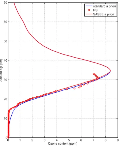
25 km, the standard SOMORA retrieval grid is used with a grid spacing of 2500 m. The a priori profile is identical to the radiosonde ozone measurement below 23 km. Above 35 km the standard SOMORA a priori profile is chosen as explained in Sect. 2.1. In order to avoid discontinuities in the a priori profilex_a, a weighting functionf increasing linearly from 0 to 1 between 23 and 35 km is applied to the standard a priori x_SOM,

10

which has been interpolated to the high resolution grid, and the radiosonde profilex_RS

(see Fig. 1):

x_a₌fx_SOM₊(1−f)x_RS (3)

Since the a priori profile below 23 km comes from the radiosonde measurement, the diagonal elements of the a priori covariance matrixS_aare populated with the square of

15

measurement uncertainties of the radiosonde measurement as specified in Sect. 2.2. Above 23 km the diagonal elements are identical to the a priori covariance matrix of the standard SOMORA retrieval as described in Sect. 2.1.

The off-diagonal elements are parameterized with an exponentially decaying corre-lation function using a correcorre-lation length of 150 m below 25 km which corresponds to

20

the vertical resolution of the RS ozone profile.

The SASBE retrieval provides an ozone profile from the surface up to 65 km that is based on measurements. Whether the information comes from the radiosonde or the microwave measurement is determined by the confidence in the measurement and the a priori profile, i.e. bySy andSa. Visual inspection of Fig. 2b shows that the information

25

(10)

AMTD

8, 3399–3422, 2015

profiles

Title Page

Tables Figures

◭ ◮

Back Close

Full Screen / Esc

Discussion

P

a

per

|

Discussion

P

a

per

|

Discussion

P

a

per

|

Discussion

P

a

per

|

A SASBE is also generated using ERA interim. In that case the ECMWF-ERA interim ozone profiles are processed in the same way as the radiosonde but we refer to “SASBE using ECMWF”. The diagonal elements of the a priori covariance matrix below 23 km are the square of the model uncertainties estimated through the comparison of ECMWF-ERA interim data with ECC radiosonde profiles (see Sect. 2.3).

5

The off-diagonal elements are kept the same as in the standard SOMORA retrieval.

4 Characterization of the SASBE ozone profile

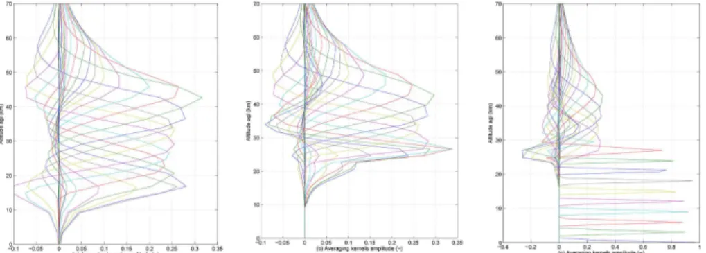
The SASBE ozone profile is characterized by the AVK functions and by the uncertain-ties shown in Figs. 2 and 3, respectively.

The AVKs are plotted in Fig. 2a for the SOMORA retrieval and in Fig. 2b and c

10

for the SASBE retrieval. In the case of SOMORA retrieval, the AVKs vanish below approximately 15 km indicating that the measurement does not contain any information about ozone below this altitude. In the case of the SASBE retrieval, it can be seen that the AVKs tend to zero already at 25 km which is due to the fact that a much higher confidence in the a priori profile has been specified (Fig. 2b). Similar smoothing of the

15

true state above 30 km are shown for both retrievals by the width of the AVK functions. However, to give a complete characterization of the SASBE retrieval with the AVKs, the a priori profile below 25 km must be considered as a measurement. Therefore any variation in the true atmosphere is captured in the a priori profile and seen in the SASBE profile. The completeAVK as shown in Fig. 2c has been calculated with

20

a perturbation approach: a true ozone profile has been assumed from which both the radiosonde and the microwave radiometer measurements have been calculated. The calculated measurements have been processed by the SASBE algorithm providing the retrieval for the unperturbed profile. Then the true profile has been perturbed with 1 ppm additional ozone at layeri. The measurements have been simulated from the perturbed

25

(11)

AMTD

8, 3399–3422, 2015

profiles

Title Page

Tables Figures

◭ ◮

Back Close

Full Screen / Esc

Discussion

P

a

per

|

Discussion

P

a

per

|

Discussion

P

a

per

|

Discussion

P

a

per

|

is taken from the radiosonde measurement in the SASBE algorithm. The difference between the retrieval of the perturbed state and the unperturbed state divided by the norm of the perturbation yields the averaging kernel function for leveli. The procedure is repeated for all levels to form the averaging kernel matrix.

The complete AVK show clearly the very high sensitivity and vertical resolution in

5

the altitude range where the in situ radiosonde measurement is available, similar to an ideal measurement system.

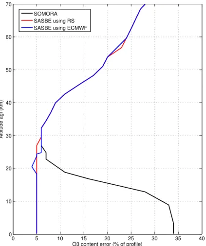
The uncertainties of the SOMORA and the SASBE retrievals are shown in Fig. 3. It is in the nature of the optimal estimation method that the error become equal to the a priori errors in the altitude ranges where the measurement contribution is small.

10

Therefore, the errors increase below 20 and above 60 km to the a priori uncertainties. In the case of the SOMORA retrieval, the error below 20 km increases to 35 % due to the large a priori uncertainty while the error of the SASBE retrieval remains small at 6 % below 20 km reflecting the low a priori error. The error is in both cases around 10 % at 40 km.

15

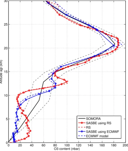
An example of a SOMORA and SASBE retrieval is shown in Fig. 4. The SASBE shows a very good correspondence to the RS ozone profile in dashed red. A very good correspondence is also shown between the ECMWF profile in dashed blue and the SASBE using ECMWF ozone profile in solid blue.

The sampling rate of the SASBE ozone profile dataset is 3 times a week for the

com-20

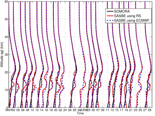
bination of RS and MWR data and 4 times a day for the combination of ECMWF model and MWR ozone profiles. The ozone profile time series over Payerne are available in a special dataset (shown in nbar for 2 monthes in Fig. 5) composed by MWR ozone profiles in the range of 20 to 65 km each 30 min (in black), SASBE ozone profiles 3 times a week (in red) in the range of ground up to 65 km and SASBE using ECMWF 4

25

(12)

AMTD

8, 3399–3422, 2015

profiles

Title Page

Tables Figures

◭ ◮

Back Close

Full Screen / Esc

Discussion

P

a

per

|

Discussion

P

a

per

|

Discussion

P

a

per

|

Discussion

P

a

per

|

5 Validation by comparison to AURA/MLS and Payerne RS

Payerne SASBE and SASBE using ECMWF ozone profiles from 2011 to 2013 have been compared to simultaneous MLS and radiosonde measurements. The following time and spatial coincidence conditions have been chosen in order to ensure reason-able overpass statistics while avoiding sampling issues. The time coincidence condition

5

is±4 h and the spatial coincidence condition is ±2.5◦ in latitude and±5◦ in longitude.

Payerne RS time coincidence condition is±1 h.

Above 25 km, MLS ozone profile have been downscaled to the vertical resolution of SOMORA resp. SASBE using AVK smoothing (Tsou, 1995) as follows:

Xsat, low=Xapriori, SOMORA resp. SASBE+ASOMORA resp. SASBE

10

(Xsat, high−Xapriori, SOMORA resp. SASBE) (4)

XRS, low=Xapriori, SOMORA resp. SASBE+ASOMORA resp. SASBE

(X_{RS, high}−Xapriori, SOMORA resp. SASBE) (5)

X_{apriori, SOMORA resp. SASBE} is the a priori profile of the standard SOMORA and the SASBE retrieval, respectively, and ASOMORA resp. SASBE is the averaging kernel matrix

15

of the corresponding retrieval. Xsat, low resp. XRS, low is the downscaled profile of the

satellite and RS measurement, respectively, adjusted to the vertical resolution of the SASBE.

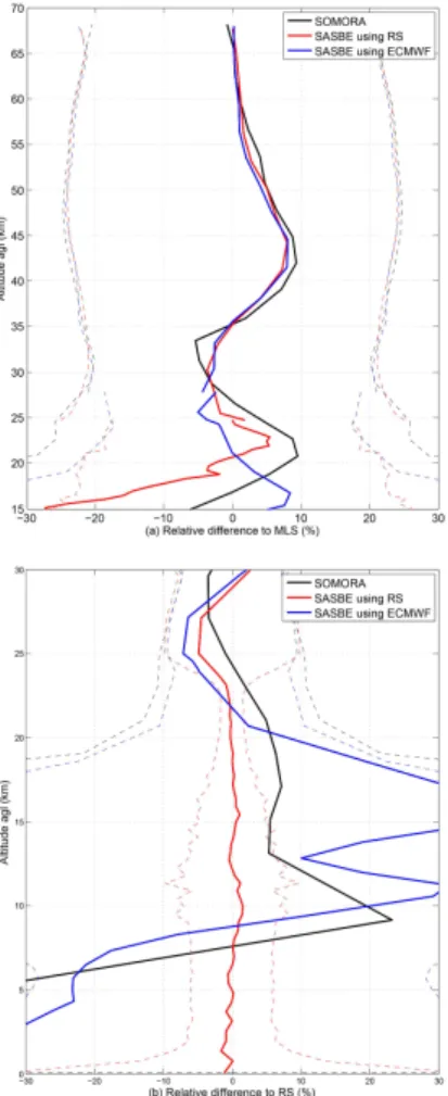
The arithmetic averages of the relative differences of SOMORA resp. SASBE to MLS and RS are shown in Fig. 6a and b. The relative difference between the RS ozone

20

profiles and the SASBE (using RS) profiles is smaller than 6 % below 20 km with no systematic bias as expected. The SASBE using ECMWF profiles show a difference with RS profiles as high as 35 % at 15 km. This is in accordance with the relative dif-ference between ECWMF ERA Interim and RS ozone profiles as reported in Dragani et al. (2010).

25

(13)

pro-AMTD

8, 3399–3422, 2015

profiles

Title Page

Tables Figures

◭ ◮

Back Close

Full Screen / Esc

Discussion

P

a

per

|

Discussion

P

a

per

|

Discussion

P

a

per

|

Discussion

P

a

per

|

files agree within 6 % with MLS/AURA satellite ozone profiles which is a slight improve-ment compared to standard SOMORA ozone profiles. This improveimprove-ment is related to the fact that smaller a priori errors below 25 km are lowering the cost corresponding to the state vector and therefore influencing the retrieval stability well over the RS altitude range. The SASBE using ECMWF agrees within 8 % with MLS which is also slightly

5

better than the standard SOMORA retrieval. The SD of the relative differences is be-tween 15 and 20 % for standard SOMORA and SASBE. Comparisons below 25 km show that the SASBE is unbiased compared to the radiosonde and that the proposed method does not have any degrading effect on the lower part of the profile.

6 Conclusions

10

Ozone profiles measured simultaneously by microwave radiometry and radio sounding over Payerne have been combined in one single ozone profile conserving maximum vertical resolution of both measurements. In the presented approach, the radiosonde ozone profile has been used as the a priori information in the optimal estimation re-trieval of the SOMORA radiometer. The a priori covariance matrix has been adjusted

15

representing the measurement uncertainty of the radiosonde in the corresponding al-titude range, i.e. below 25 km. The resulting profile, called SASBE, makes an optimal use of the available information at each altitude of the range and is fully characterized in terms of uncertainty and vertical resolution. An extendedAVK has been calculated representing the total measurement process including the radiosonde. It reveals that

20

the SASBE is sensitive to atmospheric variations at altitudes from the ground up to approximately 65 km. The uncertainty of the SASBE is 5 % up to 30 km and increases nearly linearly above to 25 % at 65 km.

A new 3 year dataset of SASBE and SASBE using ECMWF ozone profiles has been generated with a temporal sampling of 3/week and 4/day, respectively. The vertical

25

(14)

AMTD

8, 3399–3422, 2015

profiles

Title Page

Tables Figures

◭ ◮

Back Close

Full Screen / Esc

Discussion

P

a

per

|

Discussion

P

a

per

|

Discussion

P

a

per

|

Discussion

P

a

per

|

SASBE ozone profiles compared to a range from 20 to 65 km in the case of the stan-dard SOMORA retrieval.

The SASBE and SASBE using ECMWF data sets have been validated against Aura/MLS ozone profiles. The comparison revealed an improved agreement with Aura/MLS in the altitude range from 25 to 65 km for both data sets compared to the

5

standard SOMORA retrieval. This improvement is clearly attributed to the better a pri-ori information below 25 km and is remarkable since the improvement is seen at higher altitudes.

The SASBE dataset over Payerne is available for validation of satellite and other remote sensing instrument ranging from ground to 65 km height with a temporal

reso-10

lution of 3 times a week for SASBE (using RS) and of 6 h for SASBE using ECMWF. The presented approach to combine measurements is equivalent to 1-D variational data assimilation. It can be considered as a general framework for data fusion and provides a single atmospheric state that is consistent with an arbitrary number of ob-servations allowing for a detailed characterization of the result in terms of uncertainty

15

and resolution.

Acknowledgements. This work has been funded by MeteoSwiss within the Swiss Global

Atmo-spheric Watch (GAW) program of the World Meteorological Organization.

References

Bodeker, G. E., Hassler, B., Young, P. J., and Portmann, R. W.: A vertically resolved, global,

20

gap-free ozone database for assessing or constraining global climate model simulations, Earth Syst. Sci. Data, 5, 31–43, doi:10.5194/essd-5-31-2013, 2013.

Buehler, S. A., Eriksson, P., Kuhn, T., von Engeln, A., and Verdes, C.: ARTS, the Atmospheric Radiative Transfer Simulator, J. Quant. Spectrosc. Ra., 91, 65–93, doi:10.1016/j.jqsrt.2004.05.051, 2005.

25

(15)

Philosophisch-AMTD

8, 3399–3422, 2015

profiles

Title Page

Tables Figures

◭ ◮

Back Close

Full Screen / Esc

Discussion

P

a

per

|

Discussion

P

a

per

|

Discussion

P

a

per

|

Discussion

P

a

per

|

Naturwissenschaftliche Fakultät, Universität Bern, Bern, Switzerland, 77 pp., available at: http://www.iap.unibe.ch/publications (last access: 20 March 2015), 2000.

Calisesi, Y., Ruffieux, D., Kämpfer N., and Viatte, P.: The Stratospheric Ozone Monitoring Ra-diometer SOMORA: first validation results, in: Proceedings of the Sixth European Sympo-sium on Stratospheric Ozone, Göteborg, Sweden, 2–6 September 2002, 92–95, 2003a.

5

Calisesi, Y., Stuebi, R., Kämpfer, N., and Viatte, P.: Investigation of systematic uncertainties in Brewer–Mast ozone soundings using observations from a ground-based microwave ra-diometer, J. Atmos. Ocean. Tech., 20, 1543–1551, 2003b.

Calisesi, Y., Soebijanta, V. T., and van Oss, R. O.: Regridding of remote soundings: for-mulation and application to ozone profile comparison, J. Geophys. Res., 110, D23306,

10

doi:10.1029/2005JD006122, 2005.

Chubachi, S.: A special ozone observation at Syowa station, Antarctica from February 1982 to January 1983, in: Atmospheric Ozone, edited by: Zerefos, C. and Ghazi, A., Springer Netherlands, 6099, 285–289, doi:10.1007/978-94-009-5313-0_58, 1985.

Dabberdt, W. F. and Shellhorn, R.: Radiosondes, edited by: Shankar, M., available at: http:

15

//radiosondemuseum.org/wp-content/uploads/2012/10/RadiosondeArticle.pdf (last access: 20 March 2015), 2003.

Dee, D. P., Uppala, S. M., Simmons, A. J., Berrisford, P., Poli, P., Kobayashi, S., Andrae, U., Balmaseda, M. A., Balsamo, G., Bauer, P., Bechtold, P., Beljaars, A. C. M., van de Berg, L., Bidlot, J., Bormann, N., Delsol, C., Dragani, R., Fuentes, M., Geer, A. J.,

Haim-20

berger, L., Healy, S. B., Hersbach, H., Holm, E. V., Isaksen, L., Kallberg, P., Köhler, M., Matricardi, M., McNally, A. P., Monge-Sanz, B. M., Morcrette, J., Park, B., Peubey, C., de Rosnay, P., Tavolato, C., Thépaut, J., Vitart, F.: The ERA-Interim reanalysis: configuration and performance of the data assimilation system, Q. J. Roy. Meteor. Soc., 137, 553–597, doi:10.1002/qj.828, 2011.

25

DeLand, M. T., Taylor, S. L., Huang, L. K., and Fisher, B. L.: Calibration of the SBUV version 8.6 ozone data product, Atmos. Meas. Tech., 5, 2951–2967, doi:10.5194/amt-5-2951-2012, 2012.

Douglass, A., Fioletov, V., (Coordinating Lead Authors), Godin-Beekmann, S., Müller, R., Sto-larski, R. S., and Webb, A.: Stratospheric ozone and surface ultraviolet radiation, in: Scientific

30

(16)

AMTD

8, 3399–3422, 2015

profiles

Title Page

Tables Figures

◭ ◮

Back Close

Full Screen / Esc

Discussion

P

a

per

|

Discussion

P

a

per

|

Discussion

P

a

per

|

Discussion

P

a

per

|

Dragani, R.: On the quality of the ERA-Interim ozone reanalyses, Part I: Comparisons with in situ measurements, ERA Report Series, No. 2, ECMWF, Reading, UK, 2010.

Eriksson, P., Jimenez, C., and Buehler, S. A.: Qpack, a general tool for instrument simula-tion and retrieval work, J. Quant. Spectrosc. Ra., 91, 47–64, doi:10.1016/j.jqsrt.2004.05.050, 2005.

5

Farman, J. C., Gardiner, B. G., and Shanklin, J. D.: Large losses of total ozone in Antarctica reveal seasonal ClO_x/NO_xinteraction, Nature, 315, 207–210, doi:10.1038/315207a0, 1985. Goody, R. M. and Jung, Y. L.: Atmospheric Radiation: Theoretical Basis, 2nd edn., Oxford Univ.

Press, New York, 519 pp., 1989.

Hassler, B., Bodeker, G. E., and Dameris, M.: Technical Note: A new global database of trace

10

gases and aerosols from multiple sources of high vertical resolution measurements, Atmos. Chem. Phys., 8, 5403–5421, doi:10.5194/acp-8-5403-2008, 2008.

Hassler, B., Petropavlovskikh, I., Staehelin, J., August, T., Bhartia, P. K., Clerbaux, C., De-genstein, D., Mazière, M. De, Dinelli, B. M., Dudhia, A., Dufour, G., Frith, S. M., Froide-vaux, L., Godin-Beekmann, S., Granville, J., Harris, N. R. P., Hoppel, K., Hubert, D.,

Ka-15

sai, Y., Kurylo, M. J., Kyrölä, E., Lambert, J.-C., Levelt, P. F., McElroy, C. T., McPeters, R. D., Munro, R., Nakajima, H., Parrish, A., Raspollini, P., Remsberg, E. E., Rosenlof, K. H., Rozanov, A., Sano, T., Sasano, Y., Shiotani, M., Smit, H. G. J., Stiller, G., Tamminen, J., Tarasick, D. W., Urban, J., van der A, R. J., Veefkind, J. P., Vigouroux, C., von Clarmann, T., von Savigny, C., Walker, K. A., Weber, M., Wild, J., and Zawodny, J. M.: Past changes in the

20

vertical distribution of ozone – Part 1: Measurement techniques, uncertainties and availabil-ity, Atmos. Meas. Tech., 7, 1395–1427, doi:10.5194/amt-7-1395-2014, 2014.

Hocke, K., Haefele, A., Le Drian, C., Kaempfer, N., Ruffieux, D., von Clarmann, T., Milz, M., Steck, T., Froidevaux, L., Pumphrey, H. C., Jimenez, C., Walker, K. A., Bernath, P., Tim-ofeyev, Y. M., and Polyakov, A. V.: Cross-validation of recent satellite and ground-based

25

measurements of ozone and water vapor in the middle atmosphere, in: ESA Atmospheric Science Conference 2006, Frascati, Italy, 8–12 May 2006.

Hocke, K., Kämpfer, N., Ru_ffieux, D., Froidevaux, L., Parrish, A., Boyd, I., von Clarmann, T., Steck, T., Timofeyev, Y. M., Polyakov, A. V., and Kyrölä, E.: Comparison and synergy of strato-spheric ozone measurements by satellite limb sounders and the ground-based microwave

30

(17)

AMTD

8, 3399–3422, 2015

profiles

Title Page

Tables Figures

◭ ◮

Back Close

Full Screen / Esc

Discussion

P

a

per

|

Discussion

P

a

per

|

Discussion

P

a

per

|

Discussion

P

a

per

|

Keating, G. M., Pitts, M. C., and Young, D. F.: Ozone reference models for the middle atmo-sphere, Adv. Space Res., 10, 12-317–12-355, 1990.

Livesey, N. J., Read, W. G., Froidevaux, L., Lambert, A., Manney, G. L., Pumphrey, H. C., San-tee, M. L., Schwartz, M. J., Wang, S., Cofeld, R. E., Cuddy, D. T., Fuller, R. A., Jarnot, R. F., Jiang, J. H., Knosp, B. W., Stek, P. C., Wagner, P. A., and Wu, D. L.: Version 3.3 Level 2

5

data quality and description document, California Institute of Technology, Pasadena, Califor-nia, available at: http://mls.jpl.nasa.gov/data/v3-3_data_quality_document.pdf (last access: 20 March 2015), 2011.

Meijer, Y. J., Swart, D. P. J., Koelemeijer, R., Allaart, M., Andersen, S., Bodeker, G., Boyd I., Braathen, G., Calisesi, Y., Claude, H., Dorokhov, V., von der Gathen, P., Gil, M.,

Godin-10

Beekmann, S., Goutail, F., Hansen, G., Karpetchko, A., Keckhut, P., Kelder, H., Kois, B., Koopman, R., Lambert, J., Leblanc, T., McDermid, I. S., Pal, S., Raffalski, U., Schets, H., Stubi, R., Suortti, T., Visconti, G., and Yela, M.: Pole-to-pole validation of ENVISAT GOMOS ozone profiles using data from ground-based and balloon-sonde measurements, J. Geophys. Res., 109, 2156–2202, doi:10.1029/2004JD004834, 2004.

15

Miyazaki, K., Iwasaki, T., Shibata, K., and Deushi, M.: Roles of transport in the seasonal varia-tion of the total ozone amount, J. Geophys. Res., 110, D18309, doi:10.1029/2005JD005900, 2005.

Pelon, J., Godin, S., and Mégie, G.: Upper stratospheric (30–50 km) lidar ob-servations of the ozone vertical distribution, J. Geophys. Res., 91, 8667–8671,

20

doi:10.1029/JD091iD08p08667, 1986.

Revell, L. E., Bodeker, G. E., Huck, P. E., Williamson, B. E., and Rozanov, E.: The sensitivity of stratospheric ozone changes through the 21st century to N₂O and CH₄, Atmos. Chem. Phys., 12, 11309–11317, doi:10.5194/acp-12-11309-2012, 2012.

Rodgers, D. C.: Characterisation and error analysis of profiles retrieved from remote sensing

25

measurements, J. Geophys. Res., 95, 5587–5595, 1990.

Stübi, R., Levrat, G., Hoegger, B., Viatte, P., Staehelin, J., and Schmidlin, F. J.: In-flight com-parison of Brewer–Mast and electrochemical concentration cell ozonesondes, J. Geophys. Res., 113, D13302, doi:10.1029/2007JD009091, 2008.

Sofieva, V. F., Tamminen, J., Kyrölä, E., Mielonen, T., Veefkind, P., Hassler, B., and

30

(18)

AMTD

8, 3399–3422, 2015

profiles

Title Page

Tables Figures

◭ ◮

Back Close

Full Screen / Esc

Discussion

P

a

per

|

Discussion

P

a

per

|

Discussion

P

a

per

|

Discussion

P

a

per

|

Scarnato, B., Staehelin, J., Stübi, R., and Schill, H.: Long term total ozone observations at Arosa (Switzerland) with Dobson and Brewer instruments (1988–2007), J. Geophys. Res., 115, D13306, doi:10.1029/2009JD011908, 2010.

Timofeyev, Y., Kostsov, V., and Virolainen, Y.: Synergetic ground-based methods for remote measurements of ozone vertical profiles, AIP Conf. Proc., 1531, 380,

5

doi:10.1063/1.4804786, 2013.

Tsou, J. J., Connor, B. J., Parrish, A., McDermid, I. S., and Chu, W. P.: Ground-based microwave monitoring of middle atmosphere ozone: comparison to lidar and Stratospheric and Gas Experiment II satellite observations, J. Geophys. Res., 100, 3005–3016, 1995.

WMO: WMO Integrated Global Observing System (WIGOS), Global Climate Observing System

10

(19)

AMTD

8, 3399–3422, 2015

profiles

Title Page

Tables Figures

◭ ◮

Back Close

Full Screen / Esc

Discussion

P

a

per

|

Discussion

P

a

per

|

Discussion

P

a

per

|

Discussion

P

a

per

|

0 1 2 3 4 5 6 7 8 9

0 10 20 30 40 50 60 70

Ozone content (ppm)

Altitude agl (km)

standard a priori RS

SASBE a priori

(20)

AMTD

8, 3399–3422, 2015

profiles

Title Page

Tables Figures

◭ ◮

Back Close

Full Screen / Esc

Discussion

P

a

per

|

Discussion

P

a

per

|

Discussion

P

a

per

|

Discussion

P

a

per

|

(21)

AMTD

8, 3399–3422, 2015

profiles

Title Page

Tables Figures

◭ ◮

Back Close

Full Screen / Esc

Discussion

P

a

per

|

Discussion

P

a

per

|

Discussion

P

a

per

|

Discussion

P

a

per

|

0 5 10 15 20 25 30 35 40

0 10 20 30 40 50 60 70

O3 content error (% of profile)

Altitude agl (km)

SOMORA SASBE using RS SASBE using ECMWF

(22)

AMTD

8, 3399–3422, 2015

profiles

Title Page

Tables Figures

◭ ◮

Back Close

Full Screen / Esc

Discussion

P

a

per

|

Discussion

P

a

per

|

Discussion

P

a

per

|

Discussion

P

a

per

|

0 20 40 60 80 100 120 140 160 180 200

0 5 10 15 20 25 30

O3 content (nbar)

Altitude agl (km)

SOMORA SASBE using RS RS

SASBE using ECMWF ECMWF model

(23)

AMTD

8, 3399–3422, 2015

profiles

Title Page

Tables Figures

◭ ◮

Back Close

Full Screen / Esc

Discussion

P

a

per

|

Discussion

P

a

per

|

Discussion

P

a

per

|

Discussion

P

a

per

|

MAY03 05 06 08 10 12 14 16 18 20 22 24 26 28 30JUNE03 05 07 09 11 13 15 17 19 21 23 25 27 290 10

20 30 40 50 60

Time

Altitude agl (km)

SOMORA SASBE using RS SASBE using ECMWF

(24)

AMTD

8, 3399–3422, 2015

profiles

Title Page

Tables Figures

◭ ◮

Back Close

Full Screen / Esc

Discussion

P

a

per

|

Discussion

P

a

per

|

Discussion

P

a

per

|

Discussion

P

a

per

|