DOI: 10.13164/re.2015.1071 SYSTEMS
Cascade Structure of Digital Predistorter
for Power Amplifier Linearization
Elena B. SOLOVYEVA
Theoretical Electrical Engineering Dept., Saint-Petersburg State Electrotechnical University LETI, Professor Popov 5, 197376 Saint-Petersburg, Russia
Abstract. In this paper, a cascade structure of nonlinear digital predistorter (DPD) synthesized by the direct learn-ing adaptive algorithm is represented. DPD is used for linearization of the power amplifier (PA) characteristics, namely for compensation of PA nonlinear distortion. Blocks of the cascade DPD are described by different models: the functional link artificial neural network (FLANN), the polynomial perceptron network (PPN) and the radially pruned Volterra model (RPVM). At synthesis of the cascade DPD there is possibility to overcome the ill conditionality problem due to reducing the dimension of the DPD nonlinear operator approximation. Results of compensating nonlinear distortion in Wiener–Hammer-stein model of PA at the GSM–signal with four carriers are shown. The highest accuracy of PA linearization is pro-duced by the cascade DPD containing PPN and RPVM.
Keywords
Digital predistorter, nonlinear compensation, nonlinear distortion, power amplifier, neural networks
1.
Introduction
With development of mobile communication, re-quirements for transmitting systems containing power amplifiers become increasingly stringent. PA is a nonlinear device, where the transmitted signal is distorted and its spectrum extends beyond the boundaries of the communi-cation channel bandwidth. As a result, in multi-channel communication systems the distortion caused by the influ-ence of adjacent channels is amplified (channel inter-ference is emerged) [1].
To prevent the extension of the PA output signal spectrum and to maintain high PA energy efficiency the linearization of the PA characteristics is fulfilled. One of universal linearization methods is the digital predistortion (precompensation), which is characterized by robustness, simplicity of predistorter hardware implementation, effi-ciency of nonlinear distortion canceling [3]. The purpose of digital predistorter (DPD, precompensator) is to linearize
the PA characteristics by introducing a predistortion com-pensating nonlinear PA distortion. In wideband communi-cation channels PAs with high efficiency are described by nonlinear dynamic models therefore DPDs have nonlinear dynamic models, too [1].
Both the modification of DPD polynomial models and the DPD synthesis on the basis of neural networks are developed [3]. Neural models can be much simpler than polynomials. This fact is important for DPD hardware implementation.
The present work describes the use of the functional link artificial neural network [2–4] and the polynomial perceptron network [4], [5] for synthesis of the cascade DPD in order to improve the quality of cancellation of nonlinear signal distortion in PA. The comparative analysis of DPD models is considered by the example of compen-sating nonlinear distortion in the Wiener-Hammerstein model of PA at the GSM-signal with four carriers.
2.
Cascade Structure of Adaptive DPD
DPD introduces nonlinear predistortion in order to compensate PA nonlinear distortion or to linearize PA.
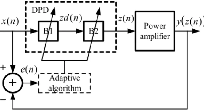
A structure of an adaptive DPD link to PA in accord-ance with the feedforward algorithm of DPD learning is shown in Fig. 1 [6]. Here, DPD is described by the nonlin-ear operator S composed of two nonlinnonlin-ear operators S1, S2, which are characteristic of two cascade connected blocks correspondently. The operators S1 and S2 are introduced in the operational equations
( )
)(n S1x n
zd , z(n)S2
zd(n)
,where n is the normalized discrete time, x(n), z(n) are the DPD input and output signals respectively, zd(n) is the output signal of the block described by the operator S1 and shown in Fig. 1.
Models of nonlinear operators S1 and S2 are con-structed by solving the approximation problem
x
n x n z y
N n min0, )
( ) (
B1 B2
+
)
(n
x
Power amplifier
)
(n
e
Adaptive algorithm
) (n z
)
(n
zd
DPD
z
(n
)
y
Fig. 1. The structure of the DPD feedforward learning algorithm.
where y(z(n)) is the PA output signal, Nx is the number of
samples of the input signal x(n). At first we build a model of the operator S1, followed by a model of the operator S2. Polynomials and neural networks can be used as nonlinear operator models
Parameters of cascade DPD nonlinear models are derived from the solution of the approximation problem (1) by iteration procedures under the following equations:
) ( ) ( ) (
1 n z n e n
zk k k , k1, ) ( ) ( ) (
1 n zd n e n
zdk k k , k1,
where k is the iteration number, ek(n) is the error of PA
linearization at the k-th iteration,
( )
)( )
(n x n y z n
ek k .
For k = 1 let us assume that
) ( ) ( )
( 1
1 n zd n x n
z .
PA has a low nonlinearity that is why its model can be represented as the convergent Volterra series. As a re-sult the predistorter is weakly nonlinear. This condition influences the quick convergence of the DPD synthesis iteration procedure.
At the cascade DPD synthesis the decomposition of the approximation problem (1) is carried out, i.e. the ap-proximation problem (1) with a high dimension is divided into two approximation problems with less dimensions solved in DPD blocks consecutively. Under this approach the ill conditionality problem of the approximation prob-lem (1) is solved.
We use FLANN [2–4] and PPN [4], [5] as models of the nonlinear operators S1 and S2.
3.
Functional Link Artificial Neural
Network
FLANN is a single-layer network [2–4]. Therefore the algorithm of this network learning has a more rapid convergence to the solution of the approximation problem and it is simpler in comparison with the algorithms of tra-ditional neural networks learning.
The FLANN model is expressed as
( )
( )
)(
1
n f
n w f n
y T
G
i i
i X W ΦX
(2)
where f is the nonlinear activation function of the network,
X(n) is the vector of input signals, X(n) = [x1(n), x2(n),…,
xQ(n)]T, T denotes transposing of the vector, W(n) is the
vector of network weights, W = [w1, w2,…, wG]T, (X(n))
is the vector of the functions i, (X(n)) =
[1(X(n)), 2(X(n)),…, G(X(n))]T, y(n) is the output
signal of the model.
The functions i, i = 1,2,…,G of the model (2)
trans-form input signals into basic functions by, for example, trigonometric polynomials, Legendre or Chebyshev poly-nomials and carry out a multidimensional transformation of the obtained basis functions. The basic functions are formed for reducing the condition number at solving high nonlinear approximation problem.
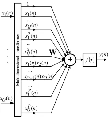
The FLANN structure is shown in Fig. 2.
Fu
nctiona
l li
n
k
)
(
1
n
x
1
w
2
w
+
f
)
(
2
n
x
)
(n
x
Q
(
)
1
X
n
(
)
2
X
n
(
n
)
G
X
w
G)
(n
y
.
.
.
.
.
.
Fig. 2. The FLANN structure.
For DPD synthesis let us consider the linear activa-tion funcactiva-tion f in the model (2) and the basic funcactiva-tions as Chebyshev polynomials Ti (X(n)) of degree i, i = 1,2,…,P
[2], [7]. From (2) we infer
( )
)(n n
y WT X (3)
where
X(n)
1,T1
x1(n)
,...,TQ
xQ(n)
,...,T2
x1(n)
,..., Φ
( )
,..., 1
1( )
1 2( )
,...,2 x n T x n T x n
T Q
TQ P P
Q
Q n T x n T x n T x n
x
T1 1( ) 1 ( ),..., 1( ),..., ( ) .
In the considered case the block named “Functional link” (Fig. 2) is represented as a structure showed in Fig. 3. The block “Functional link” consists of two blocks. In the first block Chebyshev polynomials of different degrees are formed on the bases of a variety of input signals, and the second block is the multidimensional transformation.
)
(
1
n
x
)
(n
x
Q.
.
.
1(
)
1
x
n
T
X
(n
)
Φ
.
.
.
x
1(
n
)
T
P
(
)
1
x
n
T
Q.
.
.
x
(n
)
T
P QM
u
lti
dimen
si
ona
l
tr
ansfo
rmati
o
n
Functional link
.
.
.
.
.
.
Fig. 3. The structure of the block “Functional link”.
First multiplier
2x2(n)–1
x(n)x(n–i)
2x2(n–i)–1
Second multiplier
x*(n)
x*(n–i)
Tab. 1. Multipliers of CFLANN members of the 3rd degree.
First multiplier
4x3(n)–3x(n)
4x3(n–i)–3x(n–i)
(2x2(n)–1) x(n–i)
(2x2(n–i)–1) x(n)
Second multiplier
(2x*(n))2–1
(2x*(n–i))2–1
x*( n)x*( n–i)
Tab. 2. Multipliers of CFLANN members of the 5th degree.
First multiplier
8x4(n)– 8x2(n)+1
8x4(n–i)– 8x2(n–i)+1
(2x2(n)–1) (2x2(n–i)–1)
x(n) (4x3(n–i)–3x(n–i))
x(n–i) (4x3(n)–3x(n))
Second multiplier
4(x*(n))3–3x*(n)
4(x*(n–i))3–3x*(n–i)
(2(x*(n))2–1)x*(n–i)
(2(x*(n–i))2–1)x*(n)
Tab. 3. Multipliers of CFLANN members of the 7th degree.
First multiplier
16x5(n)–20x3(n)+5x(n)
16x5(n–i)–20x3(n–i)+5x(n–i)
x(n)(8x4(n–i)–8x2(n–i)+1)
x(n–i)(8x4(n)–8x2(n)+1)
(4x3(n)–3x(n)) (2x2(n–i)–1)
(4x3(n–i)–3x(n–i)) (2x2(n)–1)
Second multiplier
8(x*(n))4–8 (x*(n))2+1
8(x*(n–i))4–8 (x*(n–i))2+1
(2(x*(n))2–1) (2(x*(n–i))2–1)
(4(x*(n))3–3x*(n))x*(n–i)
(4(x*(n–i))3–3x*(n–i))x*(n)
Tab. 4. Multipliers of CFLANN members of the 9th degree.
CFLANN of a predistorter should form an output signal spectrum located within the PA bandwidth at input signal frequencies and intermodulation frequencies of products generated by nonlinear PA [8].
The CFLANN model terms of odd (from the 1st to the 9th) degrees are produced by multiplying every components of the top columns from Tab. 1–4 by every components of
the corresponding bottom columns. In Tab. 1–4 the sign * means the complex conjugation, i is the signal delay.
The mentioned multiplication results in producing the vector (X(n)), which is then multiplied by the vector WT in (3). As a result we form the CFLANN model of odd degree.
4.
Polynomial Perceptron Network
PPN is a single-layer network [4], [5]. This network is characterized by the simplicity of its learning algorithm and high speed of convergence to the solution of the approximation problem.
The PPN model is described by the expression [4], [5]
( )
)
(n f n
y WTFX (4)
where f is the nonlinear activation function of the network,
X(n) is the vector of input signals, X(n) = [x1(n), x2(n),…,
xQ(n)]T, T denotes transposing of the vector, W(n) is the
vector of network weights, W = [w1, w2,…, wG]T, F(X(n))
is the vector containing elements with multidimensional transformation,
X(n)
1,x1(n),...,xQ(n),...,x12(n),...,xQ2(n),..., F
T P Q PQ
Q n x n x n x n
x n x n
x ( ) ( ),..., ( ) ( ),..., ( ),..., ( )
..., 1 2 1 1 ,
P is the degree of the function-vector element, y(n) is the output signal of the model (4).
The PNN structure is shown in Fig. 4.
+
f
y(n)M
u
ltidimens
io
n
al trans
former
) (
1 n
x
)
(n
x
Q) (
1 n
x
)
(n
x
Q) (
2 1 n
x
)
(
2
n
x
Q) ( ) ( 2
1 n x n
x
)
(
)
(
1
n
x
n
x
Q Q) (
1 n
xP
) (n xQP
1
...
...
...
...
...
W
. . .
From a comparison of PPN and FLANN it follows that FLANN (Fig. 2) is obtained from PPN (Fig. 4) by the additional transformation of input signals in basic functions by using Legendre polynomials, Chebyshev polynomials, etc.
For DPD synthesis let us assume that the activation function is linear in the model (4). We can rewrite (4) as
( )
)(n n
y WTFX . (5)
The input signal vector X(n) is formed on the basis of delay line. Multidimensional transformation F in the model (5) is performed under conditions of constructing inter-modulation spectral components of the DPD output [8], [9].
As a result we obtain the following PPN model
) ( ) ( )
(n y1 n y2 n
y (6)
where
2 / ) 1 ( 0 2 ) 1 ( 1 2 0
1( ) ( ) ( )
P k k k M i i n x w i n x n y
2 / ) 1 ( 1 2 ) 2 ( 1 2 1 ) ( ) ( P k k k M i n x w i n x
2 / ) 3 ( 0 2 ) 3 ( 3 2 2 0 * ) ( ) ( ) ( P k k k M i n x w n x i n x
M i k k P k i n x w i n x n x 1 2 ) 4 ( 3 2 2 / ) 3 ( 0 2 *( ) ( ) ( )
2 / ) 1 ( 1 2 ) 5 ( 1 2 1 ) ( ) ( P k k k M i i n x w n x
2 / ) 3 ( 0 2 ) 6 ( 3 2 0 *2( ) ( ) ( )
P k k k M i i n x w i n x n x
2 / ) 3 ( 0 2 ) 7 ( 3 2 0 2 ) ( ) ( ) ( P k k k M i i n x w i n x n x
M i k k P k i n x w i n x n x 0 2 ) 8 ( 5 2 2 / ) 5 ( 0 3 2 * ) ( ) ( )( , (7)
* is the sign of complex conjugation, M is the memory length, P is the odd degree of polynomial,
M i k k P k n x w n x i n x n y 1 2 ) 9 ( 5 2 2 / ) 5 ( 0 3 2 *2( ) ( ) ( ) ( )
M i k k P k n x w i n x n x 1 2 ) 10 ( 3 2 2 / ) 3 ( 1 2 * ) ( ) ( ) (
M i k k P k i n x w n x i n x 1 2 ) 11 ( 5 2 2 / ) 5 ( 1 3 2 *( ) ( ) ( )
M i k k P k n x w i n x n x 1 2 ) 12 ( 5 2 2 / ) 5 ( 1 3 2 * ) ( ) ( ) (
2 / ) 3 ( 1 2 ) 13 ( 3 2 1 2 ) ( ) ( ) ( P k k k M i i n x w n x n x
2 / ) 3 ( 1 2 ) 14 ( 3 2 1 2 ) ( ) ( ) ( P k k k M i n x w n x i nx . (8)
The expression (7) describes the radially pruned Volterra model (RPVM). RPVM is the regressive form of the trun-cated Volterra series. Volterra kernels in RPVM are built on a hypercube grid and radial directions are selected on the basis of the 3rd order kernel [9], [10].
5.
Compensation of Nonlinear
Distor-tion in PA Wiener-Hammerstein
Model
In practice a nonlinear PA exhibits a memory effect that is why a nonlinear predistorter with memory should be used for compensation of PA nonlinearity.
In the presented example, we assume the PA model is Wiener-Hammerstein model composed of a linear time-invariant (LTI) system, followed by a memoryless nonline-arity, which is in turn followed by another LTI system [9], [11]. The LTI blocks before and after the memoryless non-linearity have the system functions given by
1 2 1 2 . 0 1 5 . 0 1 ) ( z z z
H , 1
2 2 4 . 0 1 1 . 0 1 ) ( z z z H ,
correspondently. The memoryless nonlinear part of the described PA model is given by
4 5
2 3
1 ( ) ( ) ( ) ( ) ( )
)
(n bvn b v n vn b v n vn
w ,
where b11.01080.0858j, b30.08790.1583j, j
b51.09920.8891 , v(n) is the output signal of the LTI
system with the function H1(z).
The input signal for the PA model is the complex envelope of a GSM-signal with four carriers in the frequency baseband with the bandwidth of 20 MHz. The sampling frequency of the GSM-signal complex envelope is 184.32 MHz.
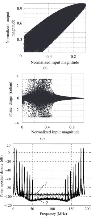
The dependences of the normalized magnitude and phase change of the PA output signal on the PA input sig-nal normalized magnitude are depicted in Fig. 5 (a), (b). In Fig.5 (c) the power spectral densities (PSD) of the de-scribed PA model input and output signals without DPD application are shown by dotted (1) and solid (2) lines correspondingly.
0.3 0.6 0.9
0
N
o
rm
al
ized out
p
ut
m
agni
tu
de
0.4 0.8
Normalized input magnitude (a)
0 0.4 0.8
Normalized input magnitude
4
0 2 4
P
h
ase
chage
(r
adi
an)
(b)
0 50 100 150 200
120
100
80
60
40
20 0 20
Frequency (MHz)
P
o
w
er s
p
ectr
al
d
ens
ity
(
d
B
)
1
2
(c)
Fig. 5. PA characteristics and signal PSD without DPD.
(7) and (8) are (P – 1)/2. The memory length of the inves-tigated models is 4 (M = 4 in (7), (8)).
The PA linearization error is estimated by normalized mean-square error (NMSE). This error is calculated from the expression
1
2
0
10 1
2
0
( ) ( )
10 log ,
( )
x
x
N n
N n
y z n x n NMSE
x n
dB,
where x(n) is the complex-valued input signal of the cas-cade connection between DPD and PA shown in Fig. 1, Nx
is the number of samples in the input signal x(n), Nx =
106339, y(z(n)) is the PA complex-valued output signal.
Model NMSE Q
CFLANN of the 9th degree –65.04 226
RPVM (7) at P = 7 –72.87 145
PPN (6) at P = 7 –75.50 221
Cascade connection
CFLANN of the 9th degree
and CFLANN of the 7th
degree
–69.42 375
RPVM (7) at P = 7 and
RPVM (7) at P = 7 –78.14 290
PPN (6) at P = 7 and
RPVM (7) at P = 7 –79.14 366
Tab. 5. NMSE and Q in DPD models.
NMSE estimated on the 45th iteration of the DPD adaptive algorithm and the number Q of coefficients in DPD models are presented in Tab. 5.
0.5 1
0
N
o
rm
al
ized out
put
m
agni
tude
0.5 1
Normalized input magnitude (a)
0 0.4 0.8
Normalized input magnitude
4
0 2 4
P
h
ase
chage
(r
adi
an)
(b)
0 50 100 150 200
120
100
80
60
40
20
0 20
Frequency (MHz)
P
o
w
er
s
p
ec
tr
al
dens
ity (
d
B
)
(c)
As can be seen from Tab. 5, the PPN model provides higher accuracy of PA linearization than RPVM and CFLANN. The use of the cascade DPD structure leads to an increased PA linearization accuracy. The highest accu-racy is achieved by the cascade DPD structure with PPN and RPVM.
Taking into account the cascade DPD with PPN and RPVM models the dependences of the normalized magni-tude and phase change of the PA output signal on the nor-malized magnitude of the DPD input signal are shown in Fig. 6 (a), (b). The PSD of the PA output signal at the mentioned cascade DPD is depicted in Fig. 6 (c).
From comparison of Fig. 6 with Fig. 5 it follows that the cascade DPD consisting of PPN and RPVM models gives a high quality of PA Wiener-Hammerstein model linearization.
6.
Conclusions
On the basis of the decomposition of the DPD nonlin-ear operator approximation problem into two sub-problems solved consecutively, it is possible to remove the ill condi-tionality from the DPD nonlinear operator approximation due to reduction of the approximation problem dimension.
This decomposition is realized in a cascade DPD synthesis. DPD block models are built as the functional link artificial neural network, the polynomial perceptron network and the radially pruned Volterra model.
DPD is synthesized for compensation of nonlinear distortion in PA Wiener-Hammerstein model at the com-plex envelope of a GSM-signal with four carriers. The predistortion results in the facts that the cascade DPD composed of PPN and RPVM linearizes PA with the high-est accuracy, and the cascade DPD based on CFLANN yields the lowest accuracy of PA linearization.
References
[1] LEGARDA, J. Feedforward Amplifiers for Wideband
Communication Systems. Dordrecht: Springer, 2006.
[2] LI, M., LIU, J., JIANG, Y., FENG, W. Complex-Chebyshev
func-tional link neural network behavioral model for broadband
wire-less power amplifiers. IEEE Transactions on Microwave Theory
and Techniques, 2012, vol. 60, no. 6, part 2, p. 1979–1989. DOI: 10.1109/TMTT.2012.218923
[3] PATRA, J. C., PAL, R. N., CHATTERJI, B. N., PANDA G.
Identification of nonlinear dynamic systems using functional link
artificial neural networks. IEEE Transactions on Systems, Man and
Cybernetics – Part B: Cybernetics, 1999, vol. 29, no. 2, p. 254 to 262. DOI: 10.1109/3477.752797
[4] PATRA, J. C., PAL, R. N., BALIARSINGH, R., PANDA G.
Nonlinear channel equalization for QAM signal constellation using
artificial neural networks. IEEE Transactions on Systems, Man and
Cybernetics – Part B: Cybernetics, 1999, vol. 29, no. 2, p. 262 to 271. DOI: 10.1109/3477.752798
[5] XIANG, Z., BI, G., LE-NGOC, T. Polynomial-perceptrons and
their applications to fading channel equalization and co-channel
interference suppression. IEEE Transactions on Signal Processing,
1994, vol. 42, no. 9, p. 2470–2480. DOI: 10.1109/78.317868
[6] ZHOU, D., DEBRUNNER, V. E. Novel adaptive nonlinear
pre-distorters based on the direct learning algorithm. IEEE
Transac-tions on Signal Processing, 2007, vol. 55, no. 1, p. 120–133. DOI: 10.1109/TSP.2006.882058
[7] LEE, T. T., JIANG, J. T. The Chebyshev polynomial based unified
model neural networks for function approximations. IEEE
Transactions on Systems, Man and Cybernetics – Part B: Cybernetics, 1998, vol. 28, no. 6, p. 925–935. DOI: 10.1109/3477.735405
[8] ZHOU, G. T., QIAN, H., DING, L., RAICH, R. On the baseband
representation of a bandpass nonlinearity. IEEE Transactions on
Signal Processing, 2005, vol. 53, no. 8, p. 2953–2957. DOI: 10.1109/TSP.2005.850383
[9] SOLOVYEVA, E. B. Dynamic deviation Volterra predistorter designed for linearizing power amplifiers. Radioelectronics and Communications Systems, 2011, vol. 54, no. 10, p. 546–553. DOI: 10.3103/S0735272711100049
[10] CRESPO-CADENAS, C., REINA-TOSINA, J.,
MADERO-AYORA, M. J., MUNOZ-CRUZADO, J. A new approach to
pruning Volterra models for power amplifiers. IEEE Transactions
on Signal Processing, 2010, vol. 58, no. 4, p. 2113–2120. DOI: 10.1109/TSP.2009.2039815
[11] DING, L., ZHOU, G. T., MORGAN, D. R., MA, Z., KENNEY, J.
S., KIM, J., GIARDINA, C. R. A robust digital baseband
pre-distorter constructed using memory polynomials. IEEE
Transac-tions on CommunicaTransac-tions, 2004, vol. 52, no. 1, p. 159–165. DOI: 10.1109/TCOMM.2003.822188