Design of Fuzzy Neural Network for Function
Approximation and Classification
Amit Mishra, Zaheeruddin
∗†Abstract— A hybrid Fuzzy Neural Network (FNN)
system is presented in this paper. The proposed FNN can handle numeric and fuzzy inputs simulta-neously. The numeric inputs are fuzzified by input nodes upon presentation to the network while the fuzzy inputs do not require this translation. The connections between input to hidden nodes repre-sent rule antecedents and hidden to output nodes represent rule consequents. All the connections are represented by Gaussian fuzzy sets. The mutual subsethood measure for fuzzy sets that indicates the degree to which the two fuzzy sets are equal and is used as a method of activation spread in the network. A volume based defuzzification method is used to compute the numeric output of the network. The training of the network is done using gradient descent learning procedure. The model has been tested on three benchmark problems i.e. sine−cosine and Narazaki Ralescu’s function for approximation and Iris flower data for classification. Results are also compared with existing schemes and the proposed model shows its natural capability as a function approximator, and classifier.
Keywords: Cardinality, classifier, function ap-proximation, fuzzy neural system, mutual subsethood
1
Introduction
The conventional approaches to system modeling that are based on mathematical tools (i.e. difference equations) perform poorly in dealing with complex and uncertain systems. The basic reason is that, most of the time; it is very difficult to find a global function or analytical struc-ture for a nonlinear system. In contrast, fuzzy logic pro-vides an inference morphology that enables approximate human reasoning capability to be applied in a fuzzy infer-ence system. Therefore, a fuzzy inferinfer-ence system employ-ing fuzzy logical rules can model the quantitative aspects of human knowledge and reasoning processes without em-ploying precise quantitative analysis.
∗Jaypee Institute of Engineering and Technology, A.B. Road,
Raghogarh, Distt.Guna, Madhya Pradesh, India, PIN-473226. Email: amitutk@ gmail.com
†Jamia Millia Islamia (A Central University), Department of
Electrical Engineering, Jamia Nagar, New Delhi, India, PIN-110 025. Email: zaheer 2k@ hotmail.com
In recent past, artificial neural network has also played an important role in solving many engineering problems [1], [2]. Neural network has advantages such as learning, adaption, fault tolerance, parallelism, and generalization. The fuzzy system utilizing the learning capability of neu-ral networks can successfully construct the input output mapping for many applications [3], [4]. The benefits of combining fuzzy logic and neural network have been ex-plored extensively in the literature [5], [6], [7], [8], [9]. The term neuro-fuzzy system (also neuro-fuzzy methods or models) refers to combinations of techniques from neu-ral networks and fuzzy system [10], [11], [12], [13], [14]. This does not mean that a neural network and a fuzzy system are used in some kind of combination, but a fuzzy system is created from data by some kind of (heuristic) learning method, motivated by learning procedures used in neural networks. The neuro-fuzzy methods are usually applied, if a fuzzy system is required to solve a problem of function approximation−or a special case of it, like, control or classification [15], [16], [17], [18], [19]−and the otherwise manual design process should be supported and replaced by an automatic learning process.
In this paper, the attention has been focused on the func-tion approximafunc-tion and classificafunc-tion capabilities of the subsethood based fuzzy neural model (subsethood based FNN). This model can handle simultaneous admission of fuzzy or numeric inputs along with the integration of a fuzzy mutual subsethood measure for activity propa-gation. A product aggregation operator computes the strength of firing of a rule as a fuzzy inner product and works in conjunction with volume defuzzification to gen-erate numeric outputs. A gradient descent algorithm al-lows the model to fine tune rules with the help of numeric data.
The organization of the paper is as follows: Section 2 presents the architectural and operational detail of the model. Section 3 describes the gradient descent learning procedure for training the model. Section 4 and Section 5 shows the experiment results for three benchmark prob-lems based on function approximation and classification. Finally, the Section 6 concludes the paper.
2
Fuzzy Neural Network system
x1
xi
xm
xm+1
xn
Input Layer Rule Layer Output Layer
Numeric nodes
Linguistic nodes
y1
yk
yp (cij, σij)
(cnj, σnj)
(cjk, σjk)
(cqk, σqk)
Antecedent connection
consequent connection
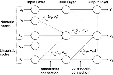
Figure 1: Architecture of subsethood based FNN model.
xm+1toxnare numeric and linguistic inputs respectively.
Each hidden node represents a rule, and input-hidden node connection represents fuzzy rule antecedent. Each hidden-output node connection represents a fuzzy rule consequent. Fuzzy set corresponding to linguistic levels of fuzzy if-then rules are defined on input and output UODs and are represented by symmetric Gaussian mem-bership functions specified by a center c and spread σ. The center and spread of fuzzy weights wij from input
nodes i to rule nodes j are shown as cij and σij of a
Gaussian fuzzy set and denoted bywij = (cij, σij). In a
similar way, consequent fuzzy weights from rule nodesj
to output nodesk are denoted byvjk = (cjk, σjk). Here
y1 to yk. . . yp are the outputs of the subsethood based
FNN model.
2.1
Signal Transmission at Input Nodes
In the proposed FNN the input featuresx1, ..., xn can be
either linguistic or numeric or the combination of both. Therefore two kinds of nodes may present in the input layer of the network corresponding to the nature of input features.
Linguistic nodes accept the linguistic inputs represented by a fuzzy sets with a Gaussian membership function and modeled by a centerciand spreadσi. These linguistic
in-puts can be drawn from pre-specified fuzzy sets as shown in Fig. 2, where three Gaussian fuzzy sets have been de-fined on the universe of discourse (UODs) [-1,1]. Thus, a linguistic input featurexi is represented by the pair of
center and spread (ci, σi). No transformation of inputs
takes place at linguistic nodes in the input layer. They merely transmit the fuzzy input forward along antecedent weights.
Numeric nodes accept numeric inputs and fuzzify them into Gaussian fuzzy sets. The numeric input is fuzzi-fied by treating it as the centre of a Gaussian member-ship function with a heuristically chosen spread. An ex-ample of this fuzzification process is shown in Fig. 3, where a numeric feature value of 0.3 has been fuzzified
-1 -0.5 0 0.5 1
0 0.1 0.2 0.3 0.4 0.5 0.6 0.7 0.8 0.9 1
LOW MEDIUM HIGH
Figure 2: Fuzzy sets for fuzzy inputs.
-1 -0.5 0 0.5 1
0 0.1 0.2 0.3 0.4 0.5 0.6 0.7 0.8 0.9 1
Fuzzified input Gaussian m.f. Center=0.3 Spread=0.35
Figure 3: Fuzzification of numeric input.
into a Gaussian membership function centered at 0.3 with spread 0.35. The Gaussian shape is chosen to match the Gaussian shape of weight fuzzy sets since this facilitates subsethood calculations detailed in section 2.2.
Therefore, the signal from a numeric node of the input layer is represented by the pair (ci, σi). Antecedent
con-nections uniformly receive signals of the form (ci, σi).
Signals (S(xi) = (ci, σi)) are transmitted to hidden rule
nodes through fuzzy weightswijalso of the form (cij, σij),
where single subscript notation has been adopted for the input sets and the double subscript for the weight sets.
2.2
Signal Transmission from Input to Rule
Nodes (Mutual Subsethood Method)
Since both the signal and the weight are fuzzy sets, being represented by Gaussian membership function, there is a need to quantify the net value of the signal transmitted along the weight by the extent of overlap between the two fuzzy sets. This is measured by theirmutual subsethood
[20]. Consider two fuzzy setsAandB with centersc1, c2
and spreadsσ1, σ2respectively. These sets are expressed
by their membership functions as:
a(x) =e−((x−c1)/σ1)2. (1)
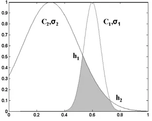
Figure 4: Example of overlapping: c1> c2 andσ1< σ2.
ithinput node (numeric or linguistic)
jthrule node
εij Fuzzy signal
S(xi)=(ci, σi)
Fuzzy weight wij=(cij, σij) Mutual subsethood
Xi
Figure 5: Fuzzy signal transmission.
The cardinalityC(A) of fuzzy set Ais defined by
C(A) =
Z ∞
−∞
a(x)dx=
Z ∞
−∞
e−((x−c1)/σ1)2dx. (3)
Then the mutual subsethoodE(A, B) of fuzzy setsAand
B measures the extent to which fuzzy setAequals fuzzy set B can be evaluated as:
E(A, B) = C(A∩B)
C(A) +C(B)−C(A∩B). (4)
Further detail on the mutual subsethood measure can be found in [20]. Depending upon the relative values of centers and spreads of fuzzy sets A and B (nature of overlap), the four possible different cases are as follows: case 1: c1=c2having any values ofσ1and σ2.
case 2: c16=c2andσ1=σ2.
case 3: c16=c2andσ1> σ2.
case 4: c16=c2andσ1< σ2.
In case 1, the two fuzzy sets do not cross over−either one fuzzy set belongs completely to the other or two fuzzy sets are identical. In case 2, there is exactly one cross over point, whereas in cases 3 and 4, there are exactly two crossover points. An example of case 4 type overlap is shown in Fig. 4. To calculate the crossover points, by setting a(x) =b(x), the two cross over points h1 andh2
yield as,
h1=
c1+σσ1 2c2
1 + σ1
σ2
, (5)
h2=
c1−σσ1 2c2
1−σ1
σ2
. (6)
These values ofh1andh2are used to calculate the mutual
subsethoodE(A, B) based onC(A∩B), as defined in (4). Symbolically, for a signal si=S(xi) = (ci, σi) and fuzzy
weightwij = (cij, σij), the mutual subsethood is
Eij =E(si, wij) =
C(si∩wij)
C(si) +C(wij)−C(si∩wij)
. (7)
As shown in Fig. 5, in the subsethood based FNN model, a fuzzy input signal is transmitted along a fuzzy weight that represents an antecedent connection. The transmit-ted signal is quantified by Eij, which denotes the
mu-tual subsethood between the fuzzy signalS(xi) and fuzzy
weight (cij, σij) and can be computed using (4).
The expression for cardinality can be evaluated for each of the four cases in terms of standard error functionerf(x) represented as (8).
erf(x) =√2
π
Z x
0
e−t2
dt. (8)
The expressions forC(si∩wij) for all the four cases
iden-tified above are evaluated in Appendix (A) seperately.
2.3
Activity Aggregation at Rule Nodes
(Product Operator)
The net activation zj of the rule node j is a product of
all mutual subsethoods known as the fuzzy inner product can be evaluated as
zj = n
Y
i=1
Eij = n
Y
i=1
E(S(xi), wij) (9)
The inner product operator in (9) exhibits following prop-erties: it is bounded between 0 and 1; monotonic increas-ing; continuous and symmetric.
The signal function for the rule node is linear
S(zj) =zj. (10)
Numeric activation values are transmitted unchanged to consequent connections.
2.4
Output Layer Signal Computation
(Vol-ume Defuzzification)
The signal of each output node is determined using stan-dard volume based centroid defuzzification [20]. The ac-tivation of the output node is yk, and Vjk’s denote
con-sequent set volumes, then the general expression of de-fuzzification is
yk=
Pq
j=1zjcjkVjk
Pq
j=1zjVjk
The volume Vjk is simply the area of consequent fuzzy
sets which are represented by Gaussian membership func-tion. From (11), the output can be evaluated as
yk=
Pq
j=1zjcjkσjk
Pq
j=1zjσjk
. (12)
The signal of output nodek is linear i.e. S(yk) =yk.
3
Supervised learning (Gradient descent
algorithm)
The subsethood based linguistic network is trained by su-pervised learning. This involves repeated presentation of a set of input patterns drawn from the training set. The output of the network is compared with the desired value to obtain the error, and network weights are changed on the basis of an error minimization criterion. Once the network is trained to the desired level of error, it is tested by presenting a new set of input patterns drawn from the testing set.
3.1
Update Equations for Free Parameters
Learning is incorporated into the subsethood−linguistic model using the gradient descent method [15], [21]. A squared error criterion is used as a training performance parameter. The squared error et at iteration t is
com-puted in the standard way
et= 1 2
p
X
k=1
(dtk−S(ytk))2. (13)
where dt
k is the desired value at output node k, and the
error evaluated over all poutputs for a specific pattern
k. Both the centers and spreads cij, cjk, σij and σjk of
antecedents and consequent connections are modified on the basis of update equations given as follows:
ctij+1=ctij−η
∂et
∂ct ij
+α△ctij−1. (14)
whereη is the learning rate,αis the momentum param-eter, and
△ctij−1=cijt −ctij−1. (15)
3.2
Partial Derivatives Evaluation
The expressions of partial derivatives required in these update equations are derived as follows:
For the error derivative with respect to consequent cen-ters
∂e ∂cjk
= ∂e
∂yk
∂yk
∂cjk
=−(dk−yk)
zjσjk
Pq
j=1zjσjk
(16)
and the error derivative with respect to the consequent spreads
∂e ∂σjk
= ∂e
∂yk
∂yk
∂σjk
= −(dk−yk)
(
zjcjkPqj=1zjσjk−zjPqj=1zjcjkσjk
(Pq
j=1zjσjk)2
)
.
(17)
The error derivatives with respect to antecedent centers and spreads involve subsethood derivatives in the chain and are somewhat more involved to evaluate. Specifically, the error derivative chains with respect to antecedent cen-ters and spreads are given as following,
∂e ∂cij
=
p
X
k=1
∂e ∂yk
∂yk
∂zj
∂zj
∂Eij
∂Eij
∂cij
=
p
X
k=1
−(dk−yk)
∂yk
∂zj
∂zj
∂Eij
∂Eij
∂cij
, (18)
∂e ∂σij
=
p
X
k=1
∂e ∂yk
∂yk
∂zj
∂zj
∂Eij
∂Eij
∂σij
=
p
X
k=1
−(dk−yk)
∂yk
∂zj
∂zj
∂Eij
∂Eij
∂σij, (19)
and the error derivative chains with respect to input fea-ture spread is evaluated as
∂e ∂σi
=
q
X
j=1
p
X
k=1
∂e ∂yk
∂yk
∂zj
∂zj
∂Eij
∂Eij
∂σi
=
q
X
j=1
p
X
k=1
−(dk−yk)
∂yk
∂zj
∂zj
∂Eij
∂Eij
∂σi
. (20)
where
∂yk
∂zj
= σjkcjk
Pq
j=1zjσjk−σjkPqj=1zjcjkσjk
(Pq
j=1zjσjk)2
= σjk
"
cjkPqj=1zjσjk−Pqj=1zjcjkσjk
(Pq
j=1zjσjk)2
#
= σPjkq(cjk−yk)
j=1zjσjk
(21)
and
∂zj
∂Eij
=
n
Y
i=1,i6=j
Eij. (22)
The expressions for antecedent connection, mutual sub-sethood partial derivatives ∂Eij
∂cij and
∂Eij
∂σij are obtained by differentiating (7) with respect to cij, σij and σi as in
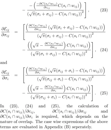
(23), (24) and (25). In these equations, the calculation of ∂C(si∩wij)/∂cij and ∂C(si∩wij)/∂σij depends on
the nature of overlap of the input feature fuzzy set and weight fuzzy set, i.e. upon the values ofcij, ci, σijandσi.
∂Eij
∂cij
=
³∂C(s
i∩wij)
∂cij (
√
π(σi+σij)−C(si∩wij))
´
− − ³−∂C(s
i∩wij)
∂cij C(si∩wij)
´
(√π(σi+σij)−C(si∩wij))
2
, (23)
∂Eij
∂σij
=
³∂C(s
i∩wij)
∂σij (
√
π(σi+σij)−C(si∩wij))
´
(√π(σi+σij)−C(si∩wij))
2
− ³³√
π−∂C(si∩wij)
∂σij
´
C(si∩wij)
´
(√π(σi+σij)−C(si∩wij))
2
, (24)
and
∂Eij
∂σi
=
³∂C(s
i∩wij)
∂σi (
√
π(σij+σi)−C(si∩wij))
´
(√π(σij+σi)−C(si∩wij))2
− ³³√
π−∂C(si∩wij)
∂σi
´
C(si∩wij)
´
(√π(σij+σi)−C(si∩wij))2
. (25)
In (23), (24) and (25), the calculation of
∂C(si∩wij)/∂cij, ∂C(si∩wij)/∂σij and
∂C(si∩wij)/∂σi is required, which depends on the
nature of overlap. The case wise expressions of the above terms are evaluated in Appendix (B) seperately.
4
Function approximation
Function approximation involves determining or learning the input-output relations using numeric input-output data. Conventional methods like linear regression are useful in cases where the relation being learnt, is linear or quasi-linear. For nonlinear function approximation multi-layer neural networks are well suited to solve the problem but at the same time they also experience the drawback of their black box nature and heuristic decisions regard-ing the network structure and tunable parameters. Inter-pretability of learnt knowledge is another severe problem in conventional neural networks.
On the other hand, function approximation by fuzzy sys-tem employs the concept of dividing the input space into sub regions, and for each sub region a fuzzy rule is de-fined thus making the system interpretable. The perfor-mance of the fuzzy system depends on the generation of sub regions in input space for a specific problem. The practical limitation arises with fuzzy systems when the input variables are increased and the number of fuzzy rules explodes leading to the problem known as the curse of dimensionality.
Both fuzzy system and neural network are universal func-tion approximators and can approximate funcfunc-tions to any arbitrary degree of accuracy [20], [22]. Fuzzy neural sys-tem also has capability of approximating any continuous function or modeling a system [23],[24],[25]. The pro-posed fuzzy neural network was tested to exploit the ad-vantages of both neural network and fuzzy system seam-lessly in the applications like function approximation and classification.
0 2
4 6
8
0 2 4 6 8 -1 -0.5 0 0.5 1
x y
f(
x
,y
)
(a)
0 2
4 6
8
0 2 4 6 8 -1 -0.5 0 0.5 1
x y
f(
x
,y
)
(b)
Figure 6: (a) Mesh plot and contours of 900 training pat-terns. (b) Mesh plot and contours of 400 testing patpat-terns.
Table 1: Details of different learning schedules used for simulation studies
Learning Schedule Details
LS=0.2 ηandαare fixed to 0.2 LS=0.1 ηandαare fixed to 0.1 LS=0.01 ηandαare fixed to 0.01 LS=0.001 ηandαare fixed to 0.001
η-learning rate andα-momentum
4.1
Sine-Cosine Function
The learning capabilities of the proposed model was demonstrated by approximating thesine-cosine function given as
f(x, y) =sin(x)cos(y). (26)
for the purpose of training the network the above func-tion was described by 900 sample points, evenly dis-tributed in a 30x30 grid in the input cross-space [0,2π] x[0,2π]. The model was tested by another set of 400 points evenly distributed in a 20x20 grid in the input cross-space [0,2π]x[0,2π]. The mesh plot of training and testing patterns are shown in Fig. 6.
0 2 4 6 8 0 2 4 6 8 -1 -0.5 0 0.5 1 x y f( x ,y ) (a) 0 2 4 6 8 0 2 4 6 8 -1 -0.5 0 0.5 1 x y f( x ,y ) (b) 0 2 4 6 8 0 2 4 6 8 -1 -0.5 0 0.5 1 x y f( x ,y ) (c) 0 2 4 6 8 0 2 4 6 8 -1 -0.5 0 0.5 1 x y f( x ,y ) (g) 0 2 4 6 8 0 2 4 6 8 -1 -0.5 0 0.5 1 x y f( x ,y ) (h) 0 2 4 6 8 0 2 4 6 8 -1 -0.5 0 0.5 1 x y f( x ,y ) (i) 0 2 4 6 8 0 2 4 6 8 -1 -0.5 0 0.5 1 x y te s ti n g e rr o r (d) 0 2 4 6 8 0 2 4 6 8 -1 -0.5 0 0.5 1 x y te s ti n g e rr o r (e) 0 2 4 6 8 0 2 4 6 8 -1 -0.5 0 0.5 1 x y te s ti n g e rr o r (f) 0 2 4 6 8 0 2 4 6 8 -1 -0.5 0 0.5 1 x y te s ti n g e rr o r (j) 0 2 4 6 8 0 2 4 6 8 -1 -0.5 0 0.5 1 x y te s ti n g e rr o r (k) 0 2 4 6 8 0 2 4 6 8 -1 -0.5 0 0.5 1 x y te s ti n g e rr o r (l)
Figure 7: f(x, y) surace plot and their corresponding testing error surface after 250 epochs for different rule counts with learning schedule LS=0.01, (a)f(x, y) surface for 5 rules, (b)f(x, y) surface for 10 rules, (c)f(x, y) surface for 15 rules, (d) error suface for 5 rules, (e) error suface for 10 rules, (f) error suface for 15 rules, (g)f(x, y) surface for 20 rules, (h)f(x, y) surface for 30 rules, (i)f(x, y) surface for 50 rules, (j) error suface for 20 rules, (k) error suface for 30 rules, (l) error suface for 50 rules.
between rule layer and output layer were initially ran-domized in the range [−1,1]. The spreads of all the fuzzy weights and the spreads of input feature fuzzifiers were initialized randomly in range [0.2,0.9].
The number of free parameters that subsethood based FNN employs is straightforward to calculate: one spread for each numeric input; a center and a spread for each antecedent and consequent connection of a rule. For this function model employs a 2-r-1 network architec-ture, where r is the number of rule nodes. Therefore, since each rule has two antecedents and one consequent, an r-rule FNN system will have 6r+2 free parameters. Model was trained for different number of rules−5, 10, 15, 20, 30 and 50. To study the effect of learning param-eters on the performance of model the simulation were performed with different learning schedules as shown in Table 1 . The root mean square error, evaluated for both training and testing patterns, is given as
RM SEtrn=
s P
training patterns(desired−actual)2
number of training patterns
(27)
RM SEtest=
s P
testing patterns(desired−actual)2
number of testing patterns
(28)
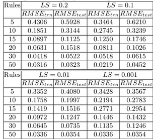
Table 2: Root mean square errors for different rule count and learning schedules (LS) for 250 epochs
Rules LS= 0.2 LS= 0.1
RM SEtrnRM SEtestRM SEtrnRM SEtest
5 0.4306 0.5928 0.3464 0.6210 10 0.1851 0.3144 0.2745 0.3239 15 0.0897 0.1125 0.1250 0.1746 20 0.0631 0.1518 0.0811 0.1026 30 0.0418 0.0522 0.0518 0.0615 50 0.0316 0.0323 0.0219 0.0452 Rules LS= 0.01 LS= 0.001
RM SEtrnRM SEtestRM SEtrnRM SEtest
5 0.3352 0.4080 0.3428 0.3567 10 0.1758 0.1997 0.2194 0.2783 15 0.1419 0.1516 0.2771 0.2954 20 0.0972 0.1247 0.1446 0.1432 30 0.0645 0.0735 0.1135 0.1246 50 0.0336 0.0354 0.0336 0.0354
0 50 100 150 200 250 300 350 400 450 500 0
0.05 0.1 0.15 0.2 0.25 0.3 0.35 0.4 0.45 0.5
epochs
te
s
ti
n
g
e
rr
o
r
LS=0.2
5 rules 10 rules 15 rules 20 rules 30 rules 50 rules
0 50 100 150 200 250 300 350 400 450 500 0
0.05 0.1 0.15 0.2 0.25 0.3 0.35 0.4 0.45 0.5
epochs
te
s
ti
n
g
e
rr
o
r
LS=0.1
5 rules 10 rules 15 rules 20 rules 30 rules 50 rules
0 50 100 150 200 250 300 350 400 450 500 0
0.1 0.2 0.3 0.4 0.5 0.6 0.7
epochs
te
s
ti
n
g
e
rr
o
r
LS=0.01
5 rules 10 rules 15 rules 20 rules 30 rules 50 rules
0 50 100 150 200 250 300 350 400 450 500 0.1
0.2 0.3 0.4 0.5 0.6 0.7 0.8
epochs
te
s
ti
n
g
e
rr
o
r
LS=0.001
5 rules 10 rules 15 rules 20 rules 30 rules 50 rules
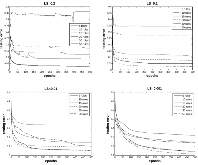
Figure 8: Error trajectories for different rules and learning schedules insine−cosinefunction problem.
the given function. The error is more where the slope of the function changes in that region. Thus, increasing the number of rules generates better approximated surface forf(x, y) and the corresponding plots are shown in Fig. 7.
From the results shown in Table 2 it is observed that for a learning schedule LS=0.2 or higher and with small rule count the subsethood model is unable to train, result-ing oscillations in error trajectories as shown in Fig. 8. This may occur due to the improper selection of learning parameters (learning rate (η) and momentum (α)) and number of rules. But with the same learning parameters and higher rule counts like 30 and 50 rules model pro-duces good approximation. The observations for fuzzy neuro model drawn in the above experiments can be sum-marized as following:
1. As the number of rules increases the approximation performance of model improves to a certain limit. 2. For higher learning rates and momentum with lower rule counts the model is unable to learn. In contrast if the learning rate and momentum are kept to small values a smooth decaying trajectory is obtained even for small rule counts.
3. Model works fairly well by keeping the learning rate and momentum fixed to small values.
4. Most of the learning is achieved in a small number of epochs.
4.2
Narazaki and Ralescu function
The function is expressed as follows,
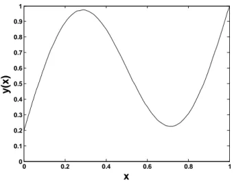
y(x) = 0.2 + 0.8(x+ 0.7sin(2πx)),0≤x≤1 (29)
and the plot of the function is shown in Fig.9. The system architecture used for approximating single input-output function is 1-r-1, where r is the number of rule nodes. The tunable parameters that model employs for this application can be calculated same as the sine−
cosine function i.e. one spread for each input, and a center and a spread for each antecedent and consequent connection of rule. As each rule has one antecedent and one consequent, r rule architecture will have 4r+1 free parameters. The model was trained using 21 training patterns. These patterns were generated at intervals of 0.05 in range [0,1]. Thus, the training patterns are of the form:
0 0.2 0.4 0.6 0.8 1 0
0.1 0.2 0.3 0.4 0.5 0.6 0.7 0.8 0.9 1
x
y
(x
)
Figure 9: Narazaki-Ralescu function.
The evaluation was done using 101 test data taken at intervals of 0.01. The training and test sets generated were mutually exclusive. Two performance indices J1 and J2 as defined in [26], used for evaluation are given as:
J1 = 100×211 X
training data
|actual output−desired output|
desired output
(31)
J2 = 100×1011 X
test data
|actual output−desired output|
desired output
(32) Experiments were conducted for different rule counts, using a learning rate of 0.01 and momentum of 0.01 throughout the learning procedure. Table 3 summarizes the performance of model in terms of indices J1 and J2 for rule counts 3 to 6. It is evident from the performance measures that for 5 or 6 rules the approximation accu-racy is much better than that for 3 or 4 rules. In general up to a certain limit, as the number of rules grows, the performance of model improves.
Table 4 compares the test accuracy performance indexJ2 for different models along with the number of rules and tunable parameters used to achieve it. With five rules the proposed model obtained J1 = 0.9467 andJ2 = 0.7403 as better than other schemes. From the above results, it can be infer that subsethood-based FNN shows the ability to approximate function with good accuracy in comparison with other existing models.
Table 3: Subsethood based FNN performance for Narazaki-Ralescu’s function
Number Trainable Training Testing of Rules Parameter Accuracy (J1%) Accuracy (J2%)
3 13 2.57 1.7015 4 17 1.022 0.7350 5 21 0.94675 0.7403 6 25 0.6703 0.6595
Table 4: Performance comparison of subsethood based FNN with other methods for Narazaki-Ralescu’s function
Methods Number Trainable Testing and reference of RulesParametersAccuracy (J2%) FuGeNeSys[31] 5 15 0.856 Lin and Cunningham III [32] 4 16 0.987 Narazaki and Ralescu[26] na 12 3.19 Subsethood based FNN 3 13 1.7015 Subsethood based FNN 5 21 0.7403
Table 5: Iris data classification results for the subsethood based Fuzzy Neural Network system
Rule Free RMSE number of resubstitution Count Parameters mis-classifications accuracy (%)
3 46 0.12183 1 99.33
4 60 0.12016 0 100
5 74 0.11453 0 100
6 88 0.11449 0 100
7 102 0.11232 0 100 8 116 0.10927 0 100
5
Classification
In classification problems, the purpose of the proposed network is to assign each pattern to one of a number of classes (or, more generally, to estimate the probability of membership of the case in each class). The Iris flower data set or Fisher’s Iris data set is a multivariate data set introduced by Sir Ronald Aylmer Fisher as an example of discriminant analysis.
5.1
Iris data Classification
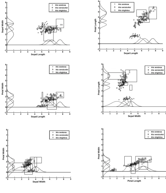
Iris data involves classification of three subspecies of the flower namely, Iris sestosa, iris versicolor and Iris vir-ginica on the basis of four feature measurements of the Iris flower-sepal length, sepal width, petal length and petal width [27]. There are 50 patterns (of four features) for each of the three subspecies of Iris flower. The in-put pattern set thus comprises 150 four-dimensional pat-terns. This data can be obtained from UCI repository of machine learning databases through the following link−
http://www.ics.uci.edu/ mlearn/M LRepository.html. The six possible scatter plots of Iris data are shown in Fig. 10. It can be observed that classesIris versicolor andIris virginica substantially overlap, while class Iris sestosais well separated from the other two. For this classification problem subsethood based FNN model employs a 4-r-3 network architecture: the input layer consists of four nu-meric nodes; the output layer comprises three class nodes; and there are r rule nodes in the hidden layer.
4 4.5 5 5.5 6 6.5 7 7.5 8 2
2.5 3 3.5 4 4.5 5
Sepal Length
S
e
p
a
l
W
id
th
4 4.5 5 5.5 6 6.5 7 7.5 8 0
1 2 3 4 5 6 7 8
Sepal Length
P
e
ta
l
L
e
n
g
th
Iris sestosa Iris versicolor Iris virginica
4 4.5 5 5.5 6 6.5 7 7.5 8 0
0.5 1 1.5 2 2.5 3
Sepal Length
P
e
ta
l
W
id
th
2 2.5 3 3.5 4 4.5
0 1 2 3 4 5 6 7 8
Sepal Width
P
e
ta
l
L
e
n
g
th
2 2.5 3 3.5 4 4.5
0 0.5 1 1.5 2 2.5 3
Sepal Width
P
e
ta
l
W
id
th
0 1 2 3 4 5 6 7 8
0 0.5 1 1.5 2 2.5 3
Petal Length
P
e
ta
l
W
id
th
Figure 10: Six projection plots of Iris data.
range (0,1) and the spreads of all fuzzy weights and fea-ture spreads were randomized in the range (0.2, 0.9). All 150 patterns of the Iris data were presented sequentially to the input layer of the network for training. The learn-ing rate and momentum were kept constant at 0.001 dur-ing the traindur-ing process. The test patterns which again comprised all 150 patterns of Iris data were presented to the trained network and the resubstitution error com-puted.
Simulation experiments were conducted with different numbers of rule nodes to illustrate the performance of the classifier with a variation in the number of rules. No-tice that for r rules, the number of connections in the 4-r-3 architecture for Iris data will be 7r. Because the representation of a fuzzy weight requires two parameters (center and spread), the total number of free parameters to be trained will be 14r+4.
Table 5 summarizes the performance of proposed model for different rule counts. It is observed that except for rule
count 3 subsethood based FNIS model is able to achieve 100 % resubstitution accuracy by classifying all patterns correctly. Thus by merely using 60 parameters for subset-hood based FNN model produces no mis-classifications, and using only 46 free parameters 1 mis-classification is obtained. Apart from this, it is also observed from Table 5 that as the numbers of rules increase the training root mean square error (RMSE) decreases.
As an example, the fuzzy weights of the trained network with four rules that produce zero resubstitution error are illustrated in the scatter plot of Iris data in Fig. 11. The rule patches in two dimensions were obtained by finding the rectangular overlapping area produced by the projec-tion of 3σ points of the Gaussian fuzzy sets on different input feature axes of the same rule. The 3σpoints were chosen because for 3σon either side of centers of a Gaus-sian fuzzy set 99.7 % of the total area of the fuzzy set gets covered.
0 1 2 3 4 5 6 7 8 9 -1
0 1 2 3 4 5 6 7 8
Sepal Length
S
e
p
a
l
W
id
th
Iris sestosa Iris versicolor Iris virginica
0 1 2 3 4 5 6 7 8 9
-1 0 1 2 3 4 5 6 7
Sepal Length
P
e
ta
l
L
e
n
g
th
Iris sestosa Iris versicolor Iris virginica
0 1 2 3 4 5 6 7 8 9
-1 0 1 2 3 4 5 6 7 8
Sepal Length
P
e
ta
l
W
id
th
Iris sestosa Iris versicolor Iris virginica
0 1 2 3 4 5 6 7 8 9
-1 0 1 2 3 4 5 6 7 8
Sepal Width
P
e
ta
l
L
e
n
g
th
Iris sestosa Iris versicolor Iris virginica
0 1 2 3 4 5 6 7 8 9
-1 0 1 2 3 4 5 6 7 8
Sepal Width
P
e
ta
l
W
id
th
Iris sestosa Iris versicolor Iris virginica
0 1 2 3 4 5 6 7 8 9
-1 0 1 2 3 4 5 6 7 8
Petal Length
P
e
ta
l
W
id
th
Iris sestosa Iris versicolor Iris virginica
Figure 11: Rule patches learnt by a 4-rule subsethood based FNN network.
techniques like genetic algorithm (GA), learning vec-tor quantization (LVQ) and its family of generalized fuzzy algorithms (GLVQ-F), and random search (RS), several attempts have been reported in the literature [29, 30, 12, 31].
The results obtained from GA, RS, LVQ and GLVQ-F have been adapted from [28] for the purpose of compari-son and summarized in Table 6.
Table 6 compares the resubstitution mis-classifications of subsethood based FNN with these techniques. In GA and random search techniques 2 resubstitution misclas-sification for 3 rules are reported. For 4 rules the GA performance deteriorates with 4 misclassifications in parison to 2 misclassifications in random search. In com-parison, subsethood based FNN has only one resubstitu-tion mis-classificaresubstitu-tion for 3 rules which is less than other methods. Subsethood based FNN produces zero resubsti-tuition mis-classification for any number of rules greater
Table 6: Comparison of number of resubstitution mis-classifications for Iris data with different number of pro-totypes/rules
Prototype/Rule→ 3 4 5 6 7 8
Model↓
LVQ* 17 24 14 14 3 4
GLVQ-F* 16 20 19 14 5 3
GA* 2 4 2 2 3 1
RS* 2 2 2 2 1 1
SuPFuNIS [15] 1 1 0 0 0 0
Subsethood based FNN 1 0 0 0 0 0
∗ : result adapted from [28]
6
Conclusion
In this paper the subsethood based Fuzzy Neural Network model is designed and simulated in Matlab 7.1 environment. The three benchmark problems are also discussed to demonstrate the application potential of the proposed fuzzy neural network model. The experiment results show that the proposed model performs better as a universal approximator and a classifier when compared to other existing models. The subsethood based Fuzzy Neural Network model suffers few drawbacks like the use of heuristic approach to select the number of rule nodes to solve a particular problem and unable to accommodate the use of disjunctions of conjunctive antecedents. In future work authors shall investigate the genetic algorithm based evolvable Fuzzy Neural network to overcome the drawbacks of proposed model and also use subsethood based Fuzzy Neural Net-work model in the field of image compression and control.
Appendix
The expressions for cardinality can be evaluated in terms of the standard function erf(x) as follows
(A) Expressions for
C
(
s
i∩
w
ij)
The expression for cardinality can be evaluated in terms of the standard error function erf (x) given in (8). The case wise expressions for C(si ∩wij) for all four
possibilities identified in Section (2.2) are as follows.
Case 1− Ci = Cij : If σi < σij, the signal fuzzy
set si completely belongs to the weight fuzzy set wij,
and the cardinalityC(si∩wij) =C(si)
C(si∩wij) = C(si) =
Z ∞
−∞
e−((x−ci)/σi)2dx
= σi
√
π
2 [erf(∞)−erf(−∞)]
= σi√π. (33)
Similarly, C(si ∩ wij) = C(wij) if σi > σij and
C(si∩wij) =σij√π. If σi =σij, the two fuzzy sets are
identical. Summarizing these three sub cases, the values of cardinality can be shown as
C(si∩wij) =
( C
(si) =σi√π, ifσi< σij C(wij) =σij√π, ifσi> σij C(si) =C(wij) =σi√π=σij√π, ifσi=σij.
(34)
Case 2− Ci 6=Cij, σi =σij : In this case there will be
exactly one cross over point h1. Assumingcij > ci, the
cardinalityC(si∩wij) can be evaluated as
C(si∩wij) =
Z h1
−∞
e−((x−cij)/σij)2dx
+
Z ∞
h1
e−((x−ci)/σi)2dx
= σi
√
π
2
·
1 +erf
µ
(h1−cij)
σij
¶¸
+σi
√
π
2
·
1−erf
µ(h 1−ci)
σi
¶¸
.(35)
Ifcij< ci, the expression for cardinalityC(si∩wij) is
C(si∩wij) =
Z h1
−∞
e−((x−ci)/σi)2dx
+
Z ∞
h1
e−((x−cij)/σij)2dx
= σi
√
π
2
·
1 +erf
µ
(h1−ci)
σi
¶¸
+σi
√
π
2
·
1−erf
µ(h 1−cij)
σij
¶¸
(36)
Case 3− Ci 6= Cij, σi < σij : In this case, there will
be two crossover points h1 and h2, as calculated in (5)
and (6). Assumingh1< h2 andcij > ci, the cardinality
C(si∩wij) can be evaluated as
C(si∩wij) =
Z h1
−∞
e−((x−ci)/σi)2dx
+
Z h2
h1
e−((x−cij)/σij)2dx
+
Z ∞
h2
e−((x−ci)/σi)2dx
= σi
√
π
2
·
1 +erf
µ(h 1−ci)
σi
¶¸
+σi
√
π
2
·
1−erf
µ(h 1−ci)
σi
¶¸
+σij
√π
2
·
erf
µ(h 2−cij)
σij
¶
−erf
µ
(h1−cij)
σij
¶¸
. (37)
if cij < ci, the expression for C(si∩wij) is identical to
(37)
Case 4−Ci6=Cij,σi> σij : This case is similar to case
3, and once again, there will be two crossover points h1
and h2, as calculated in (5) and (6). Assumingh1< h2
andcij > ci, the cardinalityC(si∩wij) can be evaluated
as
C(si∩wij) =
Z h1
−∞
e−((x−cij)/σij)2dx
+
Z h2
h1
+
Z ∞
h2
e−((x−cij)/σi)2dx
= σij
√
π
2
·
1 +erf
µ(h 1−cij)
σij
¶¸
+σij
√
π
2
·
1−erf
µ
(h1−cij)
σij
¶¸
+σi
√π
2
·
erf
µ(h 2−ci)
σi
¶
−erf
µ(h 1−ci)
σi
¶¸
. (38)
If cij < ci the expression for cardinality is identical to
(38).
Corresponding expressions for E(si ∩wij) are obtained
by substituting forC(si∩wij) from (34)-(38) in to (7).
(B)
Expressions
for
∂C
(
s
i∩
w
ij)
/∂c
ij,
∂C
(
s
i∩
w
ij)
/∂σ
ijand
∂C
(
s
i∩
w
ij)
/∂σ
iAs per the discussion in the Section (3.2) that, the calculation of ∂C(si∩wij)/∂cij, ∂C(si∩wij)/∂σij and
∂C(si∩wij)/∂σiis required in (23), (24) and (25) which
depends on the nature of overlap. Therefore the case wise expressions are given as following:
Case 1−Ci =Cij : As is evident from (34), C(si∩wij)
is independent ofcij, and therefore,
∂C(si∩wij)
∂cij
= 0. (39)
similarly the first derivative of (34) with respect to σij
andσi is,
∂C(si∩wij)
∂σij
=n
√
π, ifcij=ciandσij≤σi
0, ifcij=ciandσij> σi. (40)
∂C(si∩wij)
∂σi
=n 0√, ifcij=ciandσij< σi
π, ifcij=ciandσij≥σi. (41)
Case 2− Ci 6= Cij, σi = σij : When
cij > ci, ∂C(si∩wij)/∂cij, ∂C(si∩wij)/∂σij and
∂C(si∩wij)/∂σi are derived by differentiating (35) as
follows :
∂C(si∩wij)
∂cij
=
Z h1
−∞
∂ ∂cij
e−((x−cij)/σij)2dx
+
Z ∞
h1
∂ ∂cij
e−((x−ci)/σi)2dx
=
Z h1
−∞
∂ ∂cij
e−((x−cij)/σij)2dx
= −e−((h1−cij)/σij)2 (42)
∂C(si∩wij)
∂σij
=
Z h1
−∞
∂ ∂σij
e−((x−cij)/σij)2dx
+
Z ∞
h1
∂ ∂σij
e−((x−ci)/σi)2dx
= −h1σ−cij
ij
e−((h1−cij)/σij)2
+ √ π 2 · erf
µ(h 1−cij)
σij
¶
+ 1
¸
(43)
∂C(si∩wij)
∂σi =
Z h1
−∞
∂ ∂σie
−((x−cij)/σij)2dx
+
Z ∞
h1
∂ ∂σie
−((x−ci)/σi)2dx
= h1−ci
σi
e−((h1−ci)/σi)2
− √ π 2 · erf µ
(h1−ci)
σi
¶
−1
¸
(44)
Whencij < ci,∂C(si∩wij)/∂cij,∂C(si∩wij)/∂σij and
∂C(si∩wij)/∂σi are derived by differentiating (36) as
follows :
∂C(si∩wij)
∂cij
=
Z h1
−∞
∂ ∂cij
e−((x−ci)/σi)2dx
+
Z ∞
h1
∂ ∂cij
e−((x−cij)/σij)2dx
=
Z ∞
h1
∂ ∂cij
e−((x−cij)/σij)2dx
= e−((h1−cij)/σij)2 (45)
∂C(si∩wij)
∂σij
=
Z h1
−∞
∂ ∂σij
e−((x−ci)/σi)2dx
+
Z ∞
h1
∂ ∂σij
e−((x−cij)/σij)2dx
= −h1σ−cij
ij
e−((h1−cij)/σij)2
−
√π
2
·
erf
µ(h 1−cij)
σij
¶
−1
¸
(46)
∂C(si∩wij)
∂σi
=
Z h1
−∞
∂ ∂σi
e−((x−ci)/σi)2dx
+
Z ∞
h1
∂ ∂σi
e−((x−cij)/σij)2dx
= −h1−ci
σi
e−((h1−ci)/σi)2
+ √ π 2 · erf µ
(h1−ci)
σi
¶
+ 1
¸
(47)
Case 3− Ci 6= Cij, σi < σij : Once again, two
sub cases arise similar to those of Case 2. When
cij > ci, ∂C(si∩wij)/∂cij, ∂C(si∩wij)/∂σij and
∂C(si∩wij)/∂σi are derived by differentiating (37).
∂C(si∩wij)
∂cij
=
Z h1
−∞
∂ ∂cij
+
Z h2
h1
∂ ∂cij
e−((x−cij)/σij)2dx
+
Z ∞
h2
∂ ∂cij
e−((x−ci)/σi)2dx
=
Z h2
h1
∂ ∂cij
e−((x−cij)/σij)2dx
= −e−((h2−cij)/σij)2
+e−((h1−cij)/σij)2 (48)
∂C(si∩wij)
∂σij
=
Z h1
−∞
∂ ∂σij
e−((x−ci)/σi)2dx
+
Z h2
h1
∂ ∂σij
e−((x−cij)/σij)2dx
+
Z ∞
h2
∂ ∂σij
e−((x−ci)/σi)2dx
=
Z h2
h1
∂ ∂σij
e−((x−cij)/σij)2dx
= h1−cij
σij
e−((h1−cij)/σij)2
−h2σ−cij
ij
e−((h2−cij)/σij)2
+
√π
2
·
−erf
µ(h 1−cij)
σij
¶
+erf
µ
(h2−cij)
σij
¶¸
(49)
∂C(si∩wij)
∂σi
=
Z h1
−∞
∂ ∂σi
e−((x−ci)/σi)2dx
+
Z h2
h1
∂ ∂σi
e−((x−cij)/σij)2dx
+
Z ∞
h2
∂ ∂σi
e−((x−ci)/σi)2dx
=
Z h1
−∞
∂ ∂σi
e−((x−ci)/σi)2dx
+
Z ∞
h2
∂ ∂σi
e−((x−ci)/σi)2dx
= −h1σ−ci
i
e−((h1−ci)/σi)2
+h2−ci
σi
e−((h2−ci)/σi)2
+ √ π 2 ·½ erf µ
(h1−ci)
σi ¶ + 1 ¾ − ½ erf
µ(h 2−cij)
σij
¶
−1
¾¸
(50)
Similarly, ifcij< ci
∂C(si∩wij)
∂cij
=
Z h1
−∞
∂ ∂cij
e−((x−ci)/σi)2dx
+
Z h2
h1
∂ ∂cij
e−((x−cij)/σij)2dx
+
Z ∞
h2
∂ ∂cij
e−((x−ci)/σi)2dx
=
Z h2
h1
∂ ∂cij
e−((x−cij)/σij)2dx
= −e−((h2−cij)/σij)2
+e−((h1−cij)/σij)2 (51)
Thus for both the cases (cij < ci or cij > ci),
identical expressions for ∂C(si∩wij)/∂cij are obtained.
Similarly, the expressions for ∂C(si∩wij)/∂σij and
∂C(si∩wij)/∂σi also remain the same as (49) and (50)
respectively in both the conditions.
Case 4− Ci 6= Cij, σi > σij : When
cij > ci, ∂C(si∩wij)/∂cij, ∂C(si∩wij)/∂σij and
∂C(si∩wij)/∂σi are derived by differentiating (38) as
∂C(si∩wij)
∂cij
=
Z h1
−∞
∂ ∂cij
e−((x−cij)/σij)2dx
+
Z h2
h1
∂ ∂cij
e−((x−ci)/σi)2dx
= −e−((h1−cij)/σij)2
+e−((h2−cij)/σij)2 (52)
∂C(si∩wij)
∂σij =
Z h1
−∞
∂ ∂σije
−((x−cij)/σij)2dx
+
Z h2
h1
∂ ∂σij
e−((x−ci)/σi)2dx
+
Z ∞
h2
∂ ∂σije
−((x−cij)/σij)2dx
= h1−cij
σij
e−((h1−cij)/σij)2
−h2σ−cij
ij
e−((h1−cij)/σij)2
+
√
π
2
·
2 +erf
µ
(h1−cij)
σij
¶
−erf
µ
(h2−cij)
σij
¶¸
(53)
∂C(si∩wij)
∂σi =
Z h1
−∞
∂ ∂σie
−((x−cij)/σij)2dx
+
Z h2
h1
∂ ∂σi
e−((x−ci)/σi)2dx
+
Z ∞
h2
∂ ∂σie
−((x−cij)/σij)2dx
= h1−ci
σi
e−((h1−ci)/σi)2
−h2σ−ci
i
+
√
π
2
·½
erf
µ(h 2−ci)
σi
¶¾
− ½
erf
µ(h 1−ci)
σi
¶¾¸
(54)
If cij < ci, the expressions for ∂C(si∩wij)/∂cij,
∂C(si∩wij)/∂σij and ∂C(si∩wij)/∂σi are again the
same as (52), (53) and ( 54) respectively.
References
[1] Ke Meng, Zhao Yang Dong, Dian Hui Wang and Kit Po Wong, “A Self-Adaptive RBF Neural Network Classifier for Transformer Fault Analysis”, IEEE Transaction on Power Systems, vol. 25, no. 3, pp. 1350-1360, 2010.
[2] H. H. Dam, H. A. Abbas, C. Lokan and Xin Yao, “Neural based Learning Classifier Systems”, IEEE Transaction on Knowledge and Data Engineering, vol. 20, no. 1, pp. 26-39, 2008.
[3] G. Schaefer and T. Nakashima, “Data Mining of Gene Expression Data by Fuzzy and Hybrid Fuzzy Methods, IEEE Transaction on Information Tech-nology in Biomedicine, vol. 14, no. 1, pp. 23-29, 2010.
[4] E. G. Mansoori, M. J. Zolghadri and S. D. Katebi, “Protine Superfamily Classification Using Fuzzy Rule Based Classifier”,IEEE Transaction on NanoBioscience, vol. 8, no. 1, pp. 92-99, 2009.
[5] S. Horikawa, T. Furuhashi, and Y. Uchikawa, “On fuzzy modeling using fuzzy neural network with the back propagation algorithm”, IEEE trans. Neural Networks, vol. 3, no. 5, pp. 801-806, 1992.
[6] J.M. Keller, R. R. Yager, and H. Tahani, “Neural network implementation of fuzzy logic”, Fuzzy Sets Syst., vol. 45, no. 5, pp. 1-12, 1992.
[7] C. T. Lin, and C. S. G. Lee, “Neural-network-based fuzzy logic control and decision system”,IEEE Trans. Comput., vol. C-40, no. 12, pp. 1320-1336, December 1991.
[8] A.V. Nandedkar and P.K. Biswas, “A granular Re-flex Fuzzy Min-Max Neural Network for Classifica-tion,IEEE Transaction on Neural Networks, vol. 20, no. 7, pp. 1117-1134, 2009.
[9] Detlef D. Nauck and N. Andreas, “The Evolution of Neuro-Fuzzy Systems,In North American Fuzzy In-formation Processing Society (NAFIPS-05), pp. 98-103, 2005.
[10] J. S. R. Jang, “ANFIS: Adaptive-network-based fuzzy inference system”,IEEE Trans. Syst., vol. 23, pp. 665-685, June 1993.
[11] S. Mitra, and S. K. Pal, “Fuzzy multilayer percep-tron, inferencing and rule generation”,IEEE Trans. Neural Networks, vol. 6, pp. 51-63, January 1995.
[12] D. Nauck, and R. Kruse, “A neuro-fuzzy method to learn fuzzy classification rules from data”,Fuzzy Sets Syst., vol. 89, pp. 277-288, 1997.
[13] Zhang Pei, Keyun Qin and Yang Xu, “Dynamic adaptive fuzzy neural-network identification and its application”, System, Man and Cybernetics, IEEE conference, vol. 5, pp. 4974-4979, 2003.
[14] Chia-Feng Juang and Yu-wei Tsao, “A self-Evolving Integrated Type-2 Fuzzy Neural Network with online structure and parameter learning”, IEEE Transac-tions Fuzzy Systems, vol. 16, no. 6, pp. 1411-1424, 2008.
[15] Sandeep Paul, and Satish Kumar, “Subsethood based Adaptive Linguistic Networks for Pattern Classification”, IEEE Transaction on System,man and cybernetics-part C:application and reviews, vol. 33, No. 2, pp. 248-258, May 2003.
[16] P. K. Simpson, “Fuzzy min-max neural networks-part 1: Classification”, IEEE Transactions on Neu-ral Networks, vol. 3, pp. 776-786, 1992.
[17] P. K. Simpson, “Fuzzy min-max neural networks-part 2: Clustering”, IEEE Transaction on Fuzzy Systems, vol. 1, pp. 32-45, February 1992.
[18] R. Kumar, R.R. Das, V. N. Mishra and R. Dwivedi, “A Neuro-Fuzzy Classifier-Cum-Quantifier for Anal-ysis of Alcohols and Alcoholic Beverages using Re-sponses of Thick film Oxide Gas Sensor Array”, IEEE Transaction on Sensors, vol. 10, no. 9 pp. 1461-1468, 2010.
[19] P. Cermak, and P. Chmiel, “Parameter optimization of fuzzy-neural dynamic model”, IEEE conference on Fuzzy information, NAFIPS’ 04, vol. 2, pp. 762-767, 2004.
[20] B. Kosko,Fuzzy Engineering, Englewood Cliffs, NJ: Prentice-Hall, 1997.
[21] R. K. Brouwer, “Fuzzy rule extraction from a feed forward neural network by training a representative fuzzy neural network using gradient descent”,IEEE conference on Industrial Technology, IEEE ICIT’ 04, vol. 3, pp. 1168-1172, 2004.
[22] K. Hornik, “Approximation capabilities of multi-layer feed forward networks are universal approxima-tors”,IEEE Transaction on Neural Networks, vol. 2, pp. 359-366, 1989.
[24] C. T. Lin, and Y. C. Lu, “A neural fuzzy system with linguistic teaching signals”,IEEE Transactions Fuzzy Systems, vol. 3, no. 2, pp. 169-189, 1995.
[25] L. X. Wang, and J. M.Mendel, “Generating fuzzy rules from numerical data, with application”,Tech. Rep. 169, USC SIPI, Univ. Southern California, Los Angeles, January 1991.
[26] H. Narazaki, and A. L. Ralescu, “An improved syn-thesis method for multilayered neural networks using qualitative knowledges”, IEEE Transactions Fuzzy Systems, vol. 1, no. 2, pp. 125-137, 1993.
[27] R. A. Fisher, “The use of multiple measurements in taxonomic problems.”,Ann. Eugenics, 7, 2, 179-188, 1986.
[28] L. I. Kuncheva, and J. C. Bezdek, “Nearest proto-type classification: Clustering, genetic algorithms or random search?”,IEEE Trans. Syst., Man, Cybern., vol. C 28, pp.160-164, February 1998.
[29] S. Halgamuge and M.Glesner, “Neural networks in designing fuzzy systems for real world applications”, Fuzzy Sets Syst., vol. 65, pp. 1-12, 1994.
[30] N. Kasabov, and B. Woodford, “Rule insertion and rule extraction from evolving fuzzy neural networks: Algorithms and applications for building adaptive, intelligent expert systems”, In Proc. IEEE Intl. Conf. Fuzzy Syst. FUZZ-IEEE 99, Seoul, Korea, vol. 3, pp. 1406-1411, August 1999.
[31] M. Russo, “FuGeNeSys-a fuzzy genetic neural sys-tem for fuzzy modeling”, IEEE Transactions Fuzzy Systems, vol. 6, no. 3, pp. 373-388, 1993.