Abstract—SpikingLearning vector quantization (S-LVQ) is trained by supervised learning vector quantization algorithm. In this network, instead of using the common neuron, spiking neurons are used as the processing elements. A spiking neuron is a simplified model of the biological neuron. This paper reports on the application of spiking neurons networks to perform the classification of wood defects. Experiments conducted with S-LVQ networks have shown that they are capable of doing better discrimination between the various types of defects. . Moreover, they can perform the defect classification better in terms of classification time. However, they still lack of good learning algorithm for classification.
Index Terms— Spiking Neural Networks, Wood Data, and Learning Vector Quantization, and S-LVQ.
I. MOTIVATION
Wood veneer boards are manufactured on fast production lines where boards can move at speeds exceeding 20m/s. Inspecting the boards for surface defects that can cause downstream quality problems is thus a task that is taxing for human operators. A number of studies have been carried out on various types of techniques for wood defect classification. Techniques ranging from human operators to automated systems have been studied in order to address the huge problems in wood defect. Inspection by human operators is difficult to achieve. This is not reliable because production rates in a plywood factory are high, with the wood sheets being conveyed at speeds of 2-3m/s. Polzleitner and Schwingshakl [1] have reported that quality inspection by human could only obtain up to 55 per cent accuracy in wood
Manuscript received 27 July, 2010. (Write the date on which you submitted your paper for review.) This work was supported in part by the Pattern Rcognition Group Research, under Center for Artificial Intelligence Technology under Grants UKM-OUP-ICT-36-186/2010, FRGS UKM-GGPM-ICT-119-2010 and Arus Perdana UKM-AP-ICT-17-2009.
S. Shahnorbanun is with the School of Information Technology, Universiti Kebangsaan Malaysia, 43600 UKM Bangi (phone: 603-8921-6180; fax: 603-8925-6132; e-mail: [email protected])
S. A. Siti Nurul Huda, is with the School of Computer Science, Universiti Kebangsaan Malaysia, 43600 UKM Bangi (phone: 603-8921-6180; fax: 603-8925-6132; e-mail: [email protected])
A. Haslina is with the School of Information Technology, Universiti Kebangsaan Malaysia, 43600 UKM Bangi (phone: 603-8921-6180; fax: 603-8925-6132; e-mail: [email protected])
O. Nazlia is with the School of Computer Science, Universiti Kebangsaan Malaysia, 43600 UKM Bangi (phone: 603-8921-6733; fax: 603-8925-6132; e-mail: [email protected])
H. Rosilah is with the School of Computer Science, Universiti Kebangsaan Malaysia, 43600 UKM Bangi (phone: 603-8921-6809; fax: 603-8925-6132; e-mail: [email protected])
sheet inspection.
Early work aimed at automating these tasks by introducing computer-controlled visual inspection systems has involved the use of conventional signal processing and pattern recognition techniques.
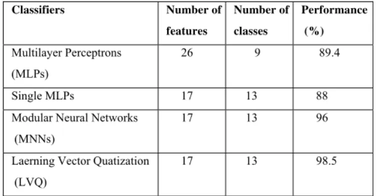
This paper addresses the issue of automating the classification tasks of wood defects. There has been a growing interest in research and development of automatic wood detection and classification techniques and systems, especially in wood-rich countries, such as Malaysia. Automated visual inspection systems with neural network classifiers have been widely applied to word defect classification [2]. Table 1 shows the classifiers used for wood defect using neural networks classifiers.
Table 1: Comparisons of different neural networks techniques for wood defect classification
Classifiers Number of
features
Number of
classes
Performance
(%)
Multilayer Perceptrons (MLPs)
26 9 89.4 Single MLPs 17 13 88 Modular Neural Networks
(MNNs)
17 13 96 Laerning Vector Quatization
(LVQ)
17 13 98.5
Pham and Sagiroglu [5] claimed that LVQ networks provide a high degree of discrimination between the different types of defects and potentially can perform defect classification in real time. These results together with other good reports on LVQ networks [6-7] have motivate the authors to applied S-LVQ networks for wood defect classification. In addition, S-LVQ networks have showed good classification performance for control chart pattern recognition [8].
II. SPIKINGNEURALNEYWORKS
This paper presents a more plausible network employing a Spiking Learning Vector Quantization (S-LVQ) network as pattern recognition. S-LVQ is usually trained by supervised learning vector quantization algorithm. In this network, instead of using the common neuron, spiking neurons are used as the processing elements. A spiking neuron is a simplified model of the biological neuron. It is, however, more realistic
A Computational Biological Network for Wood
Defect Classification
than the threshold gate used in perceptrons or sigmoidal gates (employed in MLPs). A clear justification of this is that, in a network of spiking neurons, the input, output, and internal representation of information, which is the relative timing of individual spikes, are more closely related to those of a biological network. This representation allows time to be used as a computational resource. It has been shown that networks of spiking neurons are computationally more powerful than these other neural network models [4]. However, spiking neural networks still lack good learning algorithms and architecture suitably simple for time series application such as control chart pattern recognition. As far as the author is concern, there is no application of spiking networks on wood defect classification. The aim of this work was to test whether S-LVQ networks could achieve good classification accuracy. The S-LVQ networks focus on the learning procedures and architecture of spiking neural networks for classifying wood defect.
The remainder of the paper is organized as follows. Section 2 describes the wood surface defect pattern recognition problem. Section 3 provides information on spiking neural network architecture. Section 4 describes the supervised S-LVQ Algorithm to train the network on wood veneer boards. Section 5 presents the results obtained and section6 discuss the paper.
III. WOODDEFECTCLASSIFICATIONPROBLEMS Fig.1 shows twelve common types of defects on wood veneer surfaces together with a photograph of defect free (clear) wood. Features were first extracted from different wood images containing known defect types or no defects. As in previous work [5], the classification experiments conducted in this work, the same 232 feature vectors representing clear wood and defective wood images were employed. Seventeen features were extracted from the wood images and used to train the S-LVQ classifier. The wood defect classification problem thus reduces to that of mapping a given set of seventeen features extracted from an image onto one of the image categories shown in Fig.1.
Fig 1: Categories of veneer wood images
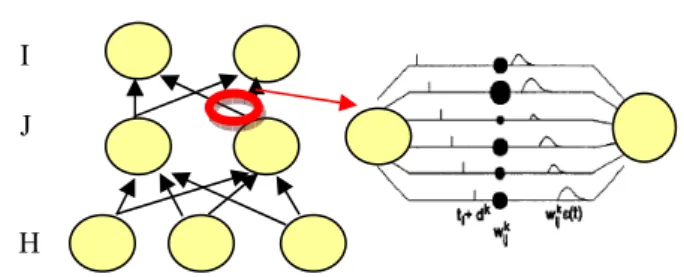
IV. ATYPICALSPIKINGNEURALNETWORKS Spiking neural networks have a similar architecture to traditional neural networks. Elements that differ in the architecture are the numbers of synaptic terminals between each layer of neurons and also the fact thatthere are synaptic delays. Several mathematical models have been proposed to describe the behaviour of spiking neurons, such as the Hodgkin-Huxley model [10], the Leakey Integrate-and-Fire model (LIFN) [11] and the Spike Response Model (SRM) [11]. Fig. 2 show the network structure as proposed by Natschlager and Ruf [13].
Fig 2: Feed forward spiking neural network
This structure consists of a feed forward fully connected spiking neural network with multiple delayed synaptic terminals. The different layers are labeled H, I, and J for the input, hidden, and output layer respectively as shown in Fig. 3. The adopted spiking neurons are based on the Spike Response Model to describe the relationship between input spikes and the internal state variable. Consider a neuron j , having a set Dj of immediate pre-synaptic neurons, receiving a
set of spikes with firing times ti , . It is assumed that any neuron can generate at most one spike during the simulation interval and discharges when the internal state variable reaches a threshold. The dynamics of the internal state variable are described by the following function:
(1)
Helpful
is the un-weighted contribution of a single synaptic terminal to the state variable which described a pre-synaptic spike at a synaptic terminal k as a PSP of standard height with delay .
(2)
The time is the firing time of pre-synaptic neuron i , and the delay associated with the synaptic terminal k. Considering the multiple synapses per connection case, the state variable of neuron j receiving input from all
Bark Clear wood
Colored streaks
Curly grain
Discoloration Holes Pin knots
Rotten knots
Roughness
Sound knots Split Streaks Worm holes
I J
neurons i is then described as the weighted sum of the pre-synaptic contributions as follows:
(3)
The effect of the input spikes is described by the function and so called the spike response function and is the weight describing the synaptic strengths. The spike response function , modelled with an -function, thus implementing a leaky- integrate-and fire spiking neuron, is given by:
(4)
is the time constant which defines the rise time and the decay time of the postsynaptic potential (PSP). The individual connection, which is described in [12], consists of a fixed number of m synaptic terminals. Each terminal serves as a sub-connection that is associated with a different delay and weight see Fig.3. The delay of a synaptic terminal k is defined as the difference between the firing time of the presynaptic neuron and the time when the postsynaptic potential starts rising. The threshold is a constant and is equal for all neurons in the network.
V. SPIKINGLEARNINGVECTORQUANTIZATION (S-LVQ)ARCHITECTUREINWOODCLASSIFICATION
A. Learning Vector Quantization (LVQ)
LVQ was developed by Kohonen [6]. This method has been implemented in an eponymous neural network.LVQ networks are simple, but accurate and fast classifiers [6-7]. They have been applied successfully to a variety of tasks in manufacturing engineering, including control chart pattern recognition [9] but so far only a few to the problem of wood defect classification. Fig. 3 shows an LVQ network comprising three layers of neurons: an input buffer layer, a hidden layer and an output layer. The network is fully connected between the input and hidden layers and partially connected between the hidden and output layers, with each output neuron linked to a different cluster of hidden neurons.
Fig 3: Standard learning vector quantization architecture
B. Proposed S-LVQ Architecture
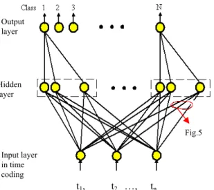
This paper proposes a new architecture for spiking neural networks for wood defect classification The proposed architecture consists of a feed forward network of spiking neurons which is fully connected between the input and hidden layers with multiple delayed synaptic terminals (m ) and partially connected between the hidden and output layers, with each output neuron linked to different hidden neurons. An individual connection consists of a fixed number of m synaptic terminals, where each terminal serves as a sub-connection that is associated with a different delay and weight between the input and hidden layers. The weights of the synaptic connections between the hidden and output neurons are fixed at 1. Experiments were carried out with a number of network structures with different parameters and learning procedures. The networks finally adopted had 17 input neurons in the input layer. One input neuron was therefore dedicated for each mean value. There were 13 output neurons, one for each defect category, and thirteen hidden neurons (the number of hidden neurons here depends on the number of classes). Table 2 show the configurations of the networks used.Fig.4 and 5 shows the structure of the networks and the multi-synapse connections respectively.
At the beginning of training, the synaptic weights were set randomly between 0 and +1. The input vector components were scaled between 0 and 1. Using a temporal coding scheme, the input vector components were then coded by a pattern of firing times within a coding interval and each input neuron allowed firing once at most during this interval.
Table 2: Details of the proposed S-LVQ network used for wood defect
Number of inputs = 17 Number of outputs = 13 Number of hidden neuron for each
output category = 13
Initial weights range = 0 to 1
Scaling range = 0 to 1 Coding interval = 0 to 100 Learning rate = 0.0075 Delay intervals = 15 (ms) in 10
(ms) interval
Synaptic delays = 1 to 16 (ms) Time constant = 120 (ms) Output
layer
Hidden layer
Input layer
Fig. 4: A structure proposed for the spiking neural network
Fig.5: Multi-synapse terminals for the spiking neural network In this work, the coding intervals T were set to [0-100] ms and the delays to {1,…,15} [ms] in 10 ms intervals. The available synaptic delays were therefore 1-16 ms. The PSP was defined by an function with a constant time =170 ms. Input vectors were presented sequentially to the network together with the corresponding output vectors identifying their categories as done in [2]. Unlike the network structure used in [11], the proposed structure helps to reduce the complexity of the connections where the multiple synaptic delays only exist between the input and hidden neurons. Only single connections between the hidden and output neurons and the weights were fixed to 1. This reduced the number of weights that had to be adjusted since only the connections between the input and hidden neurons had multiple synaptic terminals. The adopted spiking neurons were based on the Spike Response Model with some modification to the spike response function in order for the networks to be applied to wood veneer classification. The spike response function used in this architecture has been modified to:
(5) In this spike response function, tce and tci represent the maximum and minimum time constants respectively and tce=170 (ms) and tci=20 (ms). Here, st is equal to where t is the simulating time (0 to 300), is the firing time of presynaptic neurons and k d represents the delay with k =16. With this proposed spike response function, the spiking neural network technique worked well or at least at the standard level for wood defect classification.. Bohte et al [4] have stated that“Depending on the choice of suitable
spike response functions, one can adapt this model to reflect the dynamics of a large variety of different spiking neurons.”
C. S-LVQ Learning Procedures
In this work, a supervised learning equation was employed using the following update equations. If the winner is in the correct category, then:
(6)
(7)
(8) If the winner is in the incorrect category, then
(9)
(10) In the simulation, the parameter values for the learning function L ( ) were set to be:
= 0.0075, = 35, λ =
= [0-100], = 0.8, wnew is the new value for the weight
and wold is the old weight value. The parameter n is the
constant learning rate. Parameter sets the width of the positive part of the learning window and denotes the time difference between the onset of a PSP at a synaptic terminal and the time of the spike generated in the winning output neuron. Parameter was used because in supervised learning there is a priori information about the training sets. For this supervised learning procedure, the Winner-Takes-All learning rule modifies the weights between the input neurons and the neuron first to fire (winning neuron) in the hidden layer. The winner will be activated to 1 and the others to 0. In this learning procedure, only if the winning neuron is in the correct category and the start of the PSP at a synapse slightly precedes a spike in the target neuron, is the weight of this synapse increased, as it exerts a significant influence on the spike-time by virtue of a relatively large contribution to the membrane potential.
VI. CONCLUSION
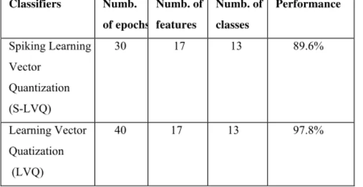
The results obtained with the proposed architecture and the supervised learning procedure for wood veneer classification are presented in Table 3 against the results reported previously with standard LVQ network [5].
Output layer
Hidden layer
Input layer in time coding
t1, t2, …, tn
Fig.5
Input vector,t
Table 3: Results comparing Standard LVQ and Spiking LVQ Classifiers Numb.
of epochs
Numb. of
features
Numb. of
classes
Performance
Spiking Learning Vector
Quantization (S-LVQ)
30 17 13 89.6%
Learning Vector Quatization (LVQ)
40 17 13 97.8%
Experiments yielded that S-LVQ with its simple configuration as showed in Table 2 give a standard level of performance for wood defect. As stated earlier, the spiking neural network still lack of good learning algorithm. So there are still a lot of research needs to be carried out in order to find the suitable one for an application. Although the performance accuracy is 89.6, the number of epochs it takes to achieve the accuracy is decrease These mean that the networks have the potential to perform defect classification in terms of better speeds of operation. This makes the S-LVQ system highly suitable for on-line real-time implementation in wood industries.
Previously, neural networks have proved capable of data smoothing and generalization. This paper has shown that spiking neural networks also have a good capability in data smoothing and generalization. This permits them to recognize noisy wood veneer defects and also other industrial automated inspection applications such quality control or specifically wood defect classification as indicated by the results presented in the paper
.
REFERENCES
[1] W. Polzleitner and G. Schwingshakl, “Real-time surface grading of profiled wooden boards,” Ind. Metrology, 1992, 2, 283-298.
[2] M.S. Packianather and P.R.Drake, “Comparison of Neural and Minimum Distance Classifiers in Wood Veneer Defect Identification,” IMechE Part B, J. of Engineering Manufacture, Vol.209, 2005, pp. 831-844.
[3] D.T. Pham and R.J. Alcock, “Automated visual inspection of wood boards:selection of features for defect classification by a neural network,” Proc. Instn Mech. Engrs, Part E, Journal of Process Mechanical Engineering, 1999, 213(E4), 231-245.
[4] M. Bohte, la Poutre H, J.N.Kok, “SpikeProp: ErrorBackpropagation for networks of spiking neurons,” ESANN 2000, Bruges (Belgium),pp 419-425.
[5] D T Pham and S Sagiroglu, “Neural Network Classification of Defects in Veneer Boards,” IMechE Part B, J. of Engineering Manufacture, Vol.214, 2000, pp. 255-258.
[6] T. Kohonen, “Self-Organisation and Associatives memory,3rd edition, “1989 (Springer-Verlag, Berlin). [7] D. Flotzinger, J. Kalcher and G. Pfurtscheller,
“LVQ-based on-line EEG classification,” In Proceedings of International Conference on Artificial Neural Networks and Genetic Algorithms, Innsbruck, Austria, 1993,pp 161-166.
[8] D.T. Pham and, S. Sahran, “Control chart pattern recognition using spiking neural networks,” Intelligent Production Machines and Systems 2nd I*PROMS Virtual International Conference, 3-14 July, 2006, pp 319-325. [9] D. T. Pham and E. Oztemel,”Control chart pattern
recognition using learning vector quantization networks,” Int. J. prod. Res, 1994, Vol 32, No. 3, pp 721-729.
[10] A. L.Hodgkin, A.F.Huxley, “A quantitative description of membrane current and its application to conduction and excitation in nerve,” Journal of Physiology. Vol. 117, No.4, 1952, pp. 500-544.
[11] W.Mass, “Networks of spiking neurons: the third generation of neural network models,”. Neural Networks,. Vol.10 , No.9, 1997, pp. 1659-1671.
[12] W. Bialek, F. Rieke, de Ruyter van Steveninck, R,D.Warland “Reading a neural code,” Science. Vol.252, No. 5014,1991, pp. 1854-1857.