Brazilian Journal of Physics, vol. 37, no. 2A, June, 2007 331
The van Hemmen Model in the Presence of a Random Field
Yamilles Nogueiraa, J. Roberto Vianaa, and J. Ricardo de Sousaa,b aDepartamento de F´ısica, Universidade Federal do Amazonas
3000, Japiim, 69077-000, Manaus-AM, Brazil
b Departamento de F´ısica, ICEx,
Universidade Federal de Minas Gerais, Av. Antˆonio Carlos 6627, CP 702, 30123-970, Belo Horizonte-MG, Brazil
Received on 12 July, 2006
The van Hemmen model with a random field is studied to analyze the tricritical behavior in the Ising spin
glass phase. The free energy and phase diagram (T versusH andT versusJo/J, whereHis the root mean
square deviation of the magnetic field,JoandJare the ferromagnetic and root mean square deviation exchange,
respectively) are calculated for the model with discrete (or bimodal) and Gaussian distributions. For the case of the bimodal probability distribution (random field and exchange), we have the presence of three ordered phases,
namely: spin glass (SG), mixed (∏) and ferromagnetic (F). The root mean square deviation of the random field
Hdestroys the spin glass and mixed phases. The mixed phase doesn’t appear with Gaussian distribution. In the
planeTversusH, we analyze the tricritical behavior for the case of the bimodal distribution, and we compare it
with the results obtained by using the Gaussian distribution that presents only second-order phase transition.
Keywords: Spin glasses; Random fields; van Hemmen model; Tricritical behavior
I. INTRODUCTION
The study of the random field Ising model (RFIM) has been a topic of great interest in recent years because of its physical realization as a diluted Ising antiferromagnet in the presence of a uniform magnetic field along the uniaxial direction [1]. The lower critical dimension of the RFIM, above which there exists a stable ferromagnetic state at low temperatures, has been suggested by Imry and Ma [2] that is dl =2. Using mean field approximation, the nature of the phase transition depends on the distribution associated with the magnetic field. For the Gaussian distribution, the phase transition is always continuous [3], and with symmetric bimodal distribution the phase transition is continuous in the region of low and high temperature, becoming first order for sufficiently large values of magnetic field (random) and low temperature[4]. Study of the three-dimensional RFIM using Monte Carlo simulation detects a jump in the magnetization but no latent heat for both bimodal [5] and Gaussian[6] distributions. However, in four dimensions a zero temperature scaling analysis [7] leads to a first-order phase transition in the bimodal case and a contin-uous one for a Gaussian distribution, which is in agreement with the mean-field predictions. The use of the mean-field approximation at zero temperature has shown that the order parameter exponent (β) varies continuously with the disorder, under the power law distribution of random field [8], i.e., non-universal behavior.
The diluted antiferromagnet FexZn1−xF2, due to large crystal-field anisotropy, when submitted to an external uni-form magnetic field become good experimental realization of the RFIM [9] for large enough values of the concentrationx. Asxdecreases, they behave like Ising spin glass. The spin glass theory has been a difficult problem in statistical me-chanics [10]. For many years there has been great contro-versy on whether the spin glass transition is either of
ther-modynamical or of dynamic nature. A number of physical examples exist. The canonical cases are the metallic alloys with substitutional magnetic impurities, such as CuMn and AuFe. A necessary requirement sums to be a locally random competition between ferromagnetic and antiferromagnetic in-teractions. However this competition may have a number of possible microscopic states, for example, fixed positions but random exchange, fixed exchange interaction as a function of distance but random positions (RKKY interaction), etc.
Recently, the Ising spin glass with random field in the ver-sion of the model proposed by Sherrington and Kirkpatrick (SK) [11] has been treated for Gaussian [12] and bimodal [13] distributions (characterized by a mean valuehHii=0 and the root mean square deviationH=q
Hi2® ). The joint study of spin glass and random field problems has been proposed as an appropriate system for the description of mixed hydrogen-bonded ferroelectrics and antiferroelectrics, the so-called pro-ton and deuteron glasses [14, 15], which may be considered as the electric counterparts of magnetic spin glass. On the experimental front, certain classes of randomly dilute antifer-romagnets [9], the phase separation of binary fluids in porous media [16]-[18] and the liquid-vapor critical point in porous media[19] are also all believed to be realizations of the RFIM. Experimental works in the FexZn1−xF2compound suggest that forx≥0.40 one gets a RFIM, whereas forx≤xp=0.24 (percolation concentration) it becomes an Ising spin glass (ISG). On the other hand, for intermediate concentrations (0.25≤x≤0.40) a crossover between the RFIM and ISG for small and large magnetic fields, respectively is clearly ob-served in measurements of Fe0.31Zn0.69F2[20]-[22].
332 Yamilles Nogueira et al.
does not require the use of the replica trick. In spite of being non-realistic, mean field models give a first qualitative under-standing of the thermodynamic behavior. Among these are the susceptibility cusp at the freezing temperatureTf and the field-induced transition away from the spin glass phase at fi-nite magnetic field. Recently, the quantum version (presence of a transverse magnetic field) [24] and an additional multi-spin interactions [25] in the van Hemmen model have been treated in the literature.
The outline of the remainder of the paper is as follows: In Section 2, we introduce the model, where obtain an analytical expression for the free-energy and equations of state. In Sec-tion 3, we exhibit and discuss the phase diagrams. Finally, in Section 4 we present our conclusions.
II. MODEL AND FORMALISM
To treat the influence of the random field in the spin glass phase, we generalize the van Hemmen model of spin glass, that consists of a fully connected lattice ofNIsing spins with a random field described by the following Hamiltonian:
H
=−Jo N(∑
i,j)
Si.Sj−
∑
(i,j)
Ji jSi.Sj−
∑
iHiSi, (1)
where (i,j) denotes a sum over all possible pairs of spins, Jo represents a ferromagnetic interaction, Hi is the random field,Si=±1 is the spin variable at sitei,Ji jis the spin glass random coupling given by
Ji j= J
N(ξiηj+ξjηi), (2) where theξi’s,ηi’s andHiare independent, identically distrib-uted random variables with even distribution around zero and a finite variance.
In the model (1), the ferromagnetic bonds (Jo) favour a par-allel alignment of the spins whereas antiferromagnetic bonds (random exchangeJi j) favour an antiparallel alignment. The competition of ferromagnetic and antiferromagnetic bonds in-ducefrustration, ingredient to a spin glass model. In
particu-lar, we restrict ourselves to the cases the two different distrib-utions: discrete (or bimodal distribution) given by
P
(xi) =12[δ(xi−σxi) +δ(xi+σxi)], (3)
and the Gaussian (continuous distribution)
P
(xi) = 1 q2πσ2 xi
exp£−x2i/(2σ2 xi)
¤
, (4)
wherexi≡ξi, ηi,Hi,σξ =ση =1 and σH =
q
Hi2®≡H. The parametersH andJare the square-root deviation of the probability distribution associated with the random magnetic field and exchange couplings, respectively.
In the thermodynamic limitN→∞, the van Hemmen model has three order parameters [23]
m= lim N→∞
( 1 N
N
∑
i=1
hSii )
, (5)
q1= lim N→∞
( 1 N
N
∑
i=1
hξiSii )
, (6)
and
q2= lim N→∞
( 1 N
N
∑
i=1
hηiSii )
, (7)
which have to be chosen in such a way that−→M = (m,q1,q2) minimizes a certain free-energy functional. The number of independent random variables is 2N in contrast with N22 of SK model. Thus we have a random-site problem and not a random-bond problem as in most other SG models, in agree-ment with the experiagree-mental situation.
The second term of the Hamiltonian (1) can be separable, i.e.,
∑
i6=j
(ξiηj+ξjηi)SiSj= "
N
∑
i=1
((ηi+ξi)Si) #2
−
à N
∑
i=1
ηiSi !2
−
à N
∑
i=1
ξiSi !2
−2
∑
iξiηi, (8)
so that the Eq. (1) can be rewritten as
H
= −Jo N(∑
i,j)
Si.Sj− J N
"
N
∑
i=1
((ηi+ξi)Si) #2
−
à N
∑
i=1
ηiSi !2
−
à N
∑
i=1
ξiSi !2
+2J
N
∑
i ξiηi−∑
i HiSi, (1)Brazilian Journal of Physics, vol. 37, no. 2A, June, 2007 333
1.6 2.0 2.4
0.0 0.2 0.4 0.6 0.8 1.0 (d) F P T/J
J0/J
0.0 0.4 0.8 1.2 1.6 2.0 2.4 2.8
0.0 0.2 0.4 0.6 0.8 1.0
0.0 0.2 0.4 0.6 0.8 1.0 1.2 1.4 0.0 0.2 0.4 0.6 0.8 1.0 1.2 1.4 T/J
J0/J F P
SG
(c)
0.0 0.2 0.4 0.6 0.8 1.0 1.2 1.4
0.0 0.2 0.4 0.6 0.8 1.0 1.2 1.4
0.0 0.2 0.4 0.6 0.8 1.0 1.2 1.4 0.0 0.2 0.4 0.6 0.8 1.0 1.2 1.4 (b) F SG P T/J
J0/J
0.0 0.2 0.4 0.6 0.8 1.0 1.2 1.4
0.0 0.2 0.4 0.6 0.8 1.0 1.2 1.4
0.0 0.2 0.4 0.6 0.8 1.0 1.2 1.4 0.0 0.2 0.4 0.6 0.8 1.0 1.2 1.4 (a) 3 T/J
J0/J
SG F
P
0.0 0.2 0.4 0.6 0.8 1.0 1.2 1.4
0.0 0.2 0.4 0.6 0.8 1.0 1.2 1.4
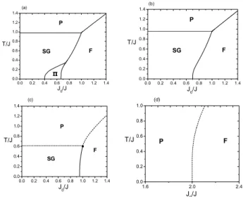
FIG. 1: Phase diagram in the planeT/JversusJo/Jfor the van
Hem-men spin glass model with a symmetricbimodalrandom field and
various magnitude ofδ=H/J. The full and dashed lines represent
second-order (continuous) and first-order phase transitions,
respec-tively. The ferromagnetic (F), spin glass (SG) and mixed (∏) critical
frontiers change qualitatively for increasing values ofδ. (a)δ=0.10;
(b)δ=0.20; (c)δ=0.45; (d)δ=1.0.
have to calculate the partition function
Z=Tr{exp(−β
H
)}=∑
µ
µ¯¯exp(−β
H
) ¯¯µ®, (10)
for the ortogonal complete set of states|µi, where we use the Gaussian identity
exp(αx2) =√1 2π
∞ Z
−∞
dyexp(−y
2
2 +
√
2αxy) (11)
Performing the trace and using steepest descent integra-tions, we obtain, after some algebra, the following expression for the free-energy per spin
βf(m,q) =β 2(Jom
2+2Jq2)− hln[2 cosh(βW)]i
c, (12) whose minimum corresponds always toq1=q2=qand the equations of states are given by
m=
ZZZ
P
(ξ)P
(η)P
(Hi)dξdηdHitanh(βW) (13)and
q=
ZZZ
P
(ξ)P
(η)P
(Hi)dξdηdHi(η+ξ)
2 tanh(βW), (14) whereW =Hi+Jom+Jq(ξ+η)and the notationh....ic de-note the average over the random variableη,ξandHi.
III. RESULTS AND DISCUSSION
In the limit of null random field, the above equations reduce to the same expressions obtained by van Hemmen [23]. The
0.8 1.2 1.6 2.0 0.0 0.2 0.4 0.6 0.8 1.0 T/J
J0/J
0.0 0.4 0.8 1.2 1.6 2.0 2.4 2.8
0.0 0.2 0.4 0.6 0.8 1.0 (c) P F
0.0 0.2 0.4 0.6 0.8 1.0 1.2 1.4 0.0 0.2 0.4 0.6 0.8 1.0 1.2 1.4 T/J
J0/J
0.0 0.2 0.4 0.6 0.8 1.0 1.2 1.4
0.0 0.2 0.4 0.6 0.8 1.0 1.2 1.4 (b) SG F P
0.0 0.2 0.4 0.6 0.8 1.0 1.2 1.4 0.0 0.2 0.4 0.6 0.8 1.0 1.2 1.4 T/J
J0/J
0.0 0.2 0.4 0.6 0.8 1.0 1.2 1.4
0.0 0.2 0.4 0.6 0.8 1.0 1.2 1.4 (a) P F SG
FIG. 2: Phase diagram in the planeT/J versus Jo/J for the van
Hemmen spin glass model with aGaussianrandom field and
var-ious magnitude ofδ=H/J. The ferromagnetic (F) and spin glass
(SG) critical frontiers change qualitatively for increasing values ofδ:
(a)δ=0.20; (b)δ=0.45; (c)δ=1.0.
phase diagram in the (T/J,α) plane, whereα=Jo/Jand the Boltzmann constantkB=1, presents three ordered phases: i)
Ferromagnetic-F; ii)Spin Glass-SG andMixed-∏ phases.
The mixed phase doesn’t appear for the case of the Gaussian distribution. The F, SG and
∏
phases are determined by means of two order parameter,mandqwhich are the magneti-zation and the spin-glass order parameter, respectively. When m and q are nonzero, we have the∏
phase. The F and SG phases are characterized by (m6=0,q=0) and (m=0,q6=0), respectively. A stable phase (m,q) corresponds to a global maximum of the free energy functional, Eq. (12), whereas a metastable phase gives rise to a global maximum.In Fig. 1, we present the phase diagram in the (T/J, α) plane for some values ofδ=H/Jwithbimodal distribution. We also have the paramagnetic phase (P) corresponding to the trivial solutionm=q=0. The critical frontiers (F-SG, F-∏, SG-P, SG-∏and F-P) are obtained numerically from Eq.(12) equaling the free energies by imposing the conditions for the mandq parameters in the respective phases (F,∏, SG, P), and also using Eqs. (13) and (14). It can be seen that the effect of the random field is to destroy the SG and∏ordered phases (Fig. 1a). Forδ>δ1c=0.17 the mixed phase (∏) disappears (see Fig. 1b). An interesting behavior is observed for small range of field magnitudes, that for 0.44<δ<0.50 one observes a first-order phase transition in the SG-P and F-P critical frontiers, while in the case of the F-SG critical frontier, we don’t have latent heat, i.e., the phase transition is of second-order (Fig. 1c). Forδ>δ2c=0.5, the SG phase is destroyed and only the F phase is present in the phase diagram with a phase transition of first-order (Fig. 1d).
334 Yamilles Nogueira et al.
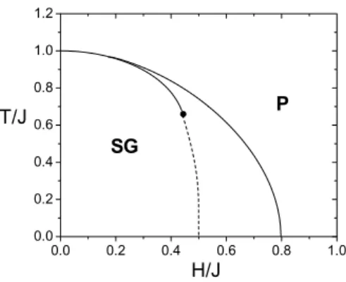
0.0 0.2 0.4 0.6 0.8 1.0
0.0 0.2 0.4 0.6 0.8 1.0 1.2
P
SG
H/J T/J
0.0 0.2 0.4 0.6 0.8 1.0
0.0 0.2 0.4 0.6 0.8 1.0 1.2
FIG. 3: Phase diagram in the planeT/JversusH/Jfor the van
Hem-men spin glass model with bimodal and Gaussian random field for
α=0.
H/Jwith Gaussian distribution is presented. We have found analytically a critical fieldδc=
q
2
π ≃0.80, where for δ>
δc the SG phase is destroyed and the F phase exists for all value of finite random field, F-P critical line being the a phase transition of second-order.
In Fig. 3, we present in the planeT/Jversusδthe behav-ior of the critical temperature for the SG-P phase transition for the cases of bimodal and Gaussian distributions. The most interesting effect exhibited in Fig. 3 is the presence of a tricrit-ical point (TCP) in the VH model when the random field de-scribed by bimodal distribution. In the null temperature limit we obtainδ2c=0.50 that separates the SG and P phases by a phase transition of first-order. On the other hand, for the case of Gaussian distribution we found the value of the
criti-cal fieldδc= q
2
π≃0.80 where the temperature goes to zero with a second-order phase transition.
IV. CONCLUSIONS
In conclusion, we have studied the van Hemmen spin glass model in the presence of a random field. We have analyzed the phase diagram for the cases of bimodal and Gaussian distributions in the random field. For the case of the bimodal distribution we observe three ordered phases, namely: F (ferromagnetic), SG (spin glass) and∏(mixed). The mixed phase does not appear with Gaussian distribution. We have shown that for δ >δ1c=0.17 the mixed phase disappear, while the SG phase gets destroyed (disappear) at δ>0.50 for the bimodal distribution and atδ>q2
π≃0.80 for the Gaussian distribution. Only the F-P phase transition is present all through. We have observed first-order phase transition between the SG-P and F-P phase transitions for the case of the bimodal distribution in small range of field magnitude 0.44 < δ < 0.50. For the same probability distribution at δ>0.50 the SG phase is destroyed and the F-P phase transition is of first-order. On the other hand, in the case of Gaussian distribution the phase transitions are all of second-order.
Acknowledgments
We are grateful to Dr. Puspitapallab for helpful discussions. The work was financial supported by CNPq, FAPEAM and CAPES (Brazilian agencies).
[1] S. Fishman and A. Aharony, J. Phys. C12, L729 (1979).
[2] Y. Imry and S. K. Ma, Phys. Rev. Lett.35, 1399 (1975).
[3] T. Schneider and E. Pytte, Phys. Rev. B15, 1519 (1977).
[4] A. Aharony, Phys. Rev. B18, 3318 (1978).
[5] H. Rieger and A. P. Young, J. Phys. A26, 5279 (1993).
[6] H. Rieger, Phys. Rev. B18, 6659 (1995).
[7] M. R. Swift, A. J. Bray, A. Maritan, M. Cieplak, and J. R.
Ba-navar, Europhys. Lett.38, 273 (1997).
[8] R. Dobrin, J. H. Meinke, and P. M. Duxbury, J. Phys. A35,
L247 (2002).
[9] D. Belanger,Spin Glass and Random Fields, edited by A. P.
Young (World Scientific, Singapore, 1997).
[10] K. Binder and A. P. Young, Rev. Mod. Phys.58, 801 (1986).
[11] D. Sherrington and S. Kirkpatrick, Phys. Rev. Lett.35, 1792
(1975).
[12] R. F. Soares, F. D. Nobre, and J. R. L de Almeida, Phys. Rev.
B50, 6151 (1994).
[13] E. Nogueira Jr., F. D. Nobre, F. A. da Costa, and S. Coutinho,
Phys. Rev. E57, 5079 (1998).
[14] R. Pirc, B. Blinc, and W. Wiotte, Physica B182, 137 (1992).
[15] R. Pirc, B. Taic, and R. Blinc, Physica A185, 322 (1992).
[16] J. V. Maher, W. I. Goldburg, D. W. Pohl, and M. Lanz, Phys.
Rev. Lett.53, 60 (1984).
[17] M. C. Goh, W. I. Goldburg, and C. M. Knobler, Phys. Rev. Lett.
58, 1008 (1987).
[18] P. Wiltzius, S. B. Dierker, and B. S. Dennis, Phys. Rev. Lett.
62, 804 (1989).
[19] A. Wong and M. H. W. Chan, Phys. Rev. Lett.65, 2567 (1990).
[20] F. C. Montenegro, A. R. King, V. Jaccarino, S. -J. Han, and D.
P. Belanger, Phys. Rev. B44, 2155 (1991).
[21] D. P. Belanger, Wm. E. Murray Jr., F. C. Montenegro, A. R.
King, V. Jaccarino, and R. W. Erwin, Phys. Rev. B44, 2161
(1991).
[22] S. M. Rezende, F. C. Montenegro, U. A. Leit˜ao, and M. D.
Coutinho-Filho, inNew Trends in Magnetism, edited by M. D.
Coutinho-Filho and S. M. Rezende (World Scientific, Singa-pore, 1998).
[23] J. L. van Hemmen, Phys. Rev. Lett.49, 409 (1982).
[24] J. Roberto Viana, Yamilles Nogueira, and J. Ricardo de Sousa,
Phys. Rev. B66, 113307 (2002); ibid Phys. Lett. A311, 480
(2003).
[25] P. T. Muzy, A. P. Vieira, and S. R. Salinas, Physica A359, 469