Generalized Exponential Distribution in Flood Frequency Analysis for Polish Rivers.

Generalized Exponential Distribution in Flood

Frequency Analysis for Polish Rivers

Iwona Markiewicz1

*, Witold G. Strupczewski1_{, Ewa Bogdanowicz}2_{, Krzysztof Kochanek}1

1Department of Hydrology and Hydrodynamics, Institute of Geophysics Polish Academy of Sciences, Warsaw, Poland,2CHIHE Norway Grants, Institute of Geophysics Polish Academy of Sciences, Warsaw, Poland

*iwonamar@igf.edu.pl

Abstract

Many distributions have been used in flood frequency analysis (FFA) for fitting the flood extremes data. However, as shown in the paper, the scatter of Polish data plotted on the moment ratio diagram shows that there is still room for a new model. In the paper, we study the usefulness of the generalized exponential (GE) distribution in flood frequency analysis for Polish Rivers. We investigate the fit of GE distribution to the Polish data of the maximum flows in comparison with the inverse Gaussian (IG) distribution, which in our previous stud-ies showed the best fitting among several models commonly used in FFA. Since the use of a discrimination procedure without the knowledge of its performance for the considered probability density functions may lead to erroneous conclusions, we compare the probability of correct selection for the GE and IG distributions along with the analysis of the asymptotic model error in respect to the upper quantile values. As an application, both GE and IG distri-butions are alternatively assumed for describing the annual peak flows for several gauging stations of Polish Rivers. To find the best fitting model, four discrimination procedures are used. In turn, they are based on the maximized logarithm of the likelihood function (K proce-dure), on the density function of the scale transformation maximal invariant (QKprocedure), on the Kolmogorov-Smirnov statistics (KSprocedure) and the fourth procedure based on the differences between the ML estimate of 1% quantile and its value assessed by the method of moments and linear moments, in sequence (Rprocedure). Due to the uncertainty of choosing the best model, the method of aggregation is applied to estimate of the maxi-mum flow quantiles.

Introduction

Flood frequency analysis (FFA) provides information about the probable size of flood flows and has been used for the design of civil engineering works over the century. The assessment of the flood (upper) quantiles is required for dimensioning hydraulic structures affected by high waters, such as culverts, dams, bridges, overflow channels, spillways, levees, and others. FFA plays an important role in reducing the flood risk, since the flood quantile estimates are essen-tial in determining the limits of flood zones with varying degree of flood risk as well in estimat-ing the risk of exploitation of floodplains.

OPEN ACCESS

Citation:Markiewicz I, Strupczewski WG, Bogdanowicz E, Kochanek K (2015) Generalized Exponential Distribution in Flood Frequency Analysis for Polish Rivers. PLoS ONE 10(12): e0143965. doi:10.1371/journal.pone.0143965

Editor:Xi Luo, Brown University, UNITED STATES

Received:April 22, 2015

Accepted:November 11, 2015

Published:December 10, 2015

Copyright:© 2015 Markiewicz et al. This is an open access article distributed under the terms of the Creative Commons Attribution License, which permits unrestricted use, distribution, and reproduction in any medium, provided the original author and source are credited.

Data Availability Statement:The data of the annual maximum flow series for selected gauging stations of Polish Rivers have been bought from the Institute of Meteorology and Water Management in Warsaw, Poland, and the authors are obligated not to publish them. Interested researchers can purchase these data by contacting The Expertise Department (historical data) atekspertyzy@imgw.pl, +48 22 56 94 381 or +48 22 56 94 254. However, the statistical characteristic of these series and other relevant data are within the paper.

The quantile of the order ofF2(0,1) is defined as the valuexFsatisfying the equation:

Z xF

1

fðxÞdx¼F ð1Þ

wherefis the probability density function (PDF) of the continuous random variable. Theflood (upper) quantile means the probable maximumflow of the return period ofTyears and the relation between the probability of non-exceedanceFand return periodThas the form:

T¼₁ 1

F ð2Þ

Since the return periodTequal to 100, 500, 1000 is usually used, then the probabilityFis close to 1, i.e. close to its highest value. Equivalently, the probabilities of exceedancepcan be applied, where:

p¼1 _{F ð3Þ}

The at-site frequency analysis is the most commonly used approach. Then the estimation of flood quantiles refers to the choice of the form of probability density function describing the annual peak flows for the investigated gauging station. The distribution function assumed (also called the model) has a character of statistical hypothesis. Simultaneously, the method of esti-mation of parameters and, thus, upper quantiles of the assumed distribution is selected. This step is denoted D/E for“distribution and estimation procedure”. To find the best fitting model to the empirical data, the chosen discrimination procedure is applied.

The choice of distribution for fitting the annual maximum flows has attracted considerable interest, e.g. [1–7] and many others. According to the hydrological report of the World Meteo-rological Organization from 1989 [8], the Gumbel and log-normal distributions were the most commonly used for the description of the peak flow data. In Poland, the Pearson III type distri-bution has been recommended by Central Office of Water Management for national use [9]. These regulations are still in force, although other models are also applied in practice. Nowa-days in many countries around the world, the heavy-tailed distributions are recommend for modelling of extreme flow series, e.g. [10–15]. The heavy-tailed distributions have conventional moments only in a certain range, which decreases with growing moment order. However, the heavy-tailed form of hydrological variables is not sufficiently supported, e.g. [16], [17]. More-over, the analysis of Polish datasets of annual peak flows in [18] shows that they should be modeled using soft-tailed rather than heavy-tailed distributions.

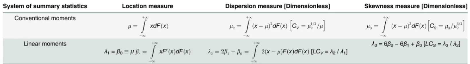
The characteristics describing properties of the distribution are the summary statistics. Sev-eral systems of summary statistics have been developed. Based on different principles they pro-vide, in particular, the measures of location, dispersion, skewness and kurtosis. The summary statistics calculated for a random sample consecutively serve for identifying and fitting PDFs. Among the systems of summary statistics, the most popular are the system of conventional moments (μr) and that of linear moments, calledL-moments (λr), presented inTable 1along

with the dimensionless versions of the summary statistic sets in the form of summary statistic

Table 1. Summary statistics according to the system of conventional and linear moments.

System of summary statistics Location measure Dispersion measure [Dimensionless] Skewness measure [Dimensionless]

Conventional moments

m¼ Zþ1

1

xdF xð Þ m2¼

Zþ1

1 ðx mÞ2

dFðxÞ CV¼m

1=2 2 =m

h i

m3¼ Zþ1

1 ðx mÞ3

dFðxÞCS¼m3=m 3=2 2

h i

Linear moments

λ1=β0μbr¼

Zþ1

1

xFr

ðxÞdFðxÞ l2¼2b1 b0¼ Zþ1

1

2_ðx mÞFðxÞdFðxÞ[LCV=λ2/λ1]

λ3= 6β2−6β1+β0[LCS=λ3/λ2] features of flood waves“, decision nr DEC-2012/05/B/

ST10/00482 and by the Polish Ministry of Science and Higher Education under the Grant Iuventus Plus IP 2010 024570 titled“Analysis of the efficiency of estimation methods in flood frequency modelling”. This work was partially supported within statutory activities No 3841/E-41/S/2015 of the Ministry of Science and Higher Education of Poland.

ratios (in square brackets). It is convenient to use the dimensionless versions of the summary statistics, since they measure the shape of a distribution independently of its scale of

measurement.

As seen fromTable 1, theL-moments can be defined by the probability weighted moments of a random variableβ_rforr= 0,1,2,. . ._{[19]. TheL-moments create an attractive system} because their estimators, in contrast to the classical moments estimators, are not biased and the samplingL-moment ratios have very small biases for moderate and large samples.

For the convenience of the reader, the abbreviations and symbols commonly used in the paper are gathered in Table inS1 Table.

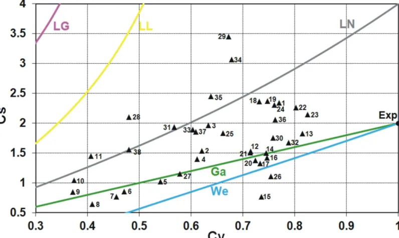
For two-parameter distributions lower bounded at zero, a basic illustration that provides an intuition to a practitioner to distinguish various distributions is the graph of the relationship between the conventional variation coefficientCVand the conventional skewness coefficientCS

or between their linear counterparts, i.e. between the linear variation coefficientLCVand the

linear skewness coefficientLCS. These relationships show in what range ofCV−CSvarious

dis-tributions can be used, e.g. the log-logistic and log-Gumbel disdis-tributions are not proper for modelling the data series of small skewnessCS<1 and average variationCV>0.5.Both

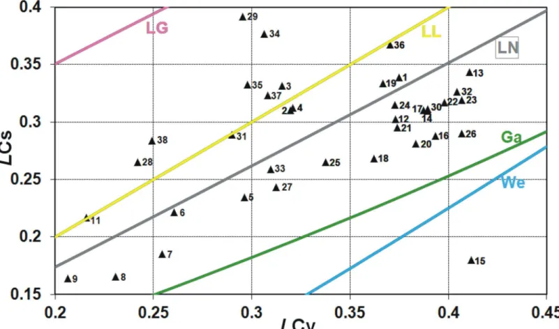
rela-tions,CV−CSandLCV−LCS, are shown in Figs1and2, respectively, for two-parameter

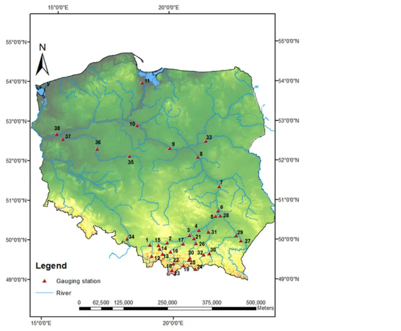
distri-butions commonly used in FFA (lines) plotted with the Polish data of annual peak flows for 38 gauging stations (triangular points). To find the data availability, see the Acknowledgment.

Fig 1. The relation of conventional skewness coefficientCSversus conventional variation coefficientCVfor some two-parameter distributions

commonly used if FFA plotted with the Polish data of 90-year annual peak flow series.Distributions: Ga–gamma, We–Weibull, LN–log-normal, LL–

log-logistic, LG–log-Gumbel, Exp–exponential.

In Figs1and2, if some point lies on the line corresponding to certain distribution or around it, it may indicate that this distribution will be the best fitting to the data series. However, the perfect fit would hold for the asymptotic sample from a given distribution. Due to a limited length of the data series, such graphical analysis is only preliminary and the distribution best fitted to the data is indicated by the discrimination procedures, which will be discussed later in this paper.

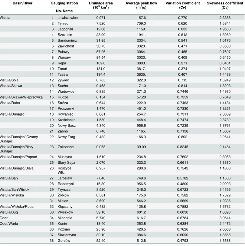
The respective measuring sections are listed inTable 2and illustrated inFig 3. Most of ana-lyzed data series cover the period 1921–2010.

As seen in Figs1and2, for both conventional and linear moments ratios, there is a range of values taken by the Polish data series and not covered by any distribution. Clearly, there is still room for a new model. The inverse Gaussian (IG) and the generalized exponential (GE) distri-butions with the scale and shape parameters seem to be a suitable complement (see Figs4and

5), i.e. there are many pointsCV-CScorresponding to the Polish data series, which are on or

around the lines of IG and GE distributions.

The GE distribution is used quite effectively to analyze lifetime data in the reliability analy-sis, being an alternative to the two-parameter gamma, Weibull, Pareto and log-normal distri-butions [20]. The aim of the study is to assess the usefulness of the generalized exponential distribution in flood frequency analysis for Polish Rivers, as a complementary to the inverse Gaussian distribution, which has proved to be suitable for many Polish data series [21], [22],

Fig 2. The relation of linear skewness coefficientLCSversus linear variation coefficientLCVfor some two-parameter distributions commonly used

if FFA plotted with the Polish data of 90-year annual peak flow series.Distributions: Ga–gamma, We–Weibull, LN–log-normal, LL–log-logistic, LG–

log-Gumbel, Exp–exponential.

[18]. In the paper, two-parameter distributions, instead of their three-parameter counterparts, are used for the modelling of relatively large-size samples (i.e. 90 elements), since our studies are intended to be applicable for most of the available observation series, which are much shorter than those investigated here. The short length of the data series hinders the proper

Table 2. Origin and basic characteristics of 38 Polish gauging stations.

Basin/River Gauging station Drainage area (103km2)

Average peakflow (m3/s)

Variation coefficient (Cv)

Skewness coefficient (CS)

No. Name

Vistula 1 Jawiszowice 0.971 157.6 0.770 2.3388

2 Tyniec 7.520 709.0 0.620 1.5344

3 Jagodniki 12.06 1159. 0.633 1.9630

4 Szczucin 23.90 1941. 0.612 1.3989

5 Sandomierz 31.85 2334. 0.541 1.0175

6 Zawichost 50.73 3328. 0.471 0.8530

7 Puł_{awy 57.26 3064. 0.455 0.7697}

8 Warsaw 84.54 3023. 0.409 0.6450

9 Kępa 169.0 3803. 0.371 0.8461

10 Toruń 181.0 3817. 0.374 1.0407

11 Tczew 194.4 3635. 0.407 1.4483

Vistula/Sola 12 Żywiec 0.785 322.8 0.715 1.5249

Vistula/Skawa 13 Sucha 0.468 171.0 0.814 1.8293

14 Wadowice 0.835 271.3 0.7446 1.4980

Vistula/Skawa/Wieprzówka 15 Rudze 0.154 57.28 0.7359 0.7649

Vistula/Raba 16 Stróża 0.644 222.9 0.7463 1.4184

17 Proszówki 1.470 451.0 0.7330 1.3251

Vistula/Dunajec 18 Kowaniec 0.681 254.7 0.7311 2.3639

19 Krościenko 1.580 448.4 0.7474 2.3732

20 Nowy Sącz 4.340 956.6 0.7239 1.3761

21 Żabno 6.740 1165. 0.7138 1.5067

Vistula/Dunajec/ Czarny Dunajec

22 Nowy Targ 0.432 166.3 0.802 2.2641

Vistula/Dunajec/Biał_y Dunajec

23 Zakopane 0.058 39.09 0.8245 2.1484

Vistula/Dunajec/Poprad 24 Muszyna 1.510 234.8 0.7602 2.3053

25 Stary Sącz 2.070 323.2 0.6611 1.8310

Vistula/Dunajec/Biał_{a 26 Koszyce} Wlk.

0.957 280.6 0.7543 1.1083

Vistula/San 27 Jarosł_{aw 7.040 749.6 0.5782 1.1508}

28 Radomyśl 16.80 956.5 0.4800 2.0993

Vistula/San/Wisł_{ok 29 Tryńcza 3.520 246.3 0.6723 3.4536}

Vistula/Wisł_{oka 30 Żó}ł_{ków 0.581 175.6 0.7582 1.7529}

31 Mielec 3.690 546.2 0.5669 1.9336

Vistula/Wisłoka/Ropa 32 Klęczany 0.482 125.8 0.7882 1.6732

Vistula/Bug 33 Wyszków 39.10 601.2 0.6030 1.8896

Oder 34 Miedonia 6.740 616.7 0.6784 3.0644

Oder/Warta 35 Konin 13.40 252.8 0.6384 2.4472

36 Poznań 25.90 420.5 0.7626 2.0603

37 Skwierzyna 32.10 384.6 0.6090 1.8565

38 Gorzów 52.40 512.8 0.4793 1.5588

selection of the distribution and two-parameter PDFs are usually used for their modelling. To reduce the uncertainty in the estimation of the extreme value distribution quantiles, the multi-model approach proposed by Bogdanowicz [23] is applied.

The paper is organized as follows. After providing some introduction to the topic, the prob-ability distributions analyzed in the paper are shortly presented in second section. Next, the four discrimination procedures used to select the best fitting model are shown. Sequent two sections provide the results of the simulation studies on the probability of correct selection (PCS) among the GE and IG distributions along with the analysis of the asymptotic model error in respect to the upper quantile. In the case study section, fitting the GE and IG distribu-tions to the 90-year series of annual maximum flows is compared for four selected gauging sta-tions of Polish Rivers. Then, the method of aggregated quantiles is proposed for evaluation of upper quantile values. The paper is concluded in the final section.

Fig 3. Map of 38 Polish gauging stations.

GE and IG Probability Distributions

The inverse Gaussian (known also under the name of Wald) distribution has several properties analogous to the Gaussian distribution. In fact, the name is misleading, since it is“inverse” only in that, while the Gaussian describes the distribution of distance at a fixed time in

Fig 4. The relation of conventional skewness coefficientCSversus conventional variation coefficientCVfor two-parameter inverse Gaussian, IG,

and generalized exponential, GE, distributions plotted with the Polish data of 90-year annual peak flow series.

doi:10.1371/journal.pone.0143965.g004

Fig 5. The relation of linear skewness coefficientLCSversus linear variation coefficientLCVfor two-parameter inverse Gaussian, IG, and

generalized exponential, GE, distributions plotted with the Polish data of 90-year annual peak flow series.

Brownian motion, the inverse Gaussian describes PDF of the first passage time for a Brownian motion starting at zero to reach the absorbing barrier at the fixed point [24]. The same function appears in linear flood routing modelling as the impulse response of the semi-infinite channel at a fixed distance for the Froude number equal to zero [25], [26], and the name“linear convec-tive diffusion model”for IG has been used in FFA [27–29]. In the last paper, the similarity between IG and LN distributions was shown by comparison of their first five moment esti-mates. Moreover, fitting of the two distributions to Polish data was compared there by the like-lihood ratio. It indicates the preference of the IG model over the LN model for 27 out of 39 annual peak flow series. The simulation studies on the probability of correct selection among IG and LN have been carried out [21], adopting several discrimination statistics. The discrimi-nation procedures based on the likelihood ratio and theRstatistics [22] favor IG over LN, while the discrimination procedure based on theQKstatistics [30] favors LN over IG. Investi-gation of Polish annual maxima datasets by theL-moment ratio diagrams and the test of linear-ity on log–log plots shows that the inverse Gaussian distribution represents flood frequency characteristics of Polish Rivers quite well, in particular of lowland rivers [18].

The generalized exponential distribution has been developed by Gupta and Kundu [31] and used quite effectively in many situations where a positive skewed distribution is needed. The closeness of GE distribution with gamma, Weibull, and log-normal distributions has been demonstrated [32–35]. The generalized exponential distribution has been applied to analyze lifetime data in the reliability analysis [20]. However, to the best of our knowledge it has not been used in FFA so far but in Poland where the GE model has been introduced for describing random properties of seasonal maximum annual flows [36].

Table 3. Basic characteristics of two-parameter IG and GE distributions.

Generalized exponential Inverse Gaussian

PDF f(x) =αλ(1−e−

λx

)(α−1)_e−λx_;λ,α,x>₀

f_ðx_{Þ ¼} a

ffiffiffiffiffiffi

px3

p exp a b

ax

2

=x

h i

;α,β,x>0

CDF F(x) = (1−e−

λx

)α

F_ðx_{Þ ¼}1 2 2 erfc

aþxb=a

ffiffi

x

p

þexp_ð4b_Þerfc aþxb=a

ffiffi

x

p

h i

Quantile F _x

F¼ lnð1F1=a_Þ

l xF¼

a

tFðbÞ

2

a

Mean m_¼1

l½cðaþ1Þ cð1ފ

b

m¼a2

b

Variation coefficent _C

V¼ ffiffiffiffi m2 p m ¼ ffiffiffiffiffiffiffiffiffiffiffiffiffiffiffiffiffiffiffi

c0ð1Þc0ðaþ1Þ

p

cðaþ1Þcð1Þ

b CV¼

1

ffiffiffiffi

2b

p

Skewness coefficent _C

S¼

m3

m32=2¼

c@_ðaþ1_Þc@_ð1_Þ ½c0_ð1_Þc0_ðaþ1_ފ3=2

b _C

S¼

m3

m32=2¼

3

ffiffiffiffi

2b

p ¼3_C

V Kurtosis _C k¼ m4 m2 2¼

c000ð1_Þc000ðaþ1_Þ ½c0_ð1Þc0_ðaþ1ފ2þ3

b _C k¼ m4 m2 2¼ 3 5 2bþ1

¼2_ð5C2

Vþ

1_Þ

Linear variation coefficient LC_V¼l2

l1¼

cð2aþ1Þcðaþ1Þ cðaþ1_Þ cð1_Þ

LCV¼

l2

l1¼m

1

Zþ1

1

2_{FðxÞðx mÞdFðxÞ}

Linear skewness coefficient LCS¼

l3

l2¼

cðaþ1_Þ3cð2aþ1_Þþ2cð3aþ1_Þ cð2aþ1Þcðaþ1Þ

LC

S¼

l3

l2¼

Zþ1

1

F_ðx_Þð3xF_ðx_Þ 3x_þm_ÞdFðxÞ

Zþ1

1

F_ðx_Þðx mÞdFðxÞ

a_{tF(β) is the upper limit of the integralFgiven below, whereΦ(}

) is the cumulative probability of the normal distribution N(0,1):

F_¼1 2

ffiffi p p Z tF 0

exp z b

z

2

" #

dz_¼F ffiffiffi

2

p b

tF tF

þe4b 1 _F ffiffiffi

2

p b

tFþtF

n o

b_ψ

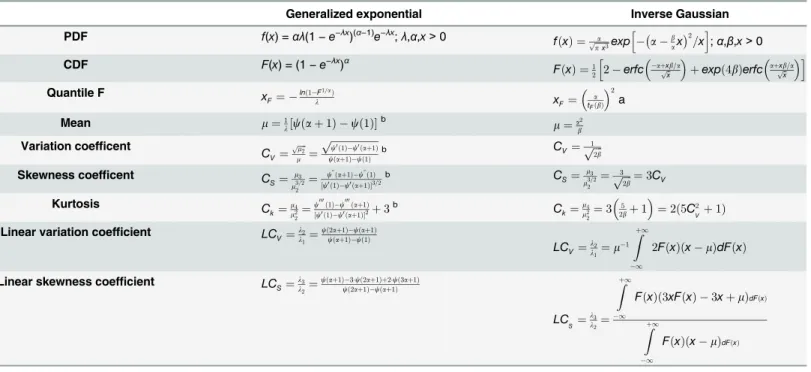
The basic statistical characteristics of both IG and GE distributions are presented inTable 3. The polygamma functions are defined as the logarithmic derivative of the gamma function [37]:

cðnÞðzÞ ¼ d n

dzncðzÞ ¼

dnþ1

dznþ1ln½Gðzފ for n¼1;2;3;. . . ð4Þ

For real positive argumentsz, digamma functionψ(z) is a concave increasing function ofz

which satisfies the following relation [37], [38]:

cðzÞ ¼lnðzÞ ₂1

z

1

12_z2þ

1

120_z4

1

252_z6þ

1

240_z8

1

132_z10þO

1

z12

ð5Þ

DifferentiatingEq 5appropriate number of times, one gets the evaluations of polygamma func-tions that can be used for numerical calculafunc-tions instead of analytical formulas.

Only the first two linear moments of GE distribution have been derived so far [20]. The for-mula for its third linear moment (λ₃) and thus for the linear skewness coefficient (LCS) has

been derived by the authors (seeAppendix) and presented inTable 3. Since the linear moments of IG distribution have no analytical form, their integral formulas are applied for computa-tional calculations and the trapezoidal rule is used for approximation of the definite integral [39]. The details concerning the derivation of the formula for the quantile corresponding to probabilities of non-exceedanceF(xF) for IG distribution are shown in [27].

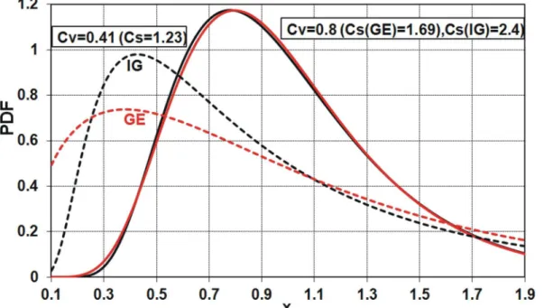
As shown inFig 4, for the variation coefficientCVequal to 0.41, the skewness coefficientsCS

of both GE and IG distributions are the same and amount to 1.23. As the two basic characteris-tics for the two-parameter distributions are equal, the shapes of distribution density functions are almost identical; see solid lines inFig 6. However, the PDFs are not identical, since the val-ues of kurtosisCK=μ4/μ2vary and equal to 5.67 and 3.68 for GE and IG distributions,

respec-tively. As you move away fromCV= 0.41, the differences in the values ofCSof both

distributions increase (Fig 4); therefore, the shapes of their density functions differ from each

Fig 6. Probability density functions of GE and IG distributions forμ= 1.0 and selected values ofCVand thusCS.

other. This is exemplified byCV= 0.8 and corresponds to the valuesCS= 1.69 andCS= 2.4 for

GE and IG distributions, respectively; see solid lines inFig 6.

Discrimination Procedures

The main disadvantage of using the wrong form of distribution for a flood series is that it over-or under-designs the hydraulic structures. Even if the sample size is not sufficiently large fover-or making a proper choice among alternative distribution functions, a selection method is still needed and moreover all available information should be utilized for it. To find the best fitting model to empirical data from the set of competing models, a discrimination procedure is required. It must define a test statistics as well as a decision rule indicating the action to be taken for the sample under consideration. One can also prioritize all competing models accord-ing to the values of the selection criterion. However, the use of a discrimination procedure without the knowledge of its performance for the considered set of PDFs may be“a foolhardy gamble”[40] and may lead to erroneous conclusions [21]. To increase the efficiency of the model selection techniques in FFA, the use of several discrimination procedures along with the knowledge of their efficiency for a particular case is advisable.

K

procedure

TheKprocedure [41], [42] of model selection is based on the likelihood functionsLi¼ N

j¼1fiðxjÞ fori= 1,. . ._{,kandkis the number of considered distributions expressed by their density functions}

fi. In fact, theKprocedure is equivalent to the Akaike information criterion (AIC) [43] for

distri-butions with the same number of parameters. The procedure points out the model with the high-est value of the logarithm of the likelihood function as the true or the closhigh-est to the true model among all competing models, i.e.:

max

i¼1;...;k max^_y lnLið

^ y_Þ

g

( #

ð6Þ 2

4

where^yis a set of distribution parameters evaluated by any estimation method. In this study, three methods of the assessment of parameters and, thus, offlood quantiles are applied, i.e. the method of moments (MOM) (e.g. [44]), the method of linear moments (LMM) (e.g. [19]), and the maximum likelihood method (MLM) (e.g. [45]). These methods were applied for the IG and GE distributions in [27] and [46], respectively. The accuracy of the estimates of large quantiles obtained from these three methods for the two- and three-parameter log-normal and GEV distri-butions have been analyzed in [47] both in the case of true and false hypothetical models, while the asymptotic bias of a quantile caused by the wrong distributional assumption has been analyti-cally derived for a wide set of two-parameter distributions in [48], [49] and [17].

QK

procedure

TheQKdiscrimination procedure bases on the statistics that is invariant under scale transfor-mation of the data [30]:

Si¼ Z 1

0

fiðlx1;. . .;lxNÞl N 1

dl _ð7Þ

whereNis the sample size andfiis the probability density function with scale parameter equal

considered distributions is estimated by the MLM method and substituted intoEq 7. As the selec-tion rule, Quesenberry and Kent [50] proposed to choose the model which corresponds to the highest value of theSistatistics among competing PDFs. They showed that theQKdiscrimination

procedure minimizes the sum of the probabilities of selecting the incorrect families of distribution. In practice the logarithm of the selection statisticsSiinstead of the statistics itself is usually applied:

max

i¼1;...;k½lnSiŠ ð8Þ

The analytical formula for the logarithms of theSistatistics of the inverse Gaussian

distribu-tion has been derived and published with small editorial error in [21]. Therefore, its corrected form is given below:

lnSIG¼lnð2Þ þ

N

2ln b p

þ2_Nb 3

2NlnðxÞ þ

N

4ðlnðxÞ lnðx

1 ÞÞþ þln ( KN 2

2_Nbpffiffiffiffiffiffiffiffiffiffiffiffiffi_xx 1

h i

g

whereKνis the modified Bessel function of the second kind (e.g. [37]). Since we failed to get the analyticalQKformula for the generalized exponential distribution, the selection statistics lnSGEhas been calculated numerically from the definitionEq 7using the trapezoidal rule for

approximation of the definite integral (e.g. [39]).

KS

procedure

TheKSprocedure employs the Kolmogorov-Smirnov statisticsDmax

i proposed by Kolmogorov [51]. The statistics is oriented to measure the goodness offit between the hypothetical and empirical distributions and, in terms of probability of exceedance, it has the form (e.g. [52]):

Dmax

i ¼_jmax

¼1_;..._;Njpiðxj:NÞ

^

p_j:_Nj ð10Þ

wherepi(xj:N) expresses the theoretical probability of thej-th element of the non-ascending

ordered random samplex1:N. . .xN:Nfrom thei-th distribution (in the set ofkalternative

distributions) and^_p

j:_Nis its empirical probability given here by the Weibull formula:

^

pj:_N ¼j=ðNþ1Þ ð11Þ

The model selected is the one which corresponds to the lowest value ofDmax

i function among all considered models, i.e.:

min i¼1;...;k½D

max

i Š ð12Þ

StatisticsDmaxis typically used as the test statistics in the Kolmogorov-Smirnov test of good-ness of fit a distribution to the data. An attractive feature ofDmaxis that its distribution does not depend on the underlying CDF being tested [53].

R

procedure

Since no simple statistical model can reproduce the dataset in its entire range of variability, it seems to be a right idea that the shape of the distribution tail should be a leading statistics when choosing a hypothetical distribution. Some guidelines and procedures for selecting the class of distributions that provides the best fit to the sample extremes are presented, for example, in [54–

TheRprocedure follows the thought of fitting the model to the data in the range of the distri-bution tail. The parametric methods of the estimation of a model density function are asymptoti-cally unbiased, which means that the assessment of any model parameter tends to its exact value for the sample withdrawn from the population of known distribution function. Then, in particular, the estimate of any quantile converges to its true value. Basing on this rule, the differences between the estimates obtained from various methods have been used to assess model fitting to the sample. The procedure of model discrimination has been explicitly proposed in [22] and based on the dif-ference between 1% quantile assessmentð^_x1

%Þprovided by the method of moments and the maxi-mum likelihood method. The 1% quantile assessment is the most commonly used design value and corresponds to a probability of exceedancep= 0.01 (i.e.F= 0.99), expressed as a percentage. According to the relation between the probability and return period (Eqs2and3), the^_x1

% deter-mines the probable maximumflow which appears, on average, once in 100 years.

Here, two discrimination statistics,R1

i andR

2

i, are proposed, fori= 1,. . .,kandkbeing the number of competing PDFs:

R1

i ¼ jx^ MLM

1_%ðiÞ x^

MOM

1_%ðiÞj ð13Þ

R2

i ¼ j^x MLM

1_%ðiÞ ^x

LMM

1_%ðiÞj ð14Þ

where_x^MOM

1%ðiÞ; ^xLMM1%ðiÞ; ^xMLM1%ðiÞare the 1% quantiles estimated by the moment method, the linear moments method and the maximum likelihood method, respectively. For both discrimination statistics (Eqs13and14), the best model is the one with their lowest value:

min i¼1;...;k½R

1

iŠ ð15Þ

min i¼1;...;k½R

2

iŠ ð16Þ

Note that for normal distribution the MOM and MLM methods are equivalent. Therefore, if the normal distribution is among the alternative distributions, it would be chosen by theR pro-cedure. What's more, all three estimation methods also give the same estimate of the mean for gamma and the two-parameter inverse Gaussian distributions. This gives for these distributions the similarity of the estimates of quantiles for these three methods in the range of the main prob-ability mass and, to a certain extent, for higher quantiles as well. Therefore, to use theR proce-dure properly, the knowledge of its performance for the considered set of PDFs is required.

Evaluation of Efficiency of Discrimination Procedures

Each discrimination procedure is considered to be of universal use, i.e. can be applied for model selection among any set of alternative PDFs, regardless of the sample size. However, the real drawback appears when for a small or medium sample size the discrimination procedures tend to favour some alternative distributions.

generated from the GE and IG distributions, respectively, for sample sizesN= 20, 50 and 100. To unify the distributions with respect to parameters, the original parameters were replaced by the meanμand the variation coefficientCV. Without a loss of generality, the mean equal to one

is assumed. The variation coefficient varies from 0.3 to 1.0; this covers the range ofCVvalues

for Polish data (seeFig 1). The results available in the literature [21], [22] indicate significant differences in the values of the PCS obtained by theKandQKdiscrimination procedures for different pairs of distributions and small sample sizes generated. A similar result was expected for the pair of distributions IG and GE. However, to our surprise, the values of PCS according to theKdiscrimination procedure (Fig 7) are almost identical to the values from theQK proce-dure (Fig 8). The differences between these two procedures are shown inFig 9.

The values of the probability of inconsistent selection(PIS) inFig 9mean that for a single sample generated from the assumed PDF, one of the procedures,KorQK, points out the right PDF (correct selection), while, at the same time, the latter procedure points out the wrong PDF (incorrect selection). In other words, the values of PIS are the percentages of inconsistency of the two procedures.

We have detected the identity of theKandQKprocedures for the pairs of the inverse Gauss-ian with log-normal or gamma distributions. This issue will be further investigated. However, it seems that theKandQKprocedures of discrimination are equivalent when IG is one of the alternative distributions, which is a unique feature of this distribution.

Finally, the results obtained from theKSand both variants ofRdiscrimination procedures, i.e.R1andR2, are presented in Figs10–12, respectively.

PCS for the pair of GE and IG distributions

It is quite clear from the above figures that the PCS increases with increasing sample size, i.e. the probability of correct selection is the smallest for 20-element samples and the highest for

Fig 7. Probability of correct selection [%] for competing GE and IG distributions by theKdiscrimination procedures.

100-element samples. The exception is theR2procedure applied for the true GE distribution with IG as an alternative within the range of variation coefficientCVfrom 0.3 to 0.45 (Fig 12).

It is also clear that asCVmoves away from the value around 0.4, the PCS increases. For all

Fig 9. Probability of inconsistent selection [%] for competing GE and IG distributions by theKorQKdiscrimination procedures. Fig 8. Probability of correct selection [%] for competing GE and IG distributions by theQKdiscrimination procedures.

considered discrimination procedures, if the variation coefficient is about 0.4, a sharp decline of the PCS value is visible. Only for theKSprocedure the decrease of PCS value is more evident when IG is the true sample distribution (Fig 10), while for the other procedures this effect is stronger when GE is the true sample distribution (Figs7,8,11and12). For example, for theK

andQKprocedures, when the data are drawn from the IG distribution, the PCS is about 63% at the minimum point for all the considered sizes of the sample, while if the data are drawn from the GE distribution, the PCS decreases up to about 34% for the sample sizeN= 20, i.e. then 66% of samples generated from GE distribution will be wrongly recognized as originated from IG parent distribution. The lowest value of the PCS among the GE and IG models forCV*0.4

is related with the fact that for the variation coefficient equal to 0.41, the skewness coefficients

CSof both distributions are the same and amount to 1.23. Hence, for the range ofCVaround

0.4, the investigated distributions have a similar shape, as shown inFig 6.

Similar results as for the proceduresKandQKare obtained for the procedureR(Figs11

and12). However, note that for the variantR2(Fig 12), the minimum of the PCS obtained for the case of T = GE and F = IG decreases below 30%. In general, if GE is the true sample distri-bution andCVis lower than 0.5, it does not make sense to use any variant ofRdiscrimination

procedure, since the probability of the correct selection of the distribution is lower than 50%. Then the decision based on“head and tail”rule is more efficient and easier to use. The same applies to the proceduresKandQKandCVabout 0.4, depending on the sample sizeN.

Fig 10. Probability of correct selection [%] for competing GE and IG distributions by theKSdiscrimination procedure.

For all four discrimination procedures, the generalized exponential model is better recogniz-able than the inverse Gaussian, for moderate and largeCVvalues, i.e.CV>0.5, while for small CVvalues, i.e.CV<0.5, the GE model is favoured only byKSprocedure (Fig 10) and IG model

is favoured byK,QKandRprocedures (Figs7,8,11and12).

For the range ofCVfrom 0.6 to 0.8, which covers most data of Polish Rivers, the probability

of correct selection among GE and IG distributions is quite large. Except of some cases of 20-element series drawn both from the IG and GE distributions, the PCS is higher than 70%. However, it should be remembered that the above experiment relates to a special theoretical case when one of the two competing distributions is the true one. If there are more alternative models, the probability of the selection of the true distribution significantly decreases. Simi-larly, the PCS is smaller if a set of alternative distributions consists of the PDFs which are simi-lar in type to the true distribution. Note, the exponential distribution is a special case of the gamma, Weibull and generalized exponential models, if the shape parameter is equal to one, being a special case of Pareto, if the shape parameter is equal to zero. Then the PCS among any pair of the distributions from the set above would be lower than the PCS among GE and IG distributions.

Fig 11. Probability of correct selection [%] for competing GE and IG distributions by theR1_{discrimination procedures.}

Asymptotic Model Error in Respect to the Upper Quantile

In flood frequency analysis, the assumed (hypothetical) model is treated as the correct (true) model and any assessment of the accuracy of the estimation of its parameters and quantiles is usually made assuming that the considered random sample is derived from that probability distribution. In this way, the error of the choice of false distribution, i.e. the model error, is omitted, although this error can have a significant impact on the accuracy of the quantiles esti-mation. For a given estimation method, the total bias of quantile estimate consists of a sam-pling bias which asymptotically converges to zero and a model bias caused by wrong

distributional selection. Those biases can be of opposite signs. The theoretical background for the asymptotic bias caused by false distributional assumption for various estimation methods has been presented in [48] followed by derivations for various pairs of (True, False) distribu-tions in [49], [17].

Here, the set of competing PDFs involves the generalized exponential and inverse Gaussian distributions and the interest is in the derivation of the asymptotic model bias of the 1% quan-tile estimate; when the GE is the true (T) population model, then the IG is falsely (F) adopted for the hypothetical PDF, and vice versa. Three estimation methods presented in section 3.1 are used as approximation method of T distribution by F distribution. The relative model bias

Fig 12. Probability of correct selection [%] for competing GE and IG distributions by theR2_{discrimination procedures.}

is defined for each approximation method as:

RBð^_x

1%Þ ¼ ^

x1_%ðF=TÞ ^x1_%ðTÞ

^

x1_%T

ð17Þ

To present a unified treatment for both distributions and three estimation methods, the mean of the T distribution equal to 1.0 and the variation coefficientCVvarying from 0.3 to 1.0

are considered in the experiment. The relative asymptotic bias of_x^

1%is determined analytically by the methods of MOM and LMM, while to use MLM, the samples of sizeN= 9000 have been generated from the GE and IG distributions, in turn. The results are presented in Figs13and14.

One can see that the incorrect choice of distribution for describing the chosen data series may lead to large errors of the 1% quantile estimate, especially if the maximum likelihood method is applied. For example, if the large sample from the GE distribution of the variation coefficientCV= 0.8 is falsely modelled by the IG distribution, then the relative asymptotic bias

of^_x1

%equals 7% and 16.2% for the MOM and LMM estimation methods, respectively, while it is nearly 66% for the MLM (Fig 13). In the opposite case, i.e. when the sample is derived from the IG distribution and the GE model is mistakenly assumed, the rank of estimation methods is similar, except that the bias sign is negative. ForCV= 0.8 and MLM estimation method, the RBð_x^_{1%Þis equal to -18.8%, while for LMM and MOM methods, theRBðx}^_{1%Þis equal to -12.2%} and -6.59%, respectively (Fig 14). The differences in the value ofRBð^_x1

%Þobtained from the MLM and two other estimation methods are significant, especially in the case of T = GE,

Fig 13. Relative asymptotic bias [%] ofx^

1%from T = GE distribution, assuming F = IG model.

F = IG (Fig 13), being lower in the case of T = IG, F = GE (Fig 14). Thisfinding essentially diminishes the practical usefulness of MLM in hydrological extremes analysis, because its effi-ciency may not compensate for the (frequently) large bias produced by the model misspecifica-tion, which is highly probable in hydrological reality.

Case Study

In order to analyze the GE and IG distributions fitting to the Polish data, four gauging stations have been selected as examples. These are Rudze, Stróża, Koszyce Wielkie and Wadowice sec-tions on the Wieprzówka, Raba, Biała and Skawa Rivers, respectively. Their basic characteris-tics are presented inTable 2under the numbers 15, 16, 26 and 14, in turn. All four stations are located in the mountain area in the south part of Poland (Fig 3) and are characterized by a high dynamics of flows. For each gauge, the 90-year series of annual maximum flows from the period 1921–2010 has been investigated. Both two-parameter models, namely GE and IG, have been used to reproduce the data series. The 1% quantile has been estimated by three estimation methods, MOM, LMM and MLM. To find the best fitted distribution among the two compet-ing PDFs, four discrimination procedures have been applied, namelyK,QK,KSandR. Since the alternative distributions contain the same number of parameters, any procedure of model selection can be used for the assessment of the best fitting model. However, for a group of PDFs containing both two- and three-parameter functions, a discrimination procedure which takes into account the number of model parameters should be used, such as, for example, the

Fig 14. Relative asymptotic bias [%] ofx^

1%from T = IG distribution, assuming F = GE model.

Akaike information criterion (e.g. [43], [57]). Otherwise, the three-parameter distribution would always be better than their counterpart two-parameter models.

Accuracy of the fit of models

The values of 1% quantile estimates for selected gauging stations are presented inTable 4. For each section, the values of_x^₁

%differ significantly between the distributions, when the MLM method is used for their estimation, while the differences are the smallest when the MOM method is applied. Generally, while estimating the upper quantiles, the MLM is the most sensitive in respect to model choice and the MOM is the most stable estimation method. Tofind which of the distributions is the bestfitting for each annual maximumflow series and, in particular, tofind which of the estimates of 1% quantile is the most reliable, the four proce-dures of discrimination are applied and their results are shown inTable 5. The bold font on a gray background means that for particular gauging stations the model is the bestfitted among two alternative PDFs.

For the Rudze gauging station, all four procedures of discrimination point out the general-ized exponential distributions as better fitted than the inverse Gaussian. The same is true for the Stróża station, with the exception of theKSdiscrimination procedure and the MLM estima-tion method when the IG distribuestima-tion fits to the data series better. For the Koszyce and

Table 5. Distribution choice by the four discrimination procedures for annual maximum records of selected gauging stations.

Discrimination procedure Estimation method Rudze Rudze Stróża Stróża Koszyce Koszyce Wadowice Wadowice

GE IG GE IG GE IG GE IG

Kprocedure MOM -451.54 -482.78 -565.82 -568.16 -587.89 -589.08 -582.13 -580.29

LMM -450.00 -466.66 -565.95 -566.18 -588.30 -586.47 -582.17 -579.51 MLM -449.86 -457.33 -565.60 -565.73 -587.80 -586.27 -581.53 -579.49

QKprocedure MLM -451.39 -458.78 -567.27 -567.36 -589.44 -587.89 -583.23 -581.17

KSprocedure MOM 0.1052 0.1500 0.0670 0.0733 0.1097 0.1219 0.0656 0.0850

LMM 0.0933 0.1282 0.0640 0.0712 0.0958 0.0776 0.0647 0.0651 MLM 0.0918 0.1656 0.0762 0.0704 0.1181 0.0755 0.0913 0.0652

Rprocedure R1 20.298 117.29 30.989 132.82 26.929 183.13 61.871 91.181

R2 6.8190 82.382 38.889 61.935 60.540 54.553 63.859 16.917

doi:10.1371/journal.pone.0143965.t005

Table 4. The 1% quantile estimates for selected gauging stations in Poland, assuming GE and IG dis-tributions, respectively.

Gauging station Estimation method x^

1%(GE) x^1%(IG)

Rudze MOM 200.08 212.81

LMM 213.56 247.71

MLM 220.38 330.09

Stróża MOM 787.69 838.02

LMM 795.59 908.90

MLM 756.70 970.84

Koszyce MOM 1000.7 1065.0

LMM 1034.3 1193.5

MLM 973.80 1248.1

Wadowice MOM 956.85 1017.1

LMM 958.83 1091.4

MLM 894.97 1108.3

Wadowice sections, the choice of the best fitting model varies greatly, depending on the dis-crimination procedure and the estimation methods. In the case of the Koszyce station, in most variants of procedure and method (6 out of 9 cases), the IG distribution is pointed out as the better fitted than the GE. The superiority of the IG distribution over the GE is indicated only by theKandKSprocedures along with the MOM method and by the variantR1of theR proce-dure. Similarly, the data series from the Wadowice gauging station should be modelled using IG distribution rather than GE, according to theK,QK,KSprocedures with the MLM method and the variantR2of theRprocedure. In the other three cases, the GE distribution over the IG distribution is favoured.

Despite the similar hydrological regime and the same observation period, for each gauging station, the best fitted model depends on the discrimination procedure and the estimation method. However, as shown above, the superiority of GE distribution over the previously dom-inant IG distribution, detected in many cases, proves that GE occupies one of the leading posi-tions among distribuposi-tions commonly used in flood frequency modelling of Polish data.

Aggregation of models

The results of PCS studies and discrimination procedures confirm our belief as to the uncer-tainty of the identification of the true distribution type among alternative distributions. Besides, the general considerations lead to the conclusion that the true distribution type is beyond the cognitive capabilities. Even if the true distribution exists, it would probably have countless parameters, unidentifiable from the available observation series. In summary, we are inclined to believe that, for a set of alternative models, the quantile estimate obtained from each model contains a piece of information about the true quantile value. This piece of result should be provided with a proper weight, depending on the quality of the fit of a particular model to the data series. Such a multi-model approach (called“aggregation”) in the estimation of the extreme value distribution quantiles has been presented by Bogdanowicz [23]. The aggregated quantileðxp%Þis defined as a sum of quantiles estimated by MLM method for each of alternative distributions multiplied by their weightswi. The weights are defined using the

likelihood function:

wi ¼

Li

Xk

m¼1

Lm

fori¼1_;. . ._{;k ð18Þ}

Eq 18is valid for the case when all distribution candidates have the same number of parame-ters; otherwise, the Akaike information criterion is applied for the definition of the distribution weights. The weights can be interpreted as the conditional probability of the adequacy ofi-th model, so the aggregated quantile is a conditional expected value.

The aggregation data for four investigated gauging stations are presented inTable 6. The estimates of upper quantiles obtained from the aggregation method seem to be more reliable and stable than from the classical approach, since the aggregation allows to partly over-come the problem of the arbitrary choice of the best fitted model. Moreover, the aggregation of models mitigates the problem of fluctuations of the upper quantile estimates, used as the hydrological design value along the river.

Summary and Conclusions

the annual maximum flow series for Polish Rivers reveals that the inverse Gaussian and gener-alized exponential distributions seem to be a desirable complement.

Applying a discrimination procedure without the knowledge of its performance for the con-sidered PDFs may lead to erroneous conclusion and finally to erroneous quantile estimates. The experiment on the probability of correct selection (PCS) reveals that the values of PCS are fairly high forK,QK,KSandRprocedures of discrimination. However, they sharply decrease in the vicinity of the variation coefficient 0.4. Applying theK,QKandRprocedures, the PCS is even lower than 50% if the GE is the true sample distribution, being higher than 60% if the IG is the true sample distribution. If the probability of selection of the right PDF is mostly much lower than 50%, which is observed here for the range ofCVbetween 0.3 and 0.5, it does not

make sense to employ the sophisticated procedures of discrimination, since a simple“head and tail”rule is more efficient and easier to use. However, for the range ofCVfrom 0.6 to 0.8, which

covers most data of Polish Rivers, the probability of correct selection among GE and IG distri-butions is quite large for all four discrimination procedures, being higher than 70% for moder-ate and large sample sizes.

The analysis of fitting the generalized exponential and inverse Gaussian distributions to the 90-year series of annual maximum flows for four selected gauging stations in Poland, reveals that the assessment of 1% quantile differs considerably for various models and estimation methods. The choice of the best fitting model (distribution type and its parameter values) is not unique. It depends on the discrimination procedure used (criterion for the selection of the distribution) and the method of estimation. It is characteristic for hydrological size of samples. The results from four procedures of discrimination applied to modelling of annual peak flow series for four Polish gauging stations show in many cases the superiority of GE distribution over IG distribution, which has been dominant in FFA in Poland so far. This shows that GE occupies one of the leading positions among distributions commonly used in flood frequency modelling of Polish data and can be included into the group of the alternative distributions. The solution to the problem of the choice of the best fitting model can be the aggregation of quantiles obtained from all candidate distributions.

Despite the use of multiple distributions for flood frequency analysis, there is still a room for new models. However, one should remember that the choice of the distribution is just one aspect of the modelling of flood frequency, besides the choice of the estimation method and discrimination procedures. As shown in the paper, the selection of each of the above elements does have a significant impact on the estimate of desirable quantile. Moreover, note that the proliferation of statistical techniques causes the heterogeneity of results and finally leads to an increase the uncertainty of flood quantile estimates, instead of leading to clear solution. This stands in contrast with the expectation of engineers and hydrologists as they want to have a unique value, not accepting the uncertainty.

Table 6. The aggregation of 1% quantile of annual maximum flow series for selected gauging stations in Poland.

Gauging station weight weight x^

1%(GE) x^1%(IG) x1%

GE IG

Rudze 0.9994 0.0006 220.38 330.09 220.44

Stróża 0.5325 0.4675 756.70 970.84 856.81

Koszyce 0.1784 0.8216 973.80 1248.1 1199.2

Wadowice 0.1150 0.8850 894.97 1108.3 1083.8

Appendix

Derivation of the third linear moment

λ

for GE distribution

The cumulative distribution function of the three-parameter generalized exponential distribu-tion has the form:

FðxÞ ¼ ð1 _e lðx εÞ_Þa

ðA:1Þ

whereε,λ,α>0 are the location, scale and shape parameters, respectively. Hence we get the following quantile:

x¼ε lnð1 F

1₌a_Þ

l ðA:2Þ

The third linear moment can be defined using the formula [19]:

l3¼6b2 6b1þb0 ðA:3Þ

whereβ_r, forr= 0,1,2,. . ._{, are the probability weighted moments of a random variable:}

b_r¼ Z þ1

1 xFr

ðxÞdFðxÞ ðA:4Þ

Substituting EqsA.1andA.2toEq A.4forr= 0,1,2, we get the probability weighted moments of forms:

b0¼m¼εþ

c_ða_þ1_Þ c_ð1_Þ

l ðA:5Þ

b1 ¼

1

2 εþ

cð2_aþ1_{Þ cð}1_Þ l

ðA:6Þ

b2 ¼

1

3 εþ

c_ð3a_þ1_Þ c_ð1_Þ l

ðA:7Þ

whereψis the digamma function [37], [38].

Finally, after substituting EqsA.5–A.7intoEq A.3and after some simplifications, the for-mula of the third linear moment for GE distribution has a form:

l3 ¼

cðaþ1_Þ 3_cð2_aþ1_{Þ þ}2_cð3_aþ1_Þ

l ðA:8Þ

Supporting Information

S1 Table. Abbreviations and symbols commonly used in the paper. (DOC)

Author Contributions

References

1. Gumbel EJ. The return period of flood flows. Ann Appl Stat. 1941; 12(2):163–190.

2. Moran PAP. The statistical treatment of flood flows. Eos (Washington DC). 1957; 38(4):519–523.

3. Benson MA. Uniform flood frequency estimating methods for federal agencies. Water Resour Res. 1968; 4(5):891–908.

4. Jenkinson AF. Statistics of extremes. Estimation of maximum floods. WMO No 233, TP126, Tech. Note No. 98. Geneva, Switzerland: Secretariat of the World Meteorological Organization; 1969. 183–228 pp.

5. Beard LR. Flood flow frequency techniques. The University of Texas at Austin: Center for Research in Water Resources; 1974.

6. NERC. Flood Studies Report Volume 1: Hydrological Studies. London: Natural Environment Research Council; 1975.

7. Boughton WC. A frequency distribution for annual floods. Water Resour Res. 1980; 16(2):347–354.

8. Cunnane C. Statistical distributions for flood frequency analysis. Operational Hydrology Report No.33. Geneva: World Meteorological Organization; 1989.

9. [Guidelines for determination of the annual maximum flows with the assumed probability of occurrence for the designing of engineering and hydrotechnical devices in hydraulic engineering]. Warsaw: Cen-tralny Urząd Gospodarki Wodnej (CUGW); 1969. Polish.

10. Adler RJ, Feldman RE, Taqqu MS. A practical guide to heavy tails: Statistical techniques and applica-tions. Birkhauser; 1998.

11. FEH. Flood Estimation Handbook. Institute of Hydrology. Wallingford, Oxfordshire OX10 8BB, United Kingdom: 1999.

12. Rao AR, Hamed KH. Flood frequency analysis. Boca Raton, Florida, USA: CRC Press; 2000. 13. Katz RW, Parlange MB, Naveau P. Statistics of extremes in hydrology. Adv Water Resour. 2002;

25:1287–1304.

14. Griffis VW, Stedinger JR. Evolution of flood frequency analysis with Bulletin 17. J Hydrol Eng. 2007; 12 (3):283–297.

15. Review of applied European flood frequency analysis methods. Floodfreq Cost Action ES0901. Euro-pean procedures for flood frequency estimation. Centre for Ecology and Hydrology on behalf of COST. ISBN: 978-1-906698-32-4. 2012.

16. Rowiński PM, Strupczewski WG, Singh VP. A note on the applicability of log-Gumbel and log-logistic probability distributions in hydrological analyses: I. Known pdf. Hydrol Sci J. 2002; 47(1):107–122.

17. Węglarczyk S, Strupczewski WG, Singh VP. A note on the applicability of log-Gumbel and log-logistic probability distributions in hydrological analyses: II. Assumed pdf. Hydrol Sci J. 2002; 47(1):123–137.

18. Strupczewski WG, Kochanek K, Markiewicz I, Bogdanowicz E, Węglarczyk S, Singh VP. On the tails of distributions of annual peak flow. Hydrol Res. 2011; 42(2–3):171–192. doi:10.2166/nh.2011.062

19. Hosking JRM, Wallis JR. Regional frequency analysis. An approach based on L-moment. Cambridge CH2 1RP, United Kingdom: Cambridge University Press; 1997.

20. Gupta RD, Kundu D. Generalized exponential distribution: existing results and some recent develop-ments. J Stat Plan Inference. 2007; 137(11):3537–3547. doi:10.1016/j.jspi.2007.03.030

21. Strupczewski WG, Mitosek HT, Kochanek K, Singh VP, Węglarczyk S. Probability of correct selection from lognormal and convective diffusion models based on the likelihood ratio. Stoch Environ Res Risk Assess. 2004; 18:1–11. doi:10.1007/s00477-004-0210-8

22. Mitosek HT, Strupczewski WG, Singh VP. Three procedures for selection of annual flood peak distribu-tion. J Hydrol. 2006; 323:57–73. doi:10.1016/j.jhydrol.2005.08.016

23. Bogdanowicz E. [Multimodel approach to estimation of extreme value distribution quantiles]. Mono-graphs of Committee Environmental Engineering Polish Academy of Sciences: Hydrology in Engineer-ing and Water Management. 2010; 68(1): 57–70. Polish.

24. Cox DR, Miller HD. The Theory of Stochastic Processes. London: Chapman and Hall; 1965. 25. Hayami S. On the propagation of flood waves. Bulletins—Disaster Prevention Research Institute at

Kyoto University. 1951; 1:1–16.

26. Dooge JCI. Linear theory of hydrologic systems. Technical Bulletin No. 1468. Washington D.C.: Agri-cultural Research Service, U.S. Department of Agriculture; 1973.

27. Strupczewski WG, Singh VP, Węglarczyk S. Impulse response of linear diffusion analogy model as a flood frequency probability density function. Hydrol Sci J. 2001; 46(5):761–780.

29. Strupczewski W. G., Singh V. P., Węglarczyk S. and Mitosek H. T. Physics of flood frequency analysis. II. Convective diffusion model versus lognormal model. Acta Geophys Pol. 2003; 51(1):85–106.

30. Hájek J,Šidák Z. Theory of Rank Tests. New York: Academic Press; 1967.

31. Gupta RD, Kundu D. Generalized exponential distributions. Aust N Z J Stat. 1999; 41(2):173–188. doi:

10.1111/1467-842X.00072

32. Gupta RD, Kundu D. Discriminating between the Weibull and the GE distributions. Comput Stat Data Anal. 2003; 43:179–196.

33. Gupta RD, Kundu D. Closeness of gamma and generalized exponential distribution. Commun Stat The-ory Methods. 2003; 32(4):705–721.

34. Gupta RD, Kundu D. Discriminating between gamma and generalized exponential distributions. J Stat Comput Simul. 2004; 74(2):107–121.

35. Kundu D, Gupta RD, Manglick A. Discriminating between the log-normal and generalized exponential distribution. J Stat Plan Inference. 2005; 127:213–227.

36. Brzezinski J. [Application of generalized exponential distribution in seasonal maximum annual flow analysis]. Monographs of Committee Environmental Engineering Polish Academy of Sciences: Hydrol-ogy in Engineering and Water Management. 2010; 68(1):71–82. Polish.

37. Abramowitz M, Stegun IA. Handbook of mathematical functions. Tenth Printing. New York: Dover Pub-lications; 1972. 259–260 and 374–376 pp.

38. Bernardo JM. Algorithm AS 103 psi (digamma function) computation. Appl Stat. 1976; 25:315–317.

39. Atkinson EK. An introduction to numerical analysis ( 2nd ed.). New York: John Wiley and Sons; 1989. 40. Dyer AR. Discrimination procedures for separate families of hypotheses. J Am Stat Assoc. 1973; 68

(344):970–974.

41. Kappenman RF. On method for selecting a distributional model. Commun Stat Theory Methods. 1982; 11:663–672.

42. Kappenman RF. A simple method for choosing between the lognormal and Weibull models. Stat Pro-bab Lett. 1989; 7:123–126.

43. Akaike H. A new look at the statistical model identification. IEEE Trans Automat Contr. 1974; 19 (6):716–723. doi:10.1109/TAC.1974.1100705

44. Kendall MG, Stuart A. The advanced theory of statistics. Vol. 1. Distribution theory. London: Charles Griffin and Company Limited; 1969.

45. Kendall MG, Stuart A. The advanced theory of statistics. Vol. 2. Inference and relationship. London: Charles Griffin and Company Limited; 1973.

46. Gupta RD, Kundu D. Generalized exponential distribution: Different method of estimations. J Stat Com-put Simul. 2001; 69(4):315–337. doi:10.1080/00949650108812098

47. Markiewicz I, Strupczewski WG, Kochanek K. On accuracy of upper quantiles estimation. Hydrol Earth Syst Sci. 2010; 14:2167–2175. doi:10.5194/hess-14-2167-2010

48. Strupczewski WG, Singh VP, Węglarczyk S. Asymptotic bias of estimation methods caused by the assumption of false probability distribution, J Hydrol. 2002; 258:122–148,

49. Strupczewski WG, Węglarczyk S, Singh VP. Model error in flood frequency estimation, Acta Geophys Pol. 2002; 50(2):279–319.

50. Quesenberry CP, Kent J. Selecting among probability distributions used in reliability. Technometrics. 1982; 24(1):59–65.

51. Kolmogorov A. [On theempiricaldetermination of a distribution law]. Giornale d Insitute Italiano Attuari. 1933; 4:83–91. Italian.

52. Kaczmarek Z. Statistical methods in hydrology and meteorology. Published for the Geological Survey, U.S. Department of the Interior and the National Science Foundation, Washington, D.C., by the Foreign Scientific Publications Department of the National Centre for Scientific. Warsaw, Poland: Technical and Economic Information; 1977. 240 p.

53. Chakravarti IM, Laha RG, Roy J. Handbook of methods of applied statistics, Vol. I. New York: John Wiley and Sons; 1967. 392–394 pp.

54. Adlouni SEl, Bobée B, Ouarda TBMJ. On the tails of extreme event distributions in hydrology. J Hydrol. 2008; 355(1–4):16–33. doi:10.1016/j.jhydrol.2008.02.011

56. Dey AK, Kundu D. Discriminating Among the Log-Normal, Weibull, and Generalized Exponential Distri-butions. IEEE Trans Rel. 2009; 58(3):416–424.