Image Denoising with Modified Wavelet Feature Restoration
Sachin Ruikar1, Dharmpal Doye2
1
Research Scholar, Electronics and Telecommunication Department, SGGSIET Nanded, Maharashtra, India
2
Professor, Electronics and Telecommunication Department, SGGSIET Nanded, Maharashtra, India
Abstract
Image denoising is the principle problem of image restoration and many scholars have been devoted to this area and proposed lots of methods. In this paper we propose modified feature restoration algorithm based on threshold and neighbor technique which gives better result for all types of noise. Because of some limits of conventional methods in image denoising, several drawbacks are seen in the conventional methods such as introduction of blur and edges degradation. Those can be removed by using the new technique which is based on the wavelet transforms. The shrinkage algorithms like Universal shrink, visue shrink, bays shrink; have strengths in Gaussian noise removal. Our proposed method gives noise removal for all types of noise, in wavelet domain. It gives a better peak signal to noise ratio as compared to traditional methods
Keywords: Image Noise, threshold, Wavelet.
1. Introduction
Image Denoising consists of an attempt to recover an image which has been degraded by a linear shift-invariant filtering operation with noise. It has applications in fields such as astronomy, remote sensing and biomedical imaging as well as in everyday life for the enhancement of noisy photos. The existing linear image restoration of algorithms assumes that the Point Spread Function (PSF) is known a priori and it attempts to reverse it in cooperation to reduce noise by utilizing the available information. Although many researchers have worked on this type of problem, it was difficult to work with the unknown noise in many real situations [1].
The image restoration process is restoring an unknown image using partial or no information about the imaging system. It is well known that the image restoration is quite a challenging problem in the field of image processing, especially for those images which are degraded by Gaussian noise. The traditional method for image restoration is to detect the parameters of the PSF firstly from the degraded image, and then to recover the
underlying image. However, the restoration of the Gaussian noise image is very difficult, especially in the case of PSF unknown.
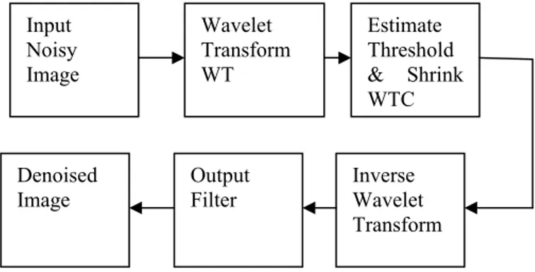
In [2] [3] Donoho proposes different thresholding technique, but this technique not keep details like edges, to overcome this we proposes new technique. In this paper, we have proposed the threshold and convolution technique. The input image is applied to different noises to get the noisy image. Different types of noise such as white Gaussian, Salt and Pepper, Speckle and Poisson’s added to the image .This image is transformed into the wavelet domain [4][5].The Wavelet features are modified by the proposed technique and process which would be reversed by applying Inverse Wavelet Transform to remove the noise from the image. Figure 1, elaborates the process of denoising Image denoising algorithm consists of a few steps, let us consider an input signal x(t) and noisy signal n(t), add both the signals to get y(t) , i.e.
)
(
)
(
)
(
t
x
t
n
t
y
(1) where the noise can be Gaussian, Poisson’s, speckle andSalt and pepper, then apply wavelet transform to get w(t).
)
(
)
(
t
w
t
y
Wavelet
Transform
(2) Modify the wavelet coefficient w(t) using different threshold algorithm and take inverse wavelet transform to get denoising image
x
ˆ
(
t
)
.ˆ
( )
Inverse Wavelet Transform( )
w t
x t
Fig. 1: Block diagram of denoising technique
2. Wavelet Transform
The wavelet expansion set is not unique. A wavelet system is a set of building blocks to construct or represent a signal or function. It is a two dimensional expansion set, usually a basis, for some class one or higher dimensional signals [7] [8] [9].
The wavelet can be represented by a weighted sum of shifted scaling function
(
2
t
)
as,
nn
t
n
h
t
)
(
)
2
(
2
)
n
Z
(
1
(4)For some set of coefficient h1 (n), this function gives the
prototype or mother wavelet
(
t
)
for a class of expansion function of the form)
2
(
2
)
(
/2,
t
t
k
j j k
j
(5) Where
2
jis the scaling oft
,
2
jk
is the translation int
, and2
j/2 maintains theL
2 norms of the wavelet at different scales. The construction of wavelet using the set of scaling function
k(
t
)
and
j,k(
t
)
that could span allof
L
2(
R
);
therefore functiong
(
t
)
L
2(
R
)
can be written as
k j k
k j
k
t
d
j
k
t
k
c
t
g
0 ,(
)
)
,
(
)
(
)
(
)
(
(6)First summation in the above equation gives a function that is low resolution of g (t), for each increasing index j in the second summation, a higher resolution function is added which gives increasing details. The function d(j,k) indicates the differences between the translation index k, and the scale parameter j. In wavelet analysis expand coefficient at a lower scale level to higher scale level, from equation (7), we scale and translate the time variable to give
n j n t tn
k
t
n
h
n
k
t
n
h
k
t
)
2
2
(
2
)
(
)
2
(
2
(
2
)
(
)
2
(
1
(7)After changing variables m=2k+n, the above equation becomes
m j tm
t
k
m
h
k
t
)
(
2
)
2
(
2
12
(
(8)At one scale lower resolution, wavelets are necessary for the detail not available at a scale of j. We have
k t j j j j k jk
t
k
d
k
t
k
c
t
f
)
2
(
2
)
(
)
2
(
2
)
(
)
(
2 / 2 /
(9)Where the
2
j/2 terms maintain the unity norm of the basic functions at various scales. If
j,k(
t
)
and)
(
,k
t
j
are orthonormal, the j level scaling coefficients are found by taking the inner product
f
t
t
f
t
t
k
dt
k
c
j(
)
(
),
j,k(
)
(
)
2
j/2
(
2
j)
(10)
By using equation (10) and interchanging the sum and integral, can be written as
m
j j
j
k
h
m
k
f
t
t
m
dt
c
(
)
(
2
)
(
)
2
( 1)/2
(
2
1)
(11) But the integral is an inner product with the scaling function at a scale
j
1
giving
m
j
j
k
h
m
k
c
m
c
(
)
(
2
)
1(
)
(12)The corresponding wavelet coefficient is
m
j
j
k
h
m
k
c
m
d
(
)
1(
2
)
1(
)
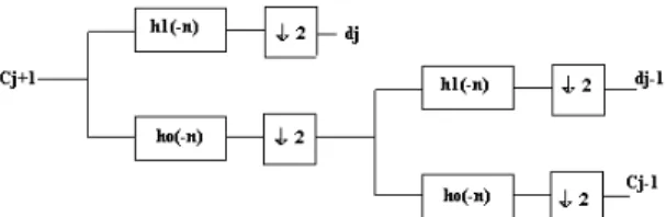
(13)Fig. (2) shows the structure of two stages down sampling filter banks in terms of coefficients.
Fig. 2: Two stages down sampling Filter bank
considering a signal in the j+1 scaling function space
f
(
t
)
v
j1. This function is written in terms of the scaling function as
k
j j
j
k
t
k
c
t
f
(
)
(
)
2
( 1)/2(
2
1)
1
(14)In terms of the next scales require wavelet as
k
j j j k
j j j
k
t
k
d
k
t
k
c
t
f
)
2
(
2
)
(
)
2
(
2
)
(
)
(
2 / 2 /
(15)
m j m
j
j
k
c
m
h
k
m
d
m
h
k
m
c
1(
)
(
)
(
2
)
(
)
1(
2
)
(16) Fig. (3) shows the structure of two stages up sampling filter banks in terms of coefficients i.e. synthesis from coarse scale to fine scale one [5] [6] [7].
Fig. 3: Two stages up sampling filter
The filter structure analysis can be done by applying one step of the one dimensional transform to all rows, then repeating the same for all columns then proceeding with the coefficients that result from a convolution within both directions, this is one level wavelet decomposition that proceeds similar for two levels for LL components to get a two-level decomposition structure shown in Fig. (4).
Fig. 4: Two-dimensional wavelet transforms
Calculating wavelet coefficients at every possible scale is a fair amount of work, and it generates an awful lot of data. We choose only a subset of scales and positions at which to make our calculation. It turns out, rather remarkably, that if we chose only a subset of scales and positions based on powers of two so-called dyadic scales and positions then our analysis will be much more efficient and just as accurate. We obtain such an analysis from the discrete wavelet transform [10] [11] [12].
3. Proposed Thresholding
generally suppress the details and edges of the original signal and cause blurring and ringing artifacts.
3.1 Proposed Threshold 1:
The image features are characterized by mean and standard deviation. The mean smoothen the image data reduces noise. Noise in an image logarithmically reduces. We propose nonlinear threshold operator for removing noise. This threshold is generated as
)
log(
2
m
M
newth
(17) Where, is the total number of pixel of an image, is the mean of the image. This function preserves the contrast, edges, background of the images. This threshold function is calculated at different scale levels. This proposed threshold performance calculated using peak signal to noise ratio (PSNR). A simple but often used quantitative measure of assessing image distortion due to degradation is the signal to noise ratio (SNR). The disadvantage with this measure of the SNR is that it is a function of the image variance. Even if the mean square error (MSE) between the two images is the same, SNR values can differ if the corresponding variance differs. Another quantitative measure often used in practice is peak SNR (PSNR), which is defined as the ratio of the square of the peak signal to the MSE, expressed in dB
MSE
peak
PSNR
2 10log
10
N n M mn
m
x
n
m
x
MN
MSE
1 1])
,
[
ˆ
]
,
[
(
1
Where, is the original image detail, and is the recovered image detail.
3.2 Circular kernel
Kernel applied to the wavelet approximation coefficient, to get de-noised image with all parameters is undisturbed. The kernel used here in this technique contains some components are zeros and ones as shown in Fig. (5).
A multi-resolution analysis wavelet structure has been used for this kernel to get result. This kernel helps to preserve the edges and boundary of the images so that better technique as compare to the other threshold methods. This kernel is used at the different decomposition level simply moving this window in an image. This step is called as convolution. The kernel has little degradation and enhancing components will not affect the original information of the image. It preserves the detail of the image. After convolution we have to
apply inverse wavelet to get denoisy image. This convolution method gives better peak signal to noise ratio (PSNR).
Fig. 5: Circular Kernel
3.3 Mean-Max threshold:
This method generates the threshold using mean and max method after wavelet decomposition at different level. Let xi denote the sequence of elements; threshold can be calculated using following technique.
)]
,...
(
[
....
)],
,...
(
[
)],
,...
(
[
1 1 2 1 i k i k k jx
x
MIN
x
x
MIN
x
x
MIN
MAX
x
MAXMIN
(18)
)]
,...
(
[
....
)],
,...
(
[
)],
,...
(
[
1 1 2 1 i k i k k jx
x
MAX
x
x
MAX
x
x
MAX
MIN
x
MINMAX
(19)This methodology gives MIN and MAX of the sub band at different level of the decomposed image. Then wavelet coefficients are threshold by different combination at different decomposition level. This threshold gives better PSNR for different noisy images.
3.4 Nearest neighbor:
value at that position [20]. The neighbor values 1,2,3,4 denote the components of the kernel will be marked as one. This mask is moving in the different sub band of the decomposed image. Then degraded coefficients are enhanced in this technique. These three kernels give better PSNR as compared to all technique at different noise level.
Fig. 6: Kernel at different noise level
3.5 Proposed Threshold 2:
For the image degradation depends on the standard deviation, mean, variance of image. Concentrating on the parameter we have proposed a new technique of threshold algorithm and to get the good results for the different noisy and blurred structures.
)
.
log(
energy
std
dev
mean
(20)
This threshold gives better PSNR performance parameter. For all types of noise image quality is drastically improved. This threshold is applied independently to each sub-band of an image’s wavelet coefficients using soft thresholding, including the lowest resolution LL sub-band. This yields a frequency adaptive threshold that is more aggressive in the signal. Use of this threshold optimizes performance by removing the most noise possible while still preserving the original signal.
3.6 Cluster average Technique
This technique applies to the features of the wavelet and is modified on the basis of the best suit by the technique of neighbor of cluster. The best basis determined from wavelet feature is as
ii
X
y
avg
1
3
/
1
)
(
(21)Replace the new value using
store
min(
avg
(
y
i))
Fig. 7: neighbor pixel
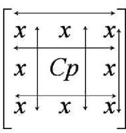
In Fig. (7) the center pixel CP will be replaced by taking
minima of all averages in all dimensions. This 3*3 neighbor varies in the full image and modified the wavelet coefficient at different level. The modified wavelet feature is obtained using the above method applied to the frequency domain. This technique gives a better PSNR of denoised image. This clustering is applied to independently to each sub-band at different level of decomposition. The wavelet coefficients using this neighboring at each level is modified and gives the denoised image by inverse wavelet transform.
4. Implementation and Result
Noise reduction plays a fundamental role in image processing, and wavelet analysis has been demonstrated to be a powerful method for performing image noise reduction. The procedure for noise reduction is applied on the wavelet coefficients achieved using the wavelet decomposition and representing the image at different scales. After noise reduction, the image is reconstructed using the inverse wavelet transform. A degraded noisy image can be approximately described using equation (1); this noisy image is obtained by using all noisy functions. Wavelet transform tool is applied to noisy image to get wavelet coefficient, the steps of algorithm are as follows i) Read an image.
ii) Apply different types of noise such as Gaussian, Poisson’s, speckle and Salt and pepper etc.
iii)Apply wavelet transform to noisy image at a required level, we would get four components namely, Approximation, Horizontal, Vertical, Diagonal coefficients.
v) In denoising each coefficient is threshold by comparing against a threshold; if the coefficient is smaller than the threshold it is set to zero, otherwise, it is kept
.
vi)Apply Inverse Wavelet transform to threshold coefficient, it gives a de-noised image.
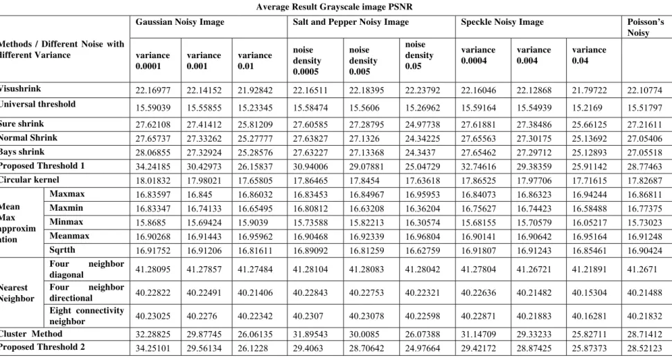
We have considered here ten images Result of all functions shown in Table (1) for all type of noise. Then we will recover the denoised image. We compared various denoising method on several test images widely used in image processing community. Here, we report the result only for the Lena image. The result shown in Fig. (8) shows graphical representation functions and their PSNR for Gaussian noisy image , Fig. (9) shows graphical representation functions and their PSNR shows the result for Salt and pepper noisy image, Fig. (10) shows the graphical representation functions and their PSNR shows the result for Speckle noise image. Fig. (11) shows graphical representation functions and there PSNR depicts the result of Poisson’s noise image.
5. Conclusion
The method describes a new way of denoising the image based on the wavelet transform. Because of some limits of conventional methods in image denoising, several drawbacks such as edge degradation are seen in the conventional methods. Those can be removed by using the new technique which is based on the wavelet transforms. We have analyzed the various techniques of image denoising by using the proposed methods. The proposed method 1 and proposed method 2 has good result at different noise level as compared to the existing methods. The circular kernel and Min Max method gives the better result visually but the PSNR is not good for this method as compared to all methods. This technique preserves the details of the image like edges as compared to the existing technique. The nearest neighbor method has better result as compared to the all existing method as well as all proposed technique. The cluster averaging technique has comparable excellent PSNR values. For Gaussian noise, all functions work better than the existing threshold. In Speckle noise, nearest neighbor methods give a better result. In Poisson’s noise, all methods give comparable results. In Salt and Pepper noise, our proposed cluster method has better results. The results would be improved by using various applications of the filter masks. The improvement can be seen with a change in the type of wavelet family function that is used in the image transformation.
Acknowledgments
I would like to thanks Dr. A V Nandedkar and Dr S V Bonde for their support for preparing this manuscript.
References
[1] Mariana S. C. Almeida and Lu´ ıs B. Almeida “Blind Deblurring of Natural Images.” IEEE Transactions On Image Processing, Vol. 19, No. 1, January 2010.
[2] D.L. Donoho,M.E. Raimondo, "A fast wavelet algorithm for image deblurring", ANZIAM Journal ppC29-46, 2005. [3] D.L. Donoho, Iain M. Johnstone,"Adapting to unknown
Smoothness vioa wavelet shrinkage", Journal of the American Statistical Association, Vlo-90, Issue-432,DEC-1995,pp1200-1224.
[4] Sachin Ruikar, D D Doye, “ Image Denoising using Wavelet Transform”, International Conference on Mechanical and Electrical Technology (ICMET 2010), Singapore, pp509-515, Sept 2010.
[5] Sachin Ruikar, D D Doye, “Wavelet Based Image Denoising Technique”, International Journal of Advanced Computer Sciences and Applications, published by Science and Information Society (SAI), Volume: 2, Issue: 3, pp49-53, March 2011.
[6] Michel Misiti, Yves Misiti, Georges Oppenheim, Jean-Michel Poggi, “Wavelets and their Applications”, Published by ISTE 2007 UK.
[7] C Sidney Burrus, Ramesh A Gopinath, and Haitao Guo, “Introduction to wavelet and wavelet transforms”, Prentice Hall1997.
[8] S. Mallat, A Wavelet Tour of Signal Processing, Academic, New York, second edition, 1999.
[9] R. C. Gonzalez and R. Elwood’s, Digital Image Processing. Reading, MA: Addison-Wesley, 1993.
[10] M. Sonka,V. Hlavac, R. Boyle Image Processing , Analysis , And Machine Vision. Pp10-210 & 646-670
[11]Raghuveer M. Rao., A.S. Bopardikar Wavelet Transforms: Introduction To Theory And Application Published By Addison-Wesly 2001 pp1-126. Arthur Jr Weeks , Fundamental of Electronic Image Processing PHI 2005. [12]Arththur Jr. Weeks, “Fundamental of electronic Image
Processing”, PHI 2005.
[13]S. Grace Chang, Adaptive Wavelet Thresholding for Image Denoising and Compression, IEEE Transactions On Image Processing, Vol. 9, No. 9, September 2000.
[14]Eric J. Balster, Robert L. Ewing, Senior “Feature-Based Wavelet Shrinkage Algorithm for Image Denoising”, IEEE Transactions On Image Processing, Vol. 14, No. 12, December 2005
[15]Dong-Dong cao, Ping guo “ Blind Image Restoration Based On Wavelet Analysis.” Proceedings of the Fourth
[16]F. Luisier, T. Blu, and M. Unser, “A new SURE approach to image denoising: Inter-scale orthonormal wavelet
thresholding,” IEEE Trans. Image Process., vol. 16, no. 3, pp. 593–606, Mar. 2007.
[17]Ingrid Daubechies Michel Defrise Christine De Mol “An iterative thresholding algorithm for linear inverse problems with sparsity constraint”. Comm. Pure Appl. Math., vol. 57, no. 11, pp. 1413–1457, 2004.
[18]H. A. Chipman, E. D. Kolaczyk, and R. E. McCulloch: „Adaptive Bayesian wavelet shrinkage‟, J. Amer. Stat. Assoc., Vol. 92, No 440, Dec. 1997, pp. 1413-1421 [19]Andrea Polesel, Giovanni Ramponi, And V. John Mathews,
“Image Enhancement Via Adaptive Unsharp Masking” IEEE Transactions On Image Processing, Vol. 9, No. 3, March 2000, Pp505-509
[20] G. Y. Chen, T. D. Bui And A. Krzyzak, Image Denoising Using Neighbouring wavelet Coefficients, Icassp ,Pp917
Ruikar Sachin D has received the postgraduate degree in Electronics and Telecommunication Engineering from Govt Engg College, Pune University, India in 2002. He is currently pursuing the Ph.D. degree in Electronics Engineering, SGGS IET , SRTMU Nanded, India. His research interests include image denoising with wavelet transforms, image fusion and image in painting.
Fig. (8) Different Noisy methods Vs PSNR for Gaussian noisy image
Fig. (10) Different Noisy methods Vs PSNR for Speckle noisy image
Table 1: Result of existing Threshold and proposed threshold for Gray scale image
Average Result Grayscale image PSNR
Methods / Different Noise with different Variance
Gaussian Noisy Image Salt and Pepper Noisy Image Speckle Noisy Image Poisson’s Noisy
variance 0.0001
variance 0.001
variance 0.01
noise density 0.0005
noise density 0.005
noise density 0.05
variance 0.0004
variance 0.004
variance 0.04
Visushrink 22.16977 22.14152 21.92842 22.16511 22.18395 22.23792 22.16046 22.12868 21.79722 22.10774
Universal threshold 15.59039 15.55855 15.23345 15.58474 15.5606 15.26962 15.59164 15.54939 15.2169 15.51797
Sure shrink 27.62108 27.41412 25.81209 27.60585 27.28795 24.97738 27.61881 27.38486 25.66125 27.21611
Normal Shrink 27.65737 27.33262 25.27777 27.63827 27.1326 24.34225 27.65563 27.30175 25.13692 27.05406
Bays shrink 28.06855 27.32924 25.28576 27.63227 27.13368 24.3437 27.65462 27.29712 25.12893 27.05518
Proposed Threshold 1 34.24185 30.42973 26.15837 30.94006 29.07881 25.04729 32.74616 29.38359 25.91142 28.77463
Circular kernel 18.01832 17.98021 17.65805 17.86465 17.8454 17.63618 17.86525 17.97706 17.71615 17.82687
Mean Max approxim ation
Maxmax 16.83597 16.845 16.86032 16.83453 16.84967 16.95953 16.84073 16.86323 16.94244 16.86811
Maxmin 16.83347 16.74133 16.65495 16.80812 16.63208 16.36204 16.75627 16.74423 16.58488 16.77375
Minmax 15.8685 15.69424 15.9039 15.73588 15.82213 16.30574 15.68155 15.70579 16.05217 15.73023
Meanmax 16.90268 16.91443 16.95962 16.90468 16.92339 16.96804 16.90141 16.90642 16.95164 16.91248
Sqrtth 16.91752 16.91206 16.81611 16.89092 16.81259 16.62759 16.91807 16.91243 16.85461 16.90424
Nearest Neighbor
Four neighbor
diagonal 41.28095 41.27857 41.27484 41.28104 41.28083 41.28042 41.27804 41.26721 41.21891 41.2671 Four neighbor
directional 40.22822 40.22491 40.21406 40.22843 40.22753 40.22321 40.22636 40.21482 40.15304 40.21488 Eight connectivity
neighbor 40.23025 40.2276 40.22342 40.2307 40.23078 40.22598 40.22871 40.21883 40.16281 40.21832 Cluster Method 32.28825 29.87745 26.06135 31.89543 30.0085 26.07388 31.14709 29.33233 25.82711 28.71412