PLANE DETECTION USING AFFINE HOMOGRAPHY
Kelson R. T. Aires∗, H´elder de J. Ara´ujo†, Adelardo A. D. de Medeiros∗
∗Departament of Computing Engeneering and Automation
Federal University of Rio Grande do Norte Natal, RN, Brazil
†Institute of Systems and Robotics
Department of Electrical and Computer Engeneering University of Coimbra
Coimbra, Portugal
Emails: [email protected], [email protected], [email protected]
Abstract— Planes are important geometric features and can be used in a wide range of applications like robot navigation. This work aims to illustrate a homography-based method to detect planes using the affine model. Using two image frames from a monocular sequence, a set of match pairs of points is obtained using Harris corner detector combined with the Scale Invariant Feature Transform (SIFT) as local descriptor. An algorithm was developed to cluster interest points belonging to the same plane. Tests are performed in different sequences of outdoor images and results are shown.
Keywords— Robot Vision, Affine Homography, Plane Detection. 1 Introduction
Robots need dense, accurate and reliable informa-tion concerning the environment for safe naviga-tion. There are many ways to provide this type of information to a robot. Images acquired by a camera, laser, sonar and infrared are examples of these. The cheapest way are vision-based sys-tems. Vision-based robot navigation can be per-formed using one or more cameras. In the last case, a monocular vision-based system provides to the robot an image sequence. The extracted infor-mation from this image sequence allows the robot to self-locate and to know about the environment. Planes are important geometric features and can be used in a wide range of applications like robot navigation (Okada et al., 2001) and camera calibration (Sturm and Maybank, 1999). Planar surfaces present within a scene can provide useful information for safe robot navigation. A pair of images captured by a stereo rig or a single moving camera can be used to extract such information.
Various algorithms for plane detection are found in the literature. Piazzi and Prattichizzo (2006) show how to compute, using stereo im-ages, the normal vector to a plane by using only three corresponding points. Silveira et al. (2006) present a method for detecting multiple planar re-gions using a progressive voting procedure from the solution of a linear system exploiting the two-view geometry. Rodrigo et al. (2006) use SIFT 1 features to obtain the estimates of the planar ho-mographies which represent the motion of the ma-jor planes in the scene. They track a combined Harris and SIFT feature using the prediction by these homographies. The approach of Okada et al.
1Scale Invariant Feature Transform
(2001) detects three-dimensional planar surfaces using 3D Hough transformation to extract plane segment candidates. Finally, Agarwal et al. (2005) present a detailed review and performance com-parisons of planar homography estimation tech-niques.
This work presents a homography-based method to detect planes using the affine model. Using two image frames from a monocular se-quence, a set of match pairs of points is required in order to estimate all planar homographies. Each homography represents a planar surface present in the scene. A matching process is performed to obtain this set using Harris corner detector com-bined with a local descriptor. We use the Scale Invariant Feature Transform (SIFT) as local de-scriptor. An algorithm was developed to cluster interest points belonging to the same plane. Tests are performed in four different sequences of out-door images. Results are illustrated showing the detected planes.
The paper is organized as follows. Section 2 presents some aspects related to planar homogra-phy, highlighting the affine model. In Section 3, the proposed approach is formulated and in Sec-tion 4 the results are shown and discussed. Fi-nally, Section 5 summarizes this work and some references are presented.
2 Planar Homography
When a planar object is imaged from multiple view-points the images are related by a unique homography. Given two views of the same plane π =£
vT 1¤T
, the ray corresponding to a point xin the image Imeets the plane at a point Xπ,
xtox’is the homography induced by the planeπ. This is shown in Figure 1. Therefore, the homog-raphy is determined uniquely by the plane and vice versa (Hartley and Zisserman, 2004).
Figure 1: Given a planar object imaged from two view-points, the planar homographyH is a map-ping from pointsxof imageIto pointsx’of image I’.
Given the projection matricesP=£
I|0¤T
and P’=£
A|a¤T for the two views, the homography induced by the plane is given by Equation 1.
x’=Hx, (1)
with
H=A−avT
In Equation 1 x and x’ are points in homo-geneous coordinates. This way the matrixH has 9 entries, but is defined only up to scale, so the number of degrees of freedom in a 2D projective transformation is 8. Each corresponding 2D point generates two constraints onHby Equation 1 and hence the correspondence of four points is suffi-cient to computeH.
2.1 Affine homography
An affine homographyHA can be defined as
non-singular linear transformation followed by a trans-lation. The matrix representation is formulated as in Equation 2
x′ y′ 1 =
a11 a12 tx a21 a22 ty
0 0 1
· x y 1 (2)
or in block form as in Equation 3
x’=HAx= ·
A t
0T 1
¸
·x (3)
A planar affine homography has 6 degrees of freedom corresponding to the 6 matrix entries. Thus, the transformation can be computed from three point correspondences, i. e., the homogra-phy HA can be computed from 3 matched pairs
of points obtained using a pair of images captured by a stereo rig or a moving camera (monocular vision).
A modified version ofDirect Linear Transfor-mation method is used to estimate the homogra-phy. The last row of an affine homography HA
is equal to£
0 0 1¤
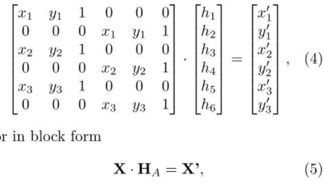
, thus the Equation 1 can be formulated in terms of an inhomogeneous set of linear equations as Equation 4
x1 y1 1 0 0 0 0 0 0 x1 y1 1 x2 y2 1 0 0 0 0 0 0 x2 y2 1 x3 y3 1 0 0 0 0 0 0 x3 y3 1
· h1 h2 h3 h4 h5 h6 = x′ 1 y′ 1 x′ 2 y′ 2 x′ 3 y′ 3 , (4)
or in block form
X·HA=X’, (5)
where xi = £
xi yi¤ and x’i = £
x′ i y′i
¤
are the match pairs of points in inhomogeneous coordi-nates andHA has the form of Equation 6
HA=
h1 h2 h3 h4 h5 h6
0 0 1
. (6)
To estimate HA from 3 matched pairs of pointsxi↔x’i,i= 1,2,3, we can solve the
Equa-tion 5 using the pseudo-inverse as
HA= (XTX)−
1
·XTX’ (7)
whose computation is fast due to the low matrix dimensions.
2.2 Reprojection error
After an affine homography HA has been
com-puted, an error measure can be considered in order to verify whether a given matched pair of points belongs to the plane represented byHA. We use
thereprojection error which can be defined as
ei=|xi−ˆxi|
2
+|x’i−x’ˆi|
2
, (8)
whereˆx’i=HAxandˆxi=H−
1
A x’.
When the reprojection erroreiis below a
cer-tain threshold, we consider that the given matched pairxi↔x’i belongs to the plane represented by
HA.
3 Plane Detection
the set of matched pairs of points from combined Harris detector and SIFT descriptor, we calculate homographies and perform a clustering scheme to detect planes present in the imaged scene.
The entire methodology used is described in the following sections.
3.1 Interest points detection
Different primitives to detect and match image points exist in the literature (Mikolajczyk and Schmid, 2004). The Harris corner detector was chosen since it is fast, reliable and provides good repeatability under varying rotation and illumina-tion. The Harris’ method lies on the calculation of a matrix, M, using the partial derivatives of the intensity function
M =w⊗
³ ∂I ∂x
´2 ³ ∂I ∂x
´
·³∂I ∂y ´
³ ∂I ∂x ´
·³∂I ∂y
´ ³
∂I ∂y
´2
, (9)
wherewspecifies a gaussian window.
A corner is detected thresholding a measure based on the determinant and trace of the matrix M (equation 9).
M =
µ
A C C B
¶
det(M) =AB−C2 trace(M) =A+B
R=det(M)−k(trace(M))2
(10)
where k is constant and empirically adjustable, and R is called by corner response. Points with R above a certain threshold Th are considered a
corner.
In order to eliminate weak corners a non-maximal suppression procedure is performed in the neighborhood of a detected corner.
3.2 Local descriptor
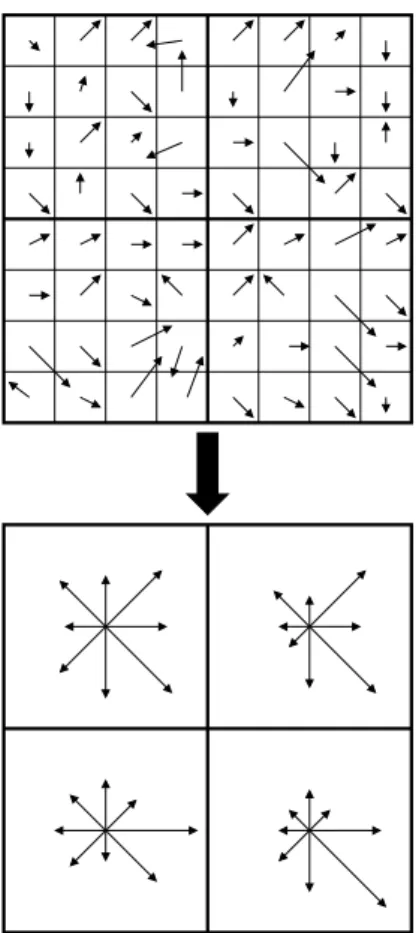
Following the detection of interest points in the two consecutive images, a local descriptor must be used to establish a measure of correlation between the possible candidates to a matched pair of cor-ners. This work uses the Scale Invariant Feature Transform descriptor. The combination of Harris detector with the SIFT descriptor can be consid-ered as a good choice because it produces good and fast results (Mikolajczyk and Schmid, 2005). The SIFT descriptor is a local descriptor highly distinctive and invariant to changes in il-lumination and 3D viewpoint. The descriptor is based on the gradient magnitude and orientation of all pixels in a region around the keypoint. These are weighted by a gaussian window and accumu-lated into orientation histograms summarizing the contents over subregions, as shown in Figure 2.
The length of each arrow corresponds to the sum of the gradient magnitudes near that direction within the region.
Figure 2: This figure shows a 2×2 descriptor array computed from an 8×8 set of samples. Each de-scriptor has 8 bins. The dede-scriptor is represented by a vector of size 32 (2×2×8).
The orientation histogram entries correspond-ing to the lengths of the arrows in the bottom of Figure 2. The descriptor is formed from a vector containing all these entries.
The distance between histograms (SIFT de-scriptor) is used as measure of correlation. A sim-ple Euclidean measure of distance is used. If the distance is below a certain threshold then a pos-sible matched pair is detected.
3.3 Regressive corner filtering and matching
A regressive filtering scheme is used to establish a correspondence between the detected corners and finding matched pairs.
every corner in the second image 2, only the best correlated corner in the first image is maintained. At the end of the filtering, a set of matching pairs of cornersM is obtained from the two images.
Given M, a Delaunay triangulation is per-formed only on the detected corners of the first image. Since the set of triangles has been ob-tained, a clustering scheme must be applied to join triangles in the same plane and discard triangles belonging to virtual planes in the image.
3.4 Clustering points
The clustering scheme used is based on affine ho-mography and reprojection error that allows ob-taining planes and joining points in the same plan. Given the set of matched points M and the set of Delaunay triangles T, we defineHp as the
set of allphomographies existing between the two images. Each homography inHp defines a plane
in the image. Initially Hp is defined as empty.
The first affine homographyHA is computed
us-ing the three points of the first triangleT(1) and their matched pairs into the set M according to the Equation 7. The homography HA obtained
is included inHp, and all used points are marked
asvisited and assigned to the homographyHp(1),
i.e., the first plane.
In the next step, the next triangle of T and their matched points in M is taken. For each Hp(i) inHp, all points of the triangle are verified if
they belong to any of the existing planes inHp. If
the point had been marked asnot-visited and the reprojection error forHiis below a certain
thresh-old, the point is marked asvisitedand assigned to the homographyHi. If the point had been marked
asvisited and if the new reprojection error forHi
is smaller than the old one, the point is assigned to the plane Hi. In the case where all points of
the triangle do not belong to any existing plane, a new affine homography HA is computed with
those points. The new homography represents a new plane and is included inHp. This loop is
per-formed until there are no unvisited matched pairs of points.
The clustering method described before can be presented in the Algorithm 1.
At the end of clustering stage, only planes with a number of points above a certain threshold are considered.
4 Experimental Results
In this section we report experiments that demon-strate accurate plane detection from two consecu-tive frames of an image sequence. Four image se-quences of different outdoor scenes were acquired by a camera. All used images in the experiments are in gray level with size 640×480.
Algorithm 1
1 Create an empty set of homographiesHp
2M: set of matched points between two images 4T: set of triangles of the first image
5t: number of triangles in T 6err: reprojection error
7Te: reprojection error threshold
TakeM andT(1), computeHA and put inHp
Assigned the three points of the triangle T(1) toHp(1), and mark them as visited
forj = 2 :t do
fori = each one inHp do
foreach pointpofT(j)do if p=not-visited then
if err < Tethen
AssignptoHp(i)
Markpasvisited end if
else if p=visited then if err < erroldthen
UpdateptoHp(i)
end if end if end for end for
if AllpofT(j) =not-visited then Compute new HA and put inHp
Assign allpto the newHAand mark them
as visited end if end for
Different parameters were empirically ad-justed at each stage of the entire process of plane detection. The following sections discuss each one of them.
4.1 Interest point detection
At this stage, the Harris detector was imple-mented using k = 0.13 and a gaussian window with standard deviationσ= 1.5 and size of 6σ×
6σ. A threshold valueTh was used to distinguish
between corners and non-corners. Th must be set
high enough to avoid the detection of false corners which may have a relatively large corner response R (Equation 10) due to noise. The value of Th
is based on the maximum corner response com-puted,Rmax. It was usedTh = 0.01·Rmax.
Af-ter all corners had been detected, a non-maximum suppression scheme was performed with a window of size 10×10, in order to eliminate weak corners.
4.2 Local descriptor
of size π/4. The total size of SIFT descriptor is 128 (4×4×8).
A simple Euclidean distance d was used to compare descriptors. If d < Tm then we have a
possible matched pair of interest points. It was initializedTm= 10.
4.3 Regressive corner filtering and matching
In the regressive corner filtering and matching stage, we must perform a search in the second im-age for a corner that best matches a specific corner in the first image. This should be done for all de-tected corners in the first image. The size of the region of search can be constrained to improve the computational efficiency of the algorithm. This re-gion can be defined based on the largest displace-ment of pixel, i.e., based on the camera’s move-ment during the acquisition process. In our case a region around the interest point of size 25×25 was used.
The value ofTmis dynamically adjusted
dur-ing the process of matchdur-ing. When a possible match is found, the value of the thresholdTm is
updated with the computed distanced. This was done to allow that the best candidate is chosen as a match.
4.4 Clustering points
Only one parameter is adjustable at this stage. A reprojection error threshold was empirically cho-sen as Te = 5.0. The value of Te is dynamically
updated during the clustering process. Thus, each matched pair of points in the setM is assigned to the best homography in the setHp based on the
computed reprojection error.
4.5 Results
Four different sequences were used in the exper-iments. Sequences with planes at different posi-tions and orientaposi-tions in the scene were chosen. Figure 3 shows two frames of a sequence.
(a) Frame 01 (b) Frame 02
Figure 3: Two consecutive frames of a sequence used in experiments.
The planes detected are shown using colored markers in the first frame of each sequence. The results for the all sequences are shown in Figures 4, 5, 6 and 7.
Figure 4: Colored markers specify the detected planes.
Figure 5: Colored markers specify the detected planes.
4.6 Discussion
The sequences were acquired under different con-ditions of illumination and different positions of the camera relative to the planes in the scene. The best results were obtained using Harris corner de-tector combined with SIFT descriptor.
The matching process is one of the most im-portant stages of the algorithm. An imim-portant pa-rameter is the size of the region in which a match is searched for.
Each one of the four sequences presents two major planes of a scene. The results clearly show that the algorithm performs well using outdoor images.
5 Conclusion
Figure 6: Colored markers specify the detected planes.
Figure 7: Colored markers specify the detected planes.
Future work will be concentrated at joining affine homography and affine optical flow to im-prove the precision and reliability under a wide range of conditions.
References
Agarwal, A., Jawahar, C. V. and Narayanan, P. J. (2005). A survey of planar homogra-phy estimation techniques, Technical Report IIIT/TR/2005/12, Centre for Visual Infor-mation Technology.
Harris, C. and Stephens, M. (1988). A combined corner and edge detection,Proceedings of The Fourth Alvey Vision Conference, pp. 147– 152.
Hartley, R. and Zisserman, A. (2004). Multiple View Geometry in Computer Vision, second edn, Cambridge University Press.
Lowe, D. (2003). Distinctive image features from scale-invariant keypoints,International Jour-nal of Computer Vision, Vol. 20, pp. 91–110.
Mikolajczyk, K. and Schmid, C. (2004). Scale and affine invariant interest point detectors,
International Journal of Computer Vision 60(1): 63–86.
Mikolajczyk, K. and Schmid, C. (2005). A perfor-mance evaluation of local descriptors, IEEE Transactions on Pattern Analysis & Machine Intelligence27(10): 1615–1630.
Okada, K., Kagami, S., Inaba, M. and Inoue, H. (2001). Plane segment finder: Algorithm, implementation and applications, IEEE In-ternational Conference on Robotics and Au-tomation, Vol. 2, IEEE Computer Society, pp. 2120–2125.
Piazzi, J. and Prattichizzo, D. (2006). Plane de-tection with stereo images, IEEE Interna-tional Conference on Robotics and Automa-tion, IEEE Computer Society, pp. 922–927.
Rodrigo, R., Chen, Z. and Samarabandu, J. (2006). Feature motion for monocular robot navigation, Information and Automation, 2006. ICIA 2006. International Conference on, pp. 201–205.
Silveira, G., Malis, E. and Rives, P. (2006). Real-time robust detection of planar regions in a pair of images, International Conference on Intelligent Robots and Systems, IEEE Com-puter Society, pp. 49–54.