Explore the Performance of the ARM
Processor
Using JPEG
N.N. Ganvir, A.D. Jadhav SCOE, Pune
Abstract: Recently, the evolution of embedded systems has shown a strong trend towards application- specific, single- chip solutions. The ARM processor core is a leading RISC processor architecture in the embedded domain. The ARM family of processors supports a unique feature of code size reduction. In this paper it is illustrated using an embedded platform trying to design an image encoder, more specifically a JPEG encoder using ARM7TDMI processor. Here gray scale image is used and it is coded by using keil software and same procedure is repeated by using MATLAB software for compare the results with standard one. Successfully putting a new application of JPEG on ARM7 processor.
I. INTRODUCTION
Real-time embedded systems are a challenge to implement. An embedded environment constrains the energy consumption, the memory space, and the execution time of an application. On the other hand, the complexity of the applications running on an embedded platform keeps increasing. Examples include next-generation cell phones, portable game-boys and digital assistants, smartcards, and medical monitoring devices.
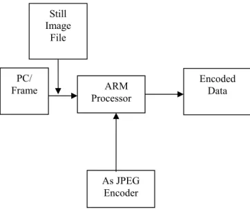
Figure 1. Generalized Block Diagram
Looking forward to new era of image processing, modernized and fastest ways to
compress the images by using JPEG , in the world of photography and its best outputs in terms of image compression ,world is definitely in need of new approaches. To achieve this we need to evaluate the performance of ARM PROCESSOR by using JPEG as one of the application. This is an embedded approach for the compression which can be useful and suitable for the application like digital camera. Now a days Digital camera has become fastest and best means in the world of photography, and so as the images created by it. Figure 1 shows generalized block diagram of ARM based JPEG encoder. As any Images file created by digital is to be compressed by using JPEG standard and then further this file will be processed through serial communication by using ARM processor. JPEG acts as a JPEG encoder for the ARM processor. In this paper, evaluating the performance of ARM processor family with JPEG. Here, image file is taken from windows and then converted into grayscale image by using MATLAB then is process through ARM.
II. ARMPROCESSOR
An Embedded Processors is simply a micro Processors that has been “Embedded” into a device. It is software programmable but interacts with different pieces of hardware. The three most important design criteria for embedded processors are performance, power, and cost. Performance is a function of the parallelism, instruction encoding efficiency, and cycle time. Power is approximately a function of the voltage, area, and switching frequency also a function of execution time. cost is a function of both area (how many fit on a die) and the complexity of use (in terms of engineering cost).ARM seems to be leading the way in this field of processing. The processor has found this as one of its greatest markets, mainly because of the steps the company has taken to fit into the embedded market and the architecture it has adopted. Other embedded applications that take advantage of such processors are: disc drive controllers, automotive engine control and management systems, digital auto surround sound, TV-top boxes and internet appliances. Other products are still being modified to take advantage of it: toys, watches, etc. The possible applications are almost endless. ARM can offer low cost, high performance and low power consumption, each of which is required to make a ARM
Processor
Encoded Data
As JPEG Encoder PC/
Frame Still Image
portable embedded item marketable in today's world. Not to mention the fact that a whole sub-group of ARM architecture has been dedicated to function strictly to signal processors.
2.1 FEATURES OF ARM PROCESSOR
FOLLOWING ARE THE FEATURES OF THE ARM
PROCESSOR.
a) On-chip integrated oscillator operates with external crystal in range of 1 MHz to30 MHz or with external oscillator from 1 MHz to 50 MHz.
b) Power saving modes include idle and Power-down.
c) Individual enable/disable of peripheral functions as well as peripheral clock scaling down for additional power optimization. d) Two 32-bit timers/external event counters
(with four captures and four compare channels each), PWM unit (six outputs) and watchdog.
e) Low power Real-time clock with independent power and dedicated 32 kHz clock input. f) Multiple serial interfaces including two
UARTs (16C550), two Fast I2C (400 kbit/s), SPI™ and SSP with buffering and variable data length capabilities
g) Vectored interrupt controller with configurable priorities and vector addresses. h) Up to 47 of 5 V tolerant general purpose I/O
pins in tiny LQFP64 package.
i) Processor wake-up from Power-down mode via external interrupt or Real-time Clock. j) Single power supply chip with Power-On
Reset (POR) and Brown-Out Detection (BOD) circuits:– CPU operating voltage range of 3.0 V to 3.6 V (3.3 V ± 10 %) with 5 V tolerant I/O pads.
III. JOINT PHOTOGRAPHYEXPERT GROUPS
For the past few years, a joint ISO/CCITT committee known as JPEG (Joint- Photographic Experts Group) has been working to establish the first international compression standard for continuous tone still images, both grayscale and color. JPEG’s proposed standard aims to be generic, to support a wide variety of applications for continuous tone images. To meet the differing needs of many applications, the JPEG standard includes two basic compression methods, each with various modes of operation. A DCT based method is specified for “lossy’’ compression, and a predictive method for “lossless’’ compression. JPEG features a simple lossy technique known as the Baseline method, a subset of the other DCT based modes of operation. The Baseline method has been by far the most widely implemented JPEG method to date, and is sufficient in its own right for a large number
of applications. JPEG has following modes of operation:
Sequential encoding: each image component is encoded in a single left to right top to bottom scan.
Progressive encoding: the image is encoded in multiple scans for applications in which transmission time is long, and the viewer prefers to watch the image build up in multiple coarse to clear passes.
c) Lossless encoding: the image is encoded to guarantee exact recovery of every source image sample value (even though the result is low compression compared to the lossy modes).
d) Hierarchical encoding: the image is encoded at multiple resolutions so that lower resolution versions may be accessed without first having to decompress the image at its full resolution.
3.1 BLOCK DIAGRAM DESCRIPTION OF JPEG
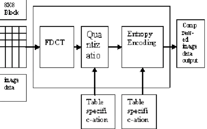
Figure2 shows the key processing steps which are the heart of the DCT Based modes of operation. These figures illustrate the special case of Single component (grayscale) image compression. Color image compression can then be approximately regarded as compression of multiple grayscale images, which are either compressed entirely one at a time, or are compressed by alternately interleaving 8x8 sample blocks from each in turn. For DCT sequential mode codecs, which include the Baseline sequential codec, the simplified diagrams indicate how, single component compression works in a fairly complete way. Each 8x8 block is input, makes its way through each processing step, and yields output in compressed form into the data stream.
Figure 2. DCT Based Encoder Processing Steps 8 X 8 DCT
remaining 63 coefficients are called the “AC coefficients.’’ . Figure 4 shows that DCT operation and related equation. For ARM Processor, Floating-point arithmetic is a more flexible and general Mechanism than fixed-point. With floating-point, system designers have access to wider dynamic range (the ratio between the largest and smallest numbers that can be represented). As a result, floating-point are generally easier to program than their fixed point but usually are also more expensive and have higher power consumption. The increased cost and power consumption result from the more complex circuitry required within the floating-point which implies a larger silicon die.
F(I,j) f(u,v)
Figure 3. Spatial domain to frequency domain
N-1 N-1
C(u,v) = α (u)α(v) ∑ ∑ f (x,y) cos [π (2x+1)u ]cos[π (2y+1)v ] - - -(1.4)
x=0 y=0 2 N 2 N
Figure 4. Sample bmp image 8X8
Fig 4 shows the sample 8X8 bmp image, here image is somewhat expanded so tat clear image can be seen. This image has some color coefficients, first converting this color coefficient into gray scale by using command from MATLAB gray2ind converting all color components into gray coefficients table 1 shows image coefficients and table 2 shows gray image coefficients.
TABLE I. SAMPLE IMAGE COEFFICIENTS
255 255 255 255 255 255 255 255 255 255 255 255 255 255 255 255 255 255 0 0 0 0 255 255 255 255 0 0 0 0 255 255 255 255 0 0 0 0 255 255 255 255 0 0 0 0 255 255 255 255 255 255 0 0 255 255 255 255 255 255 255 255 255 255
TABLE II. CONVERTING ALL COLOR COEFFICIENTS INTO GRAY
15 15 15 15 15 15 15 15 15 15 15 15 15 15 15 15 15 15 0 0 0 0 15 15 15 15 0 0 0 0 15 15 15 15 0 0 0 0 15 15 15 15 0 0 0 0 15 15 15 15 15 15 0 0 15 15 15 15 15 15 15 15 15 15
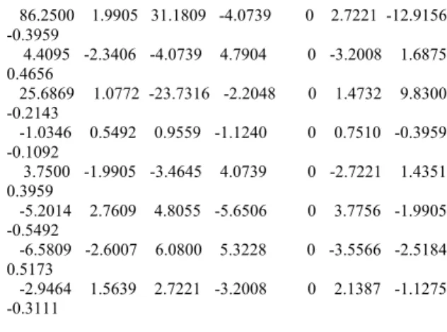
These coefficients are directly used in Keil software for embedded version. Since we can use JTAG for this but it increases C code, so directly taking image coefficients to process for DCT. Table 3 shows DCT values for sample image and its is perfectly matched with ARM. This DCT code is written as per R [1]. In ‘C’ code all the last values are get divided by 65535 because when we are converting sample image into gray we are using index 16 and in MATLAB it is index 16 is for 65535.
TABLE III. DCT RESULT FOR SAMPLE IMAGE.
86.2500 1.9905 31.1809 -4.0739 0 2.7221 -12.9156 -0.3959
4.4095 -2.3406 -4.0739 4.7904 0 -3.2008 1.6875 0.4656
25.6869 1.0772 -23.7316 -2.2048 0 1.4732 9.8300 -0.2143
-1.0346 0.5492 0.9559 -1.1240 0 0.7510 -0.3959 -0.1092
3.7500 -1.9905 -3.4645 4.0739 0 -2.7221 1.4351 0.3959
-5.2014 2.7609 4.8055 -5.6506 0 3.7756 -1.9905 -0.5492
-6.5809 -2.6007 6.0800 5.3228 0 -3.5566 -2.5184 0.5173
-2.9464 1.5639 2.7221 -3.2008 0 2.1387 -1.1275 -0.3111
3.2 Quantization
F‘ [u, v] = round (F [u, v] / q [u, v]). Why? -- To reduce number of bits per sample Example: 101101 = 45 (6 bits).
Q [u, v] = 4 --> Truncate to 4 bits: 1011 = 11. For the ARM Processor, we are quantizing File i.e. reducing file size length. Memory required, execution time, speed required will be less for this block. Here four table specifications are required for quantization. Each table has 64 byte, so total 256 bytes are required. For quantization Luminous table for color image is used because it is same for gray image. Table 4 shows quantization table for gray scale image and Table 5 shows keil output of quantization and it is again is perfectly matched with MATLAB.
TABLE IV. QUANTIZATION TABLE USED FOR GRAY SCALE IMAGE.
Quant= [16 11 10 16 24 40 51 61; 12 12 14 19 26 58 60 55; 14 13 16 24 40 57 69 56; 14 17 22 29 51 87 80 62; 18 22 37 56 68 109 103 77; 24 35 55 64 81 104 113 92; 49 64 78 87 103 121 120 101; 72 92 95 98 112 100 103 99]. Equation for quantization is as follows:
Q=DCT (x,y) /quant. ---- (1.5) TABLE V. OUTPUT OF KEIL FOR QUANTIZATION
11.5530 -12.8668 10.8411 -6.1552 -20.2332 -26.2163 71.2116 -34.8024
0.2988 -0.4504 0.8666 -0.7943 0.4546 -0.9377 1.0041 -0.4286
0.2956 -0.8732 3.9475 -1.5304 0.5620 -4.3798 4.0433 -1.4656
0.0701 0.1057 0.2033 0.1864 0.1067 0.2200 -0.2356 0.1006
0.2541 -0.3830 0.7370 -0.6755 0.3866 -0.7974 0.8539 -0.3645
0.3525 0.5312 1.0222 0.9369 0.5363 1.1061 -1.1844 0.5056
0.1526 0.0529 0.8374 0.0972 0.1857 0.9510 -0.7505 0.2125
0.1997 0.3009 0.5790 0.5307 0.3038 0.6265 -0.6709 0.2864
Here, all the results of DCT and quantization of Keil and MATLAB are perfectly matched. Here, we have used MATLAB only for verification of keil output. Since, algorithm used for JPEG for embedded platform should be matched with standard tool that’s why we have used MATLAB. Up to quantization we can see the output of the image after that image coefficients are scanned or prepared for entropy encoding. Fig 5 shows quantized output and image size.
Sample image file Quantized image file
1.1.KB 368 bytes
Figure 5. Quantized output
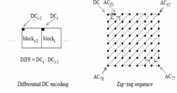
3.3 DC Coding and Zig -Zag Sequence After quantization, the DC coefficient is treated separately from the 63 AC coefficients. The DC coefficient is a measure of the average value of the 64 image samples. Because there is usually strong correlation between the DC coefficients of adjacent 8x8 blocks, the quantized DC coefficient is encoded as the difference from the DC term of the previous block in the encoding order. Figure 6 shows zigzag scanning of an image.
Figure 6. Preparation of Quantized Coefficients for Entropy Coding
All of the quantized coefficients are ordered into the “zigzag” sequence. This ordering helps to facilitate entropy coding by placing low frequency coefficients (which are more likely to be non zero) before high frequency coefficients.Here,2D to 1D is converted and then again it is converted image coefficients are same but is zig-zag sanned.
3.4 Entropy Coding
image are needed to decompress it. Huffman tables may be predefined and used within an application as defaults, or computed specifically for a given image in an initial statistics gathering. Pass prior to compression. Such choices are the business of the applications which use JPEG; the JPEG proposal specifies no required Huffman tables. Huffman table needs 64 bytes for encoder and 64 bytes for decoder. Table specification is different for color and grayscale image. The final image and output after zig-zag is as shown in fig3.10 and 3.11. Fig3.10 shows the output of zig-zag scanning its values are fixed to near zero by suing MATLAB n same id done with the help of keil embedded software. Fig 3.11 shows output codeword of sample image.For keil we have to intialize serial port and through hyper terminal output is shown.fig 7 shows that out of 64 coefficients 47 coefficients are zeros,hence image is successfully compressed because we are using JPEG lossy mode.
TABLE VI. OUTPUT OF ZIG-ZAG SCANNING.
11 -12 10 -6 -20 -26 71 -34 0 0 0 0 0 0 1 0 0 0 3 -1 0 -4 4 -1 0 0 0 0 0 0 0 0 0 0 0 0 0 0 0 0 0 0 -1 0 0 1 -1 0 0 0 0 0 0 0 0 0 0 0 0 0 0 0 0 0
1*01000*01000*01000*01000*01000*01000*010 00*01000*01000*100*01000*01000*01000*
Figure 7. Huffman codeword output of hyper terminal.
IV. SELECTION OF THE ARM7TDMI PROCESSOR
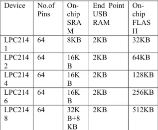
Table1 shows comparison of ARM&TDMI family. Device No.of Pins On-chip SRA M End Point USB RAM On-chip FLAS H LPC214 1
64 8KB 2KB 32KB
LPC214 2 64 16K B 2KB 64KB LPC214 4 64 16K B 2KB 128KB LPC214 6 64 16K B 2KB 256KB LPC214 8 64 32K B+8 KB 2KB 512KB
Table 1:Device Information of ARM Processor
LPC2148 has 32KB in addition with 8KB memory and 512KB on chip FLASH memory. So selecting LPC2148 for future work related to color images. Conclusion
JPEG is not the application of ARM7 processor since this processor is not in the area of image compression. In this work, after successful experimentation on JPEG lossy technique, code word is obtained using Huffman coding. Outcome of this work shows that code word is generated by scanning quantization matrix. Using this technique, JPEG lossy technique is successfully implemented on keil platform to assert the Uart signal of LPC2148 processor, so as to show the output on hyper terminal. Image compression is nearly about 90% to 95%.
References:
[1] www.Xillinx.com
[2] Gunnar Braun , Achim Nohl, Andreas Weiferink ,”Processor/ Memory Co-Exploration on Multiple Abstraction Levels”,IEEE 2003
[3] Gregory K. Wallace,”The JPEG Still Picture Compression Standard”, IEEE 1991
[4] Ieeexplore.ieee.org/ie15/8483/26600/01253730.pdf. [5] CHANG-AN TASI,LAN –DA VAN ,”ARM BASED
SOC PROTOTYPING PLATFORM USING APTIX “,IEEE 5 MARCH 2005
[6] Bart Weuts, “Software for ARM Processors and AMBA Methodology-based Systems”, Volume 3, Number 4, 2004 [7] J,Weinberger and Gadiel Seroussi,” lossless Image
compression Algorithm principles and standardization. The loco –I into JPEG-LS “.
[8] For MATLAB investigation
http://www.stanford.edu/class/ee 68b/Prrojects/jcsabat/Mcpperf.html
[9] Jike Chong , Abhijit Dawore, Kelvin Lwi,” Concurrent embedded design for multimedia:JPEG encoding on xillinx FPGA”,EECS,April 16,2006
[10] www.cs.vcsd.edu/classes/spo2/cse29/-
e/slides/armlect.pdf.
[11] Krishna swami ,Gupta,” Profile guided selection of ARM and THUMB instruction”2002.
[12] Rishi Bhardwaj, Phillip Reames, Russell Greenspan Vijay Srinivas Nori, Ercan Ucan”A Choices Hypervisor on the ARM architecture”,2003
[13] Diego Santa-Cruz and Touradj Ebrahimi,” AN ANALYTICAL STUDY OF JPEG 2000 FUNCTIONALITIES”, IEEE. 2000
[14] Kai-Yuan Jan*, Chih-Bin Fan, An-Chao Kuo, Wen-Chi Yen and Youn-Long Lin,”A platform based SOC design methodology and its application in image compression”, Int. J. Embedded Systems, Vol. 1, Nos. 1/2, 2005 23 [15] Yu-Lun Huang and Jwu-Sheng Hu,” A Teaching
Laboratory and Course Programs for Embedded Software Design”, iCEER-2005
[16] Hany Farid,” Digital Image Ballistics from JPEG Quantization”, TR2006-583.
[17] JPEG Technical Specification, Adobe Developer Support year1992.
[18] “INFORMATION TECHNOLOGY JPEG 2000 IMAGE CODING SYSTEM”,JPEG 2000 FINAL COMMITTEE DRAFT VERSION 1.0, 16 MARCH 2000.
[19] Michael D. Adams and Faouzi Kossentini,” JasPer: A Software-Based JPEG-2000 Codec Implementation”.
CONTINUOUS-TONE STILL IMAGES”, REQUIREMENTS AND GUIDELINES, CCITT Rec T.81.