An Application of Best L1 Piecewise Monotonic Data Approximation to Signal Restoration

An Application of Best

_L

₁

Piecewise Monotonic

Data Approximation to Signal Restoration

I. C. Demetriou

Abstract—We consider an application of the bestL1piecewise monotonic data approximation method to univariate signal restoration. We extend numerical examples concerned with the L2 analogous method to theL1 case and we show the efficacy of a relevant software package that implements the method in data fitting and in denoising data from a medical image. The piecewise monotonic approximation method makes the smallest change to the data such that the first differences of the smoothed data change sign a prescribed number of times. Our results exhibit some strengths and certain advantages of the method. Therefore, they may be helpful to the development of new algorithms that are suitable to signal restoration calculations.

Index Terms—absolute value, data smoothing, divided dif-ferences, L1-norm, piecewise monotonic approximation, signal restoration

I. INTRODUCTION

L

of a signalφ(x)measured at the abscissae x1< x2< · · · < xn, but these measurements include errors and the

data are to be used to provide a restoration to φ(x). Most methods of data approximation assume that measurements of function values can be approximated by a form that depends on relatively few parameters. Spline functions, for instance, are candidates for approximation, but sometimes it is difficult to choose a suitable one. Therefore, Demetriou and Powell [10] take the view that some useful smoothing should be possible if the data fail to possess a property that is usually obtained by the underlying function. They assume that if the signal has turning points, then the number of measurements is substantially greater than the number of turning points. Therefore they propose algorithms that modify the measurements if their first differences{yi+1−yi:

i= 1, . . . , n−1} include more thank−1 sign changes, a condition which allowskmonotonic sections to the smoothed data, where k is a prescribed positive integer. In [10] (best

L2 approximation), thek−1optimal turning points and the least sum of squares change to the data are computed in

O(n2

+knlogn)computer operations. The important result in this work is the substantial reduction of the number of data that need be considered in finding the optimal turning points, among O(nk_{) combinations of possible combinations of}

turning points. The special casesk= 1,2are solved in only

O(n)operations. Applications of the method in spectroscopy, signal restoration and image processing are presented by [4], [16], [26]) and references therein. For general references in signal and image processing see [21] and [13].

In [7], piecewise monotonic data approximation is studied in the sense of the least sum of the moduli of the errors (best

Manuscript received October 31, 2013.

I. C. Demetriou is with the Department of Economics, Univer-sity of Athens, 8 Pesmazoglou street, Athens 10559, Greece (e-mail: demetri@econ.uoa.gr).

L1 approximation). In general, a bestL1approximation has the remarkable property, which makes it particularly suitable to data smoothing when there are few gross errors in the data, that the magnitudes of the errors make no difference to the best fit (see, for example, [20]). The main result of [7] is that a bestL1calculation, as the corresponding L2one, can be decomposed into optimal monotonic calculations between adjacent turning points. L1PMA is the Fortran software package that the author has developed [8] to implement the method of [7] with certain extensions that improve efficiency. L1PMA calculates a best L1 fit with at most k monotonic sections of the data in O(n3_+kn2₎

computer operations. This complexity reduces to O(n2₎

when k = 1 or k = 2. The software package has been tested on a variety of data sets showing in practice quadratic performance with respect ton. The package employs techniques for calculating the median and the best L1 monotonic approximation (k = 1), which is an integral part of the package. The monotonic problem during the last 60 years has received considerable attention in various fields, including engineering, economics, operations research and statistics.

Some advantages that are gained by employing the piece-wise monotonic constraints to data approximation are as follows. We avoid the assumption thatφ(x)has a form that depends of a few parameters, which occurs in many other approximation techniques, as for example, in splines [3] and wavelets [14]; the smoothing process is a projection because, if it is applied to the smoothed data, then no changes are made to; piecewise monotonicity is a property that occurs in a wide range of underlying functions; any degree of undulation of the data can be accommodated. Moreover, the piecewise monotonic approximation method is particularly suitable when the data errors are large and uncorrelated.

This paper is concerned with an application of the best

L1 piecewise monotonic data approximation method [8] to univariate signal restoration. It presents a survey of the method and extends some numerical examples from least squares piecewise monotonic data approximation [9] to the

L1case. There are many similarities as well as considerable differences between these methods.

II. BESTL1PIECEWISEMONOTONICDATA APPROXIMATION

We regard the measurements as components{φi=φ(xi) :

i= 1,2, . . . , n} of an−vector φ. The user providesk and specifies whether the first monotonic section is increasing or decreasing. Then the method of [7] automatically derives the optimal turning points and the best L1 fit. Specifically, the method calculates a vectory that minimizes the sum of the moduli of the errors

Φ(y) =

n

X

i=1

|yi−φi| (1)

subject to the piecewise monotonicity constraints

ytj−1 ≤ytj−1+1≤ · · · ≤ytj, if j is odd

ytj−1 ≥ytj−1+1≥ · · · ≥ytj, if j is even

)

, (2) where the integers {tj : j = 0,1, . . . , k}, namely the

positions of the turning points or extrema of the fit, satisfy the conditions

1 =t0≤t1≤ · · · ≤tk=n. (3)

Since the integers {tj:j= 1,2, . . . , k−1} are variables

in the optimization calculation that gives a best L1 fit, the number of combinations of integer variables is raised to the orderO(nk_{), which makes non practicable to investigate all}

these combinations individually for optimality. Fortunately the piecewise monotonic approximation problem has a rich structure that allows an efficient calculation of an optimal fit. To begin with, the constraints prevent the equation y =

φ, because ifφdoes not satisfy the piecewise monotonicity constraints, then {tj :j = 1,2, . . . , k−1} are all different.

Moreover, the optimal value of ytj is independent of the components {yi : i 6= tj}, which gives the interpolation

conditions

ytj =φtj, j= 1,2, . . . , k−1. (4) The most important property, however, is that each mono-tonic section in a best L1 piecewise monotonic fit is an optimal fit itself to the corresponding data, so it can be obtained by a separate calculation. Indeed, the components {yi:i=tj−1, tj−1+ 1, . . . , tj}on[xtj−1, xtj]minimize the sum of the moduli

tj

X

i=tj−1

|yi−φi| (5)

subject to the constraints

yi≤yi+1, i=tj−1, . . . , tj−1, if j is odd (6)

or subject to the constraints

yi≥yi+1, i=tj−1, . . . , tj−1, ifj is even. (7)

In the former case the sequence {yi : i = tj−1, tj−1 +

1, . . . , tj} is a best L1 monotonic increasing fit to {φi :

i = tj−1, tj−1+ 1, . . . , tj} and on the latter case a best

L1 monotonic decreasing one. Therefore, provided that{ti:

i = 1,2, . . . , k−1} are known, the components of y can be generated by solving a separate monotonic problem on each section [xtj−1, xtj]. The problem with the decreasing monotonicity constraints may be treated computationally as

the problem with the increasing monotonicity constraints after reversing the order of the data. We introduce the notation α(tj−1, tj) and β(tj−1, tj) for the least value of

(5) subject to the constraints (6) and (7) respectively. We denote by δ(k, n) the least value of (1) at the required minimum and, ifkis odd, we obtain the expressionδ(k, n) =

α(t0, t1) + β(t1, t2) +α(t2, t3) + · · · + α(tk−1, tk) and

analogously if k is even, where we replace the last term in this sum byβ(tk−1, tk).

The problem of minimizing (5) subject to (6) is a linear programming problem that need not have a unique solution (see [11], [12], [18] for general references and methods on L1 approximation and linear programming). Although it is usual to calculate the solution of a L1 approximation problem by applying linear programming techniques (see, [1], [2]), we have developed a method that is faster than a general linear programming calculation. Specifically, the calculation of a best monotonically increasing approximation to φ seeks intervals where its components have different constant values. In the L1 case these values are equal to the median of the corresponding data points, while in the

L2case they are equal to their mean value. The intervals are formed by using the remarkable property that any constraints which are satisfied as equalities by a bestL1approximation subject to a subset of the monotonicity constraints are also satisfied as equalities by a bestL1 approximation subject to all monotonicity constraints (6). The consideration of [5] that the specific value of the median should be chosen carefully in order that the finalysatisfy the constraints (6) has been taken into account in the development of Algorithm 2 of [8] that performs the calculation of a bestL1 monotonic increasing fit on[xtj−1, xtj] together with all the numbers

α(tj−1, t) =

t

X

i=tj−1

|yi−φi|, t=tj−1, . . . , tj (8)

inO((tj−tj−1)2)computer operations. General algorithms for the bestL1monotonic increasing approximation problem are given by [17], [22] and [24].

Further, it is proved that an optimal fity associated with the integer variables {tj : j = 1,2, . . . , k−1} can split at

tk−1into two optimal sections. One section that provides an optimal fit on[x1, xtk−1], which in fact is similar toy with one monotonic section less, and one section on [xtk−1, xn] that is a single bestL1 monotonic fit to the remaining data. Therefore with the initial values

δ(1, t) =α(t0, t), for t= 1,2, . . . , n, (9) the optimization problem can be expressed in terms of the dynamic programming formula

δ(r, t) = min

1≤s≤t[δ(r−1, s) +α(s, t)], ifr is odd (10)

or

δ(r, t) = min

1≤s≤t[δ(r−1, s) +α(s, t)], if ris even, (11)

where 1 ≤ t ≤ n. The implementation of these formulae includes several options that are considered by [10] and [7]. Demetriou [8], especially, has implemented this method in Fortran and provided a software package that derives a solution in O(n2

m+km2

is the number of local extrema of the data. For example, an integer p is the index of a local maximum of the sequence

φi, i = 2, . . . , n−1 if φp−1 ≤ φp and φp > φp+1, and similarly for a local minimum. Since m is a fraction of n, the complexity of the formulae (10) and (11) is reduced at least be a factor of 4. Further, it is stated in [8] that as more data are inserted into the calculation, that is as

n increases for a fixed k, or as the number of monotonic sections increases by 2 for a fixedn, the rightmost extremum of the associated optimal approximation increases as well. The reported numerical results [8] show that increasing k

beyond 3 either has a small effect in the computation times or no effect at all. Indeed, as kincreases, the ranges where the monotonic algorithm is applied are decreased due to the increasing property of the rightmost extremum. We see that the complexity of the piecewise monotonic approximation method is dominated by the term n2_m

, but in practice the mentioned properties restrict considerably the range of s

in the minimization formulae (10) and (11) and make the calculation very efficient.

The method that gives a piecewise monotonic approxima-tion may also be applied to the problem where inequalities (2) are replaced by the reversed ones, in which case the first section of the fit is decreasing. The latter problem may be treated computationally as the former one after an overall change of sign ofφ.

III. NUMERICALEXAMPLES INSIGNALRESTORATION WITHPIECEWISEMONOTONICITYCONSTRAINTS ANDL1

OPTIMALITY

To illustrate the efficacy of the method in signal restoration we present calculations from two numerical examples that are taken from [9]. In addition, the reader will be able to compare the results of the least squares case of [9] with those of this paper. We shall see that the results are very similar.

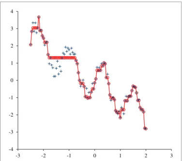
The first example is a best fit with k = 6 monotonic sections ton= 100measurements of the function

φ(x) =sin(5x)−x (12) at equally spaced abscissae in the interval[−2.5,2]. The mea-surements were generated by adding uniformly distributed random numbers from the interval(−0.5,0.5)to the function values φ(xi), i = 1,2, . . . , n. The data are presented in

the second and the third column of Table I, although the abscissae are irrelevant to this calculation. Without any preliminary analysis, the data were fed to L1PMA, six mono-tonic sections were required and the solution was reached immediately in a common pc. The best L1 fit is presented in the fourth column of Table I and the analogous best L2 fit is presented in the fifth column (the L2 fit is obtained as described in [9]); the horizontal lines indicate the turning point positions in either case. Fig. 1 shows the data and the best L1 fit; the data are denoted by (+), the best fit by (o) and the piecewise linear interpolant to the smoothed values illustrates the fit.

The first attempt at fitting the data, on the purpose of demonstrating some features of the piecewise monotonic fit, was not entirely satisfactory. Indeed, the turning points of the fit are at the abscissae x8, x50, x64, x78 and x89, satisfying the interpolation conditions (4). The components

-4 -3 -2 -1 0 1 2 3 4

-3 -2 -1 0 1 2 3

Fig. 1. Graphical representation of the data given in Table I. The data of column 2 annotate the x-axis. The data of column 3 are denoted by (+) and the bestL₁fit of column 4 by (o). The solid line illustrates the fit.

-3 -2 -1 0 1 2 3 4

-3 -2 -1 0 1 2 3

Fig. 2. BestL₁fit (solid line) withk= 8_{monotonic sections to}n= 200

measurements (+) of function (12) produced as described in Section III.

of a best fit consist of ranges of constant values, each such value being the median of the corresponding data within a range. Of course, the monotonic algorithm finds the median of any data values that are needed to achieve monotonicity. For example, we see in the fourth column of Table I that the components of an optimal fit that is obtained by minimizing the function P7

i=3|yi −φi| subject to the

constraintsy3 ≤y4 ≤y5 ≤y6 ≤y7 have the values y3 =

y4 =y5 = y6 = y7 = 3.042, where 3.042 is the (unique) median of the data {3.339,2.852,3.333,2.765,3.042}. The analogous L2 values (fifth column) are y3 = y4 = y5 =

y6 = y7 = ( P7

i=3φi)/5 = 3.066 and are obtained by

minimizing the function P7

i=3(yi − φi)2 subject to the

TABLE I

BEST FITS WITHk= 6_ANDk= 8_{MONOTONIC SECTIONS TO MEASUREMENTS OF FUNCTION(12)}

Best Fit k=6 Best Fit k=8 Best Fit k=6 Best Fit k=8 xi φi yi(L1) yi (L2) yi (L1) yi (L2) xi φi yi(L1) yi (L2) yi (L1) yi (L2)

1 –2.50 2.066 2.066 2.066 2.066 2.066 51 –0.23 –0.710 –0.999 –0.855 –0.999 –0.855 2 –2.45 2.839 2.839 2.839 2.839 2.839 52 –0.18 –0.999 –0.999 –0.855 –0.999 –0.855 3 –2.41 3.339 3.042 3.066 3.042 3.066 53 –0.14 –0.678 –0.678 –0.678 –0.678 –0.678 4 –2.36 2.852 3.042 3.066 3.042 3.066 54 –0.09 –0.186 –0.494 –0.340 –0.494 –0.340 5 –2.32 3.333 3.042 3.066 3.042 3.066 55 –0.05 –0.494 –0.494 –0.340 –0.494 –0.340 6 –2.27 2.765 3.042 3.066 3.042 3.066 56 0.00 –0.146 –0.146 –0.146 –0.146 –0.146 7 –2.23 3.042 3.042 3.066 3.042 3.066 57 0.05 0.086 0.086 0.086 0.086 0.086 8 –2.18 3.673 3.673 3.673 3.673 3.673 58 0.09 0.756 0.583 0.659 0.583 0.659 9 –2.14 2.884 2.884 2.899 2.884 2.899 59 0.14 0.561 0.583 0.659 0.583 0.659 10 –2.09 2.914 2.884 2.899 2.884 2.899 60 0.18 0.735 0.583 0.659 0.583 0.659 11 –2.05 2.584 2.584 2.584 2.584 2.584 61 0.23 0.583 0.583 0.659 0.583 0.659 12 –2.00 2.442 2.442 2.442 2.442 2.442 62 0.27 0.974 0.843 0.908 0.843 0.908 13 –1.95 2.046 2.203 2.157 2.203 2.157 63 0.32 0.843 0.843 0.908 0.843 0.908 14 –1.91 2.203 2.203 2.157 2.203 2.157 64 0.36 1.020 1.020 1.020 1.020 1.020 15 –1.86 2.221 2.203 2.157 2.203 2.157 65 0.41 0.960 0.960 0.960 0.960 0.960 16 –1.82 1.491 1.491 1.491 1.491 1.491 66 0.45 0.161 0.161 0.261 0.161 0.261 17 –1.77 0.962 1.311 1.198 0.962 1.136 67 0.50 0.362 0.161 0.261 0.161 0.261 18 –1.73 1.311 1.311 1.198 0.962 1.136 68 0.55 –0.195 –0.195 –0.195 –0.195 –0.195 19 –1.68 0.886 1.311 1.198 0.886 0.886 69 0.59 –0.848 –0.848 –0.848 –0.848 –0.848 20 –1.64 0.728 1.311 1.198 0.728 0.728 70 0.64 –1.157 –1.025 –1.057 –1.025 –1.057 21 –1.59 0.227 1.311 1.198 0.227 0.227 71 0.68 –1.025 –1.025 –1.057 –1.025 –1.057 22 –1.55 0.236 1.311 1.198 0.236 0.236 72 0.73 –0.989 –1.025 –1.057 –1.025 –1.057 23 –1.50 0.700 1.311 1.198 0.700 0.700 73 0.77 –1.127 –1.127 –1.127 –1.127 –1.127 24 –1.45 1.114 1.311 1.198 0.700 0.704 74 0.82 –1.753 –1.753 –1.753 –1.753 –1.753 25 –1.41 0.369 1.311 1.198 0.700 0.704 75 0.86 –1.855 –1.855 –1.855 –1.855 –1.855 26 –1.36 0.805 1.311 1.198 0.700 0.704 76 0.91 –1.951 –1.855 –1.876 –1.855 –1.876 27 –1.32 0.527 1.311 1.198 0.700 0.704 77 0.95 –1.801 –1.855 –1.876 –1.855 –1.876 28 –1.27 1.297 1.311 1.198 1.297 1.297 78 1.00 –2.169 –2.169 –2.169 –2.169 –2.169 29 –1.23 1.576 1.311 1.198 1.507 1.542 79 1.05 –1.574 –1.703 –1.739 –1.703 –1.739 30 –1.18 1.507 1.311 1.198 1.507 1.542 80 1.09 –1.703 –1.703 –1.739 –1.703 –1.739 31 –1.14 1.924 1.311 1.198 1.924 1.924 81 1.14 –1.939 –1.703 –1.739 –1.703 –1.739 32 –1.09 1.680 1.311 1.198 1.777 1.777 82 1.18 –1.185 –1.185 –1.185 –1.185 –1.185 33 –1.05 1.874 1.311 1.198 1.777 1.777 83 1.23 –0.926 –1.185 –1.064 –1.185 –1.064 34 –1.00 1.777 1.311 1.198 1.777 1.777 84 1.27 –1.202 –1.185 –1.064 –1.185 –1.064 35 –0.95 1.519 1.311 1.198 1.627 1.693 85 1.32 –0.952 –0.952 –0.952 –0.952 –0.952 36 –0.91 1.867 1.311 1.198 1.627 1.693 86 1.36 –0.899 –0.922 –0.911 –0.922 –0.911 37 –0.86 1.627 1.311 1.198 1.627 1.627 87 1.41 –0.922 –0.922 –0.911 –0.922 –0.911 38 –0.82 1.514 1.311 1.198 1.514 1.520 88 1.45 –0.594 –0.594 –0.594 –0.594 –0.594 39 –0.77 1.525 1.311 1.198 1.514 1.520 89 1.50 –0.338 –0.338 –0.338 –0.338 –0.338 40 –0.73 1.150 1.150 1.150 1.150 1.150 90 1.55 –0.376 –0.376 –0.376 –0.376 –0.376 41 –0.68 0.967 0.967 0.967 0.967 0.967 91 1.59 –0.410 –0.410 –0.410 –0.410 –0.410 42 –0.64 0.442 0.442 0.442 0.442 0.442 92 1.64 –0.727 –0.727 –0.727 –0.727 –0.727 43 –0.59 –0.001 –0.001 –0.001 –0.001 –0.001 93 1.68 –1.166 –1.166 –1.147 –1.166 –1.147 44 –0.55 –0.343 –0.178 –0.168 –0.178 –0.168 94 1.73 –1.129 –1.166 –1.147 –1.166 –1.147 45 –0.50 –0.178 –0.178 –0.168 –0.178 –0.168 95 1.77 –1.578 –1.578 –1.578 –1.578 –1.578 46 –0.45 0.016 –0.178 –0.168 –0.178 –0.168 96 1.82 –1.702 –1.702 –1.698 –1.702 –1.698 47 –0.41 –0.359 –0.359 –0.359 –0.359 –0.359 97 1.86 –1.694 –1.702 –1.698 –1.702 –1.698 48 –0.36 –0.949 –0.949 –0.710 –0.949 –0.710 98 1.91 –1.830 –1.830 –1.830 –1.830 –1.830 49 –0.32 –0.470 –0.949 –0.710 –0.949 –0.710 99 1.95 –2.773 –2.773 –2.773 –2.773 –2.773 50 –0.27 –1.035 –1.035 –1.035 –1.035 –1.035 100 2.00 –2.808 –2.808 –2.808 –2.808 –2.808

continued

of an even number of data need not be unique. Indeed, the components {y58, y59, y60, y61} of a best L1 monotonic fit to the data{φ58, φ59, φ60, φ61}are all set by the monotonic algorithm to0.583, while the median of these data is in the closed interval[0.583,0.735].

In view of the preceding discussion, the first decreasing section of the fit suggests that a better approximation is pos-sible by increasing k. Therefore, a second attempt at fitting these data with k= 8 resulted in the approximation values that are presented in the sixth column of Table I, having two extra turning points atx21andx31by enhancing the fit on the interval[x17, x39], where the constant components provide a poor fit; all the other turning points remained unchanged. The corresponding values of theL2fit withk= 8are presented in the seventh column. Besides that theL1fit and theL2fit have the same turning points, we see that theL1andL2piecewise

monotonic approximation algorithms produce closely similar results. The piecewise monotonic fits withk= 6andk= 8 show substantial changes to the data when the errors are large, but the monotonic constraints made no change to those data in section [x89, x100] that satisfy the constraints, thus givingyi =φi, for i= 89,90,91,92,93,95,96,98,99 and 100. Further, the particular fit withk= 6(see Fig. 1) shows that L1PMA achieves the piecewise monotonicity property it sets out to achieve and, generally, any degree of undulation in the data can be accommodated by choosing a suitable

k. Hence, we repeated the experiment with n = 200 data points. Now the input to the program are both the data φ

and the numberk= 8; the output is a bestL1 fit with eight monotonic sections, which is displayed in see Fig. 2.

0 50 100 150 200 250 300

0 100 200 300 400 500 600 700

Fig. 3. Scan line of a magnetic resonance imaging axial slice from [9]. Pixel intensities are denoted by (+).

noisy image from [9]. The pixel intensities are displayed in Fig. 3. The data vary considerably and although they exhibit some turning points, reader’s eye is not especially attracted. We seek turning points that might reveal major monotonic trends. We begin by noticing that the total number of local extrema of the data is 126. Next, we make use of the least squares method of [25] which is a variant of [10] that includes the trend test of [19]. The input to this method isonlythe dataφand the output is an optimal fit where the number of monotonic sections is calculated automatically

by the method. We fed the data to the computer program of [25] and the resultant fit gave automatically k = 70, thus providing too many turning points.

0 50 100 150 200 250 300

0 100 200 300 400 500 600 700

Fig. 4. BestL₁fit withk= 6_{(solid line) to the signal of Fig. 3.}

0 50 100 150 200 250 300

0 100 200 300 400 500 600 700

Fig. 5. BestL₁fit withk= 8(solid line) to the signal of Fig. 3.

Hence we carried out some runs with smaller numbers of turning points, which gives more emphasis to major monotonic trends. The data were fed to L1PMA and a best

L1 fit subject to the piecewise monotonicity constraints with

k = 6was calculated immediately. The value of (1) equals 7175. Fig. 4 displays the data and the fit. The turning points

0 50 100 150 200 250 300

0 100 200 300 400 500 600 700

Fig. 6. BestL₁ fit withk= 10_{(solid line) to the signal of Fig. 3.}

0 50 100 150 200 250 300

0 100 200 300 400 500 600 700

Fig. 7. BestL₁ fit withk= 12(solid line) to the signal of Fig. 3.

TABLE II

THE TURNING POINT INDICES OF THE BESTL₁AND THE BESTL₂FIT

WHENk= 6

No L₁ L₂

0 1 1

1 223 223

2 319 322

3 356 356

4 387 389

5 445 445

6 640 640

indices of the fit are presented in the second column of Table II and they are at the abscissae x223, x319, x356, x387 and

x445. Further, the turning points of the correspondingL2 fit are at x223, x322, x356, x389 and x445, as it is displayed in the third column of Table II, two of them being at slightly different positions than those in theL1 fit. We see that the

that the associated fit may be an adequate approximation in revealing turning points and in-between trends that seem to have real significance. Still, there is room for improvement. Therefore we proceeded to the calculation of a best L1 fit with k = 12, which gave two extra turning points at x280 andx296that are inside the interval of adjacent turning points

[x223, x319] of the fit of Fig. 6. Thek= 12 fit is presented in Fig. 7, while the sum of moduli of residuals is4566.

TABLE III

THE TURNING POINT INDICES OF THE BESTL₁AND THE BESTL₂FIT

WHENk= 8

No L₁ L₂

0 1 1

1 223 223

2 319 322

3 356 356

4 361 361

5 369 369

6 387 389

7 445 445

8 640 640

In the attempt to provide structure in data when there is no underlying mathematical function, the option of the automatic calculation of turning points seems to be quite important. Furthermore, it is not inefficient to use the trend test algorithm of [25] for an initial estimation of the turning points and then apply L1PMA with specific values ofk. Of course, the development of a test similar to [25] for the L1 case would be valuable.

TABLE IV

THE TURNING POINT INDICES OF THE BESTL₁AND THE BESTL₂FIT

WHENk= 10

No L₁ L₂

0 1 1

1 223 223

2 319 322

3 356 356

4 361 361

5 369 369

6 387 389

7 407 407

7 427 427

7 445 445

8 640 640

In order not to be misled by the results in usual practices with piecewise monotonic approximation, we mention some ideas that failed to provide optimality. We saw in our exam-ples that all turning points of a best L1 approximation with

k−2sections were turning points of a bestL1approximation withk sections. Also, the extra 2 turning points of the best

L1 fit with k sections were found in a range of constant components of the best L1 fit with k−2 sections. Hence a best L1 approximation with k = 3 might be obtained by improving the best L1 monotonic approximation after reducing the search for the turning points to ranges of constant components. Nonetheless, the conjecture has been proved not to be true [6]. Moreover, the extra 2 turning points in our example were located between adjacent turning points of the best approximation withk−2sections. However, the turning points of the best approximation withk−2 sections

need not be turning points of a best approximation with k

sections, as it is shown by [7].

In the absence of any structure, this method requires at least O(m3₎

operations when k ≥ 3, because it is necessary to take account of all possible values of (8), for ℓ = tj−1, . . . , tj, in order to find the integer variables

{tj : j = 1, . . . , k−1}. Still, the remarks of the previous

paragraph suggest that for at least as many data as in Fig. 3, local improvements of a best fit with a prescribedk may produce an adequate fit without undue computational cost.

Piecewise monotonic approximation reveals the most im-portant turning points (peaks), while interpolating the data at these points. By increasing k, piecewise monotonic ap-proximation has the freedom to make the sum of moduli of residuals smaller, while in practice it maintains the most important turning points. This feature of piecewise mono-tonic approximation is not shared with wavelet or spline approximation, where it is difficult to represent the data at a peak, because the presence of a peak introduces substan-tial perturbations into the tail of the approximation. Hence piecewise monotonic approximation provides a considerable advantage over low-pass filtering, which usually results in ringing and blurring artifacts (see, [15], [16], [26]). Weaver [26], with respect to the use of least squares monotonic-ity algorithms in fMRI, summarizes the primary advantage of the monotonic increasing approximation as follows. It smooths the data as little as possible without blurring the edges; it leaves increases unchanged; both sharp and smooth increases remain unchanged, so no smoothing occurs at all; it avoids Gibb’s ringing. BestL1approximation shows similar behavior. In addition, since the arithmetic operations involved in the calculation of aL1 piecewise monotonic approxima-tion are comparisons mainly spent in finding the medians of subranges of data during the monotonic calculations, the

L1 approximation process induces no round-off error in the modified data. The exact arithmetic in theL1 calculation is an unprecedented advantage to fitting integer data values, as in the case of the data of Fig. 3.

IV. CONCLUDINGREMARKS

Piecewise monotonic approximation method is relevant to a wide range of applications. In this paper we have presented an application that shows the effectiveness of the best L1 piecewise monotonic approximation to signal restoration. Despite the large number of local minima that can occur in this optimization calculation, the software package we have developed gives a global solution in cubic complexity with respect to the number of data, but in practice the complexity is about quadratic. This software is suitable for calculations that involve several thousand data points and it would be most useful for real time processing applications.

In order to apply the piecewise monotonic approximation method effectively, it would be very helpful to try to solve particular signal processing problems, so as to receive guid-ance from numerical results and from processing practices. Moreover, it is an important practical question to decide how large to make k. Signals in practice are piecewise monotonic, but usually the number of monotonic sections they contain is not known in advance. Prior knowledge about the geometry of the signal may provide good estimates of k. In certain applications in MR spectroscopy [16] we often have good estimates of k that can be utilized by our piecewise monotonic approximation methods. Furthermore, there are some features of our examples that can guide the development of new piecewise monotonic approximation algorithms for signal restoration calculations.

ACKNOWLEDGMENT

This work was partially supported by the University of Athens under Research Grant 11105. The paper, in author’s gratitude, is dedicated to John Yohalas, his hi-school teacher of mathematics.

REFERENCES

[1] I. Barrodale and F. D. K. Roberts, “An efficient algorithm for discrete

ℓ₁linear approximation with linear constraints”,SIAM J. Numer. Anal., vol. 15, pp. 603-611, 1978.

[2] I. Barrodale and A. Young, “Algorithms for bestL₁ andL∞ linear

approximations on a discrete set”,Numer. Math., vol. 8, pp. 295-306, 1965.

[3] C. de Boor, A Practical Guide to Splines. Revised Edition, NY: Springer-Verlag, Applied Mathematical Sciences, vol. 27, 2001. [4] A. P. Bruner, K. Scott, D. Wilson, B. Underhill, T. Lyles, C. Stopka,

R. Ballinger and E. A. Geiser, “Automatic Peak Finding of Dynamic Batch Sets of Low SNR In-Vivo Phosphorus NMR Spectra”, unpub-lished manuscript, Departments of Radiology, Physics, Nuclear and Radiological Sciences, Surgery, Mathematics, Medicine, and Exercise and Sport Sciences, University of Florida, and the Veterans Affairs Medical Center, Gainesville, Florida, U. S.

[5] M. P. Cullinan and M. J. D. Powell, “Data smoothing by divided differences”. In:Numerical Analysis Proc. Dundee 1981 (ed. G. A. Watson), LNIM 912, Berlin: Springer-Verlag, 26-37, 1982.

[6] I. C. Demetriou,Data Smoothing by Piecewise Monotonic Divided

Differences, Ph.D. Dissertation, Department of Applied Mathematics

and Theoretical Physiscs, University of Cambridge, Cambridge, 1985. [7] I. C. Demetriou, “BestL_{1piecewise monotonic data modelling”,Int.}

Trans. Opl Res., vol. 1, No 1, pp. 85-94, 1994.

[8] I. C. Demetriou, “L1PMA: A Fortran 77 package for bestL_1piecewsie

monotonic data smoothing”,Computer Physics Communications, vol. 151, 1, pp. 315-338, 2003.

[9] I. C. Demetriou and V. Koutoulidis “On Signal Restoration by Piece-wise Monotonic Approximation”, inLecture Notes in Engineering and Computer Science: Proceedings of The World Congress on

Engineer-ing 2013, Eds. S. I. Ao, L. Gelman, D. W. L. Hukins, A. Hunter, A.

M. Korsunsky, U.K., 3-5 July, 2013, London, pp. 268-273. [10] I. C. Demetriou and M. J. D. Powell, “Least squares smoothing

of univariate data to achieve piecewise monotonicity”, IMA J. of

Numerical Analysis, vol. 11, pp. 411-432, 1991.

[11] Y. Dodge (Ed.),Special Issue on Statistical Data Analysis Based on

the L1 Norm and Related Methods, North-Holland, 1987.

[12] R. Fletcher,Practical Methods of Optimization, Chichester, U. K.: J. Wiley and Sons, 2003.

[13] R. C. Gonzalez and R. E. Woods,Digital Image Processing, 3rd ed. Upper Saddle River, New Jersey: Pearson Prentice Hall, 2008. [14] M. Holschneider, Wavelets. An Analysis Tool, Oxford: Clarendon

Press, 1997.

[15] J. Lu, “On consistent signal reconstruction from wavelet extrema rep-resentation”, inWavelet Applications in Signal and Image Processing V, Proc. SPIE, vol. 3169, July 1997.

[16] J. Lu, “Signal restoration with controlled piecewise monotonicity constraint”, Proceedings of the IEEE International Conference on Acoustics, Speech and Signal Processing, 12 May 1998-15 May 1998, Seattle WA, vol. 3, pp. 1621 - 1624, 1998.

[17] J.A. Men´endez and B. Salvador, “An algorithm for isotonic median regression”,Computational Statistics and Data Analysis, vol. 5, pp. 399-406, 1987.

[18] A. Pinkus,OnL1 _{Approximation, Cambridge: Cambridge University}

Press, 1989.

[19] M. J. D. Powell, “Curve fitting by splines in one variable”, in

Numerical Approximation to Functions and Data, ed. J. G. Hayes,

The Institute of Mathematics and its Applications, London, U. K.: The Athlone Press, pp. 65 - 83, 1970.

[20] M. J. D. Powell, Approximation Theory and Methods. Cambridge, U.K.: Cambridge University Press, 1981.

[21] J. G. Proakis and D. G. Manolakis,Digital Signal Processing:

Princi-ples, Algorithms and Applications, 4th ed. Upper Saddle River, New

Jersey: Prentice Hall, 2006.

[22] T. Robertson, F. T. Wright and R. L. Dykstra, Order Restricted

Statistical Inference, New York: John Wiley and Sons, 1988.

[23] V. M. Runge, W. R. Nitz and S. H. Schmeets,The Physics of Clinical

MR Taught Through Images, 2nd ed. New York: Thieme, 2009.

[24] U. Str¨omberg, “An algorithm for isotonic regression with arbitrary convex distance function”,Computational Statistics and Data Analy-sis, vol. 11, 205219, 1991.

[25] E. Vassiliou and I. C. Demetriou, “An adaptive algorithm for least squares piecewise monotonic data fitting”, Computational Statistics

and Data Analysis, vol. 49, pp. 591-609, 2005

[26] J. B. Weaver, “Applications of Monotonic Noise Reduction Algorithms in fMRI, Phase Estimation, and Contrast Enhancement”,International

Journal on Innovation, Science and Technology, IJIST, vol. 10, pp.

177-185, 1999.