J. Aerosp. Technol. Manag., São José dos Campos, v10, e1918, 2018 1. Departamento de Ciência e Tecnologia Aeroespacial - Instituto Tecnológico de Aeronáutica – Departamento de Matemática – São José dos Campos/SP – Brazil Correspondence author: Francisco das Chagas Carvalho | Departamento de Ciência e Tecnologia Aeroespacial - Instituto Tecnológico de Aeronáutica – Departamento de Matemática – Praça Marechal Eduardo Gomes, 50 | Vila das Acácias | CEP: 12228-900 | São José dos Campos/SP – Brazil | E-mail: [email protected] Received: Jan. 31, 2017 | Accepted: Jun. 01, 2017
Section Editor:Antonio Bertachini
ABSTRACT: In this paper, an analytical solution for time-fixed optimal low-thrust limited-power transfers (no rendezvous) between elliptic coaxial non-coplanar orbits in an inverse-square force field is presented. Two particular classes of maneuvers are related to such transfers: maneuvers with change in the inclination of the orbital plane and maneuvers with change in the longitude of the ascending node. The optimization problem is formulated as a Mayer problem of optimal control with the state defined by semi-major axis, eccentricity, inclination or longitude of the ascending node, according to the class of maneuver considered, and a variable measuring the fuel consumption. After applying Pontryagin’s maximum principle and determining the maximum Hamiltonian, short periodic terms are eliminated through an infinitesimal canonical transformation. The new maximum Hamiltonian resulting from this canonical transformation describes the extremal trajectories for long duration transfers. Closed-form analytical solution is then obtained through Hamilton-Jacobi theory. For long duration maneuvers, the existence of conjugate points is investigated through the Jacobi condition. Simplified solution is determined for transfers between close orbits. The analytical solution is compared to the numerical solution obtained by integration of the canonical system of differential equations describing the extremal trajectories for some sets of initial conditions. Results show a great agreement between these solutions for the class of maneuvers considered in the analysis. The solution of the two-point boundary value problem of going from an initial orbit to a final orbit, based on the analytical solution, is also discussed.
KEYWORDS: Low-thrust limited-power trajectories, Transfers between non-coplanar orbits, Optimal space trajectories.
INTRODUCTION
In the last thirty years, important space missions have made use of low-thrust propulsion systems. Th e two pioneer missions were NASA-JPL Deep Space 1 and ESA’s SMART-1. Deep Space 1 was the fi rst interplanetary spacecraft to utilize Solar Electric Propulsion. It was developed by NASA in the New Millennium Program to testing new technologies for future Space and Earth Science Programs. It was launched on October 24, 1998, and its mission terminated on December 18, 2001, when its fuel supply exhausted. SMART-1 was the fi rst of a series of ESA’s Small Missions for Advanced Research in Technology. It was used to test solar electric propulsion and other deep-space technologies. It was launched on September 27, 2003, and its mission ended on
Analytical Solution for Optimal Low-Thrust
Limited-Power Transfers Between Non-Coplanar
Coaxial Orbits
Sandro da Silva Fernandes1, Francisco das Chagas Carvalho1
da Silva Fernandes S; das Chagas Carvalho F (2018) Analytical Solution for Optimal Low-Thrust Limited-Power Transfers Between Non-Coplanar Coaxial Orbits. J Aerosp Tecnol Manag, 10: e1918. doi: 10.5028/jatm.v10.904
How to cite
da Silva Fernandes S https://orcid.org/0000-0003-4198-6374
das Chagas Carvalho F https://orcid.org/0000-0003-0113-9445 da Silva Fernandes S
September 3, 2006, when the spacecraft, in a planned maneuver, impacted the lunar surface. Interesting details about these space missions can be found in Rayman et al. (2000), Racca et al. (2002) and Camino et al. (2005).
Low-thrust electric propulsion systems are characterized by high specific impulse and low-thrust capability (the ratio between the maximum thrust acceleration and the gravity acceleration on the ground is small, between 10-4 and 10-2) and have their
greatest benefits for high-energy planetary missions (Marec 1979; Racca 2003). Several researchers have obtained numerical and analytical solutions for several maneuvers involving specific initial and final orbits and specific thrust profiles (Gobetz 1964, 1965; Edelbaum 1964, 1965, 1966; Marec and Vinh 1977, 1980; Haissig et al. 1993; Geffroy and Epenoy 1997; Sukhanov 2000; Kiforenko 2005; Bonnard et al. 2006; da Silva Fernandes and das Chagas Carvalho 2008; Jamison and Coverstone, 2010; Jiang et al. 2012; Huang 2012; Quarta and Mengali 2013). In the most of the analytical studies, averaging techniques are applied and solutions of the averaged equations are obtained such that only secular behavior of the optimal solutions is discussed. Few works discuss the inclusion of periodic terms, which are, in general, considered only for transfers between close orbits (Gobetz 1964, 1965; Edelbaum 1965, 1966).
In two previous works (da Silva Fernandes and das Chagas Carvalho 2008; da Silva Fernandes et al. 2015), the authors presented complete analytical solutions based on canonical transformation, which include the short periodic terms, for the problem of optimal time-fixed low-thrust limited-power transfers between arbitrary elliptic coplanar orbits and between coplanar orbits with small eccentricities.
The main goal of this work is to extend the previous results and develop an approximated analytical solution, which includes short periodic terms, for the problem of optimal time-fixed low-thrust limited-power transfers (no rendezvous) between non-coplanar coaxial orbits in a Newtonian central gravity field. Two particular classes of maneuvers are related to such transfers: maneuvers with change in the inclination of the orbital plane and maneuvers with change in the longitude of the ascending node. The optimization problem is formulated as a Mayer problem of optimal control theory with semi-major axis, eccentricity, inclination or longitude of the ascending node, and a variable measuring the fuel consumption as state variables. Both maneuvers are described by a simplified set of the well-known Gauss equations of Celestial Mechanics. Pontryagin’s maximum principle (Pontryagin et al. 1962) is applied to determine candidates for optimal trajectories, called extremals. After applying the set of necessary conditions provided by Pontryagin’s maximum principle and determining the maximum Hamiltonian which describes the extremal trajectories, the short periodic terms are eliminated through an infinitesimal canonical transformation built using Hori method – a perturbation canonical method based on Lie series (Hori 1966). The new maximum Hamiltonian resulting from the infinitesimal canonical transformation describes the extremal trajectories for long duration transfers. A set of first integrals is derived for the canonical system of differential equations governed by the new Hamiltonian function. Closed-form analytical solutions are then obtained through Hamilton-Jacobi theory. The separation of variables technique is applied to solve the Hamilton-Jacobi equation. For long duration maneuvers, the existence of conjugate points is investigated through the Jacobi condition. An iterative algorithm based on the first-order analytical solution is described for solving the two-point boundary value problem of going from an initial orbit to a final orbit. For transfers between close orbits a simplified solution is straightforwardly derived by linearizing the new Hamiltonian and the generating function obtained through the Hori method. This simplified solution is given by a linear system of algebraic equations in the initial value of the adjoint variables, such that the two-point boundary value problem can be solved by simple techniques. The analytical solutions are compared to the numerical solutions obtained by integration of the canonical system of differential equations describing the extremal trajectories for some sets of initial conditions.
It is noteworthy to mention that the results presented in this paper and obtained through canonical transformation theory are a complement of the works by Edelbaum (1965) and Marec and Vinh (1977, 1980).
FORMULATION OF THE OPTIMIZATION PROBLEM
J. Aerosp. Technol. Manag., São José dos Campos, v10, e1918, 2018 where: γ is the magnitude of the thrust acceleration vector γ, used as a control variable. The consumption variable J is a monotonic decreasing function of the mass m of the space vehicle,
(1)
(2)
(3)
(4)
(5)
(6)
(7)
where: Pmax is the maximum power and m0 is the initial mass. The minimization of the final value of the fuel consumption, Jf, is equivalent to the maximization of mf .
The motion of a space vehicle P, powered by a limited-power engine in an inverse-square force field, can be described by the well-known Gauss equations of Celestial Mechanics. These equations are given by Battin (1987):
where: a, e, I, Ω, ω, M are the classical orbital elements: a is the semi-major axis, e is the eccentricity, I is the inclination of the orbital plane, Ω is the longitude of the ascending node, ω is the argument of periapsis, and M is the mean anomaly; and r is the radial distance. R, S and W are, respectively, radial, circumferential and normal component of the thrust acceleration. E is the eccentric anomaly, f is the true anomaly and n is the mean motion, n2a3 = µ, with µ denoting the gravitational
parameter.
configuration of the initial orbit and the final orbit for these maneuvers is represented in Fig.1 (only “visible” portion of the orbits above the reference plane is represented).
Figure 1. Geometric configuration of the initial orbit and the final orbit: (a) represents the maneuver with change in the inclination of the orbital plane and (b) represents the maneuver with change in the longitude of ascending node.
Therefore, at time t, the state of a space vehicle P is defined by five variables: a, e, I or W, M and J. The inclination of the orbital plane or the longitude of the ascending node is used according to the class of maneuver considered in the analysis.
The optimization problem can be formulated as a Mayer problem of optimal control as follows:
It is proposed to transfer the space vehicle from the initial state (a0, e0, I0 or W0, M0, 0) at time t0 to the final state (af , ef , If or Wf , Mf , Jf ) at time tf, such that the final consumption variable Jf is a minimum. The duration of the transfer tf– t0 is specified. For simple transfers (no rendezvous) the mean anomaly at time tf is free.
So, taking into account the characterization of the two classes of maneuvers related to the transfers between non-coplanar coaxial orbits, described in the preceding paragraphs, one finds that the state equations are given by Gauss’ equations for semi-major axis, eccentricity and mean anomaly, as defined by Eqs. 2, 3 and 7, respectively, and, by the following differential equations:
(8)
(9)
The variable θ is introduced to denote the inclination of the orbital plane or the longitude of the ascending node according to the maneuver considered. The upper (lower) sign refers to the maneuver with change in the inclination of the orbital plane with ω = 0o (ω = 180o) or maneuver with change in the longitude of the ascending node with ω = 90o (270o ). Note that Eq. 8 is derived
straightforwardly form Eqs. 4 or 5 following the conditions described for each maneuver – maneuver with change in the inclination of the orbital plane or maneuver with change in the longitude of the ascending node – as described in a preceding paragraph.
J. Aerosp. Technol. Manag., São José dos Campos, v10, e1918, 2018 The control variables R, S and W must be selected from the admissible controls such that the Hamiltonian function reaches its maximum along the optimal trajectory. Thus, the components of the optimal thrust acceleration are given by:
(10)
(11)
(12)
(13)
(14)
(15)
(16)
These equations can be simplified if it will be taken into account that the adjoint variable pJ is a first integral of the canonical system governed by the maximum Hamiltonian; that is, pJ is a constant whose value is obtained from the transversality condition, pJ (tJ ) = –1. Accordingly, pJ (tJ) = –1. So, introducing this result into Eqs. 11 and 12, one finds the components of the optimal thrust acceleration.
Introducing Eqs. 11-13 into the Eq. 10, one finds:
where H0 denotes the undisturbed Hamiltonian and H* γ is the part related to the optimal thrust acceleration. These functions are expressed by:
It also be noted that the part of the maximum Hamiltonian related to the optimal thrust acceleration can be expressed in a compact form:
This result is used to compute the fuel consumption by simple quadrature of Eq. 9.
The problem of determining a first-order analytical solution of the system of differential equations governed by the maximum Hamiltonian H* is solved by means of the theory of canonical transformations as it will be described later.
FIRST-ORDER ANALYTICAL SOLUTION
A first-order analytical solution of the canonical system governed by the maximum Hamiltonian H* is derived by means of canonical transformation theory. Firstly, the short periodic terms are eliminated through an infinitesimal canonical transformation built using Hori method (Hori 1966). Hori method is a perturbation method based on Lie commutation theorem (Lie 1888) and it provides an explicit canonical transformation between old and new canonical variables, differently from the classical perturbation methods based on Hamilton-Jacobi theory, in which the transformation of variables involves new and old variables in a mixed form and requires the solution of an inversion problem to get the final form of the transformation of variables. We note that the new maximum Hamiltonian resulting from the infinitesimal canonical transformation describes the extremal trajectories for long duration transfers. A set of first integrals is then derived for the canonical system of differential equations governed by the new Hamiltonian function and a closed-form analytical solution is obtained through Hamilton-Jacobi theory. The separation of variables technique is applied to solve the Hamilton-Jacobi equation (Lanczos 1970).
ELIMINATION OF SHORT PERIODIC TERMS
In order to eliminate the short periodic terms from the maximum Hamiltonian, it is assumed that the undisturbed Hamiltonian H0 is of zero order and the disturbing part H*
γ is of the first-order in a small parameter defined by the magnitude of the thrust
acceleration.
Consider an infinitesimal canonical transformation,
The new variables are designated by the prime.
According to the algorithm of Hori method, at order 0, one finds:
F0 denotes the new undisturbed Hamiltonian.
In order to determine the higher order terms of the new Hamiltonian and the generating function of the canonical transformation, the algorithm proposed by da Silva Fernandes (2003) is applied. According to this algorithm, based on the method of variation of constants, the Poisson brackets involving the generating function and the new undisturbed Hamiltonian, that defines the general equation of the algorithm, is converted into a time partial differential equation. This procedure simplifies the determination of the new Hamiltonian and the generating function, since it eliminates the Hori auxiliary parameter.
J. Aerosp. Technol. Manag., São José dos Campos, v10, e1918, 2018 general solution of which is given by:
(17)
(18)
The subscript 0 denotes the constants of integration.
Introducing this general solution into the equation of order 1 of the algorithm of Hori method, one finds:
with the functions H* γ written in terms of the constants of integration. Following the proposed algorithm, one finds:
Terms factored by p’M have been omitted in equations above, since only transfers (no rendezvous) are considered. Note that p’M is a first integral of the average canonical system; that is, p’M is constant and its value is computed from the transversality condition which gives p’M (tf)= 0 for simple transfers (the final position of the space vehicle is free). This result simplifies the expressions of the new Hamiltonian and the generating function as given by equations above.
0
e
e
0
e
e
p
p
0
0
p
p
0
0
n
t
t
M
M
0
M
M
p
p
.
p
p
p
a
sin
A SET OF FIRST INTEGRALS OF THE AVERAGED CANONICAL SYSTEM
Consider the Mathieu transformation (Lanczos 1970) defined by the following equations:
(19)
(20)
(21)
(22)
(23)
(24)
(25)
The Hamiltonian function F1 is invariant with respect to this transformation,
The averaged canonical system governed by the Hamiltonian function F’’ has a set of first integrals, which can be derived straightforwardly from the differential equations as described by Pines (1964) and Edelbaum and Pines (1970).
The first integrals are given by the following equations:
E, Ci, i = 1,2 are constants.
CLOSED-FORM SOLUTION OF THE CANONICAL SYSTEM GOVERNED BY HAMILTONIAN FUNCTION F’’
Consider the canonical transformation,
defined by a generating function W such that the constants C1, C2 and E become the new generalized coordinates.
Since the new Hamiltonian function F’’ is a quadratic form in the adjoint variables or conjugate momenta, the separation of variables technique will be applied for solving the Hamilton-Jacobi equation (Lanczos 1970).
J. Aerosp. Technol. Manag., São José dos Campos, v10, e1918, 2018 where: W = W (a’’, φ, θ’’, C1, C2, E) is the generating function.
The corresponding Hamilton-Jacobi equation is then given by:
(26)
(27)
(28)
(29)
(30)
(31)
(32)
Following the separation of variables technique (Lanczos 1970), it is assumed that the generating function W is equal to a sum of functions, each of which depends on a single old variable, that is:
Therefore, from Eqs. 22-29, it follows that
A complete solution of these equations is given by:
with 5C 2
1 + C 2 2 = 5C 2. We note that W2 is given as indefinite integral, since only its partial derivatives are needed (see
Eqs. 25-27), as shown in the next paragraphs.
Now, consider the differential equations for the conjugate momenta of the canonical system governed by the new Hamiltonian F’’ = E. These equations are:
.
whose solution is very simple:
(33)
(34)
(35)
(36)
(37)
(38)
(39)
(40)
(41)
(42)
(43)
where: αi, i = 1, 2, 3 are arbitrary constants of integration.
Introducing the generating function W, defined by Eqs. 29-32, into the transformation equations, defined by Eqs. 25-27, and taking into account the general solution defined by Eqs. 33 for the conjugate momenta, one finds:
J. Aerosp. Technol. Manag., São José dos Campos, v10, e1918, 2018 with the auxiliary constants k0, k1 and k2 defined as functions of the initial value of the adjoint variables by:
(44)
(45)
(46)
(47)
(48)
(49)
(50)
(51)
(52)
(53)
(54)
Combining Eqs. 34 and 39, one finds:
This equation can also be used to evaluate the adjoint variable p’’a along the trajectory, as well as Eq. 45. The constants C, C1, C2 and E can also be written as functions of the initial value of the adjoint variables:
An alternative expression for variable ψ can be determined from Eqs. 42, 49, 51, 52 and 53, as it follows:
(55)
(56)
(57)
(58)
(59)
(60)
This equation will be useful in the analysis of conjugate point for long duration transfers, discussed later. Note that ψ does not depend on k0.
FIRST-ORDER SOLUTION OF THE CANONICAL SYSTEM GOVERNED BY HAMILTONIAN FUNCTION H*
Following the algorithm of Hori method (Hori 1966), the partial derivatives of the generating function S1 with respect to the adjoint variables must be determined in order to obtain a first-order solution of the canonical system governed by Hamiltonian functionH*. Computing these partial derivatives and applying the initial conditions, one finds:
with a’ , e’ , …, p’θ previously defined through the Mathieu transformation given by Eqs. 19-21. The eccentric anomaly E’ is computed from the well-known Kepler’s equation with the mean anomaly given by:
An approximate expression for the fuel consumption along the extremal trajectory is obtained by simple quadrature of Eq. 9 and can be put in a compact form as (da Silva Fernandes and das Chagas Carvalho 2008):
with ΔS1 = S1 (M’) – S1 (M’0), with S1 given by Eq. 18. Note that Eq. 60 includes the periodic terms through the generating function S1.
LONG DURATION TRANSFERS
J. Aerosp. Technol. Manag., São José dos Campos, v10, e1918, 2018 EXISTENCE OF CONJUGATE POINT
Consider Eqs. 41-44, which defi ne a two-parameter family of extremals in the phase space (a’’, φ’’, θ’’)for a given initial phase point (a0 ’’ , φ0, θ0 ’’) corresponding to an initial orbit. By eliminating the auxiliary variables τ and ψ (see Eq. 55), α =a’’/ a0 ’’ and θ’’ can be written as explicit functions of φ, that is, α = α(φ, φ0, k0, k1) and θ’’ (φ, φ0, θ0 ’’, k1). Th e conjugate points to the phase point (a0 ’’ , φ0, θ0 ’’) are determined through the roots of the equation (Bliss 1946):
(61)
(62)
(63)
Since θ’’ does not depend on k0, ∂θ’’/∂k0 = 0.
On the other hand, from Eq. 41 and from the remark about Eq. 55, one fi nds:
Th us, the problem of determining the conjugate points reduces to the analysis of the roots of the following equation:
From Eqs. 43 and 44, it follows that
Th e partial derivative ∂θ’’ = ∂k1 is then given by
Th e auxiliary variable τ is reintroduced to simplify the expression.
Th erefore, aft er some simplifi cations, one fi nds that the conjugate points are given by the roots of following equation:
If a conjugate point τ* exists, or, equivalently, φ* (see Eq. 43 connecting τ and φ), then the extremal does not yield a local minimum. Th is is the necessary Jacobi condition in the Calculus of Variations for an extremum (Bliss 1946).
SOLUTION OF THE TWO-POINT BOUNDARY VALUE PROBLEM
To describe this solution, a new consumption variable is introduced (Edelbaum 1965). This new variable is defined by:
(64)
(65)
(66)
(67)
Accordingly, Eqs. 40 and 41 can be put in the form:
where ν0 = √µ/a0 ’’ . These equations are the same ones obtained for transfers between coplanar orbits (da Silva Fernandes and das Chagas Carvalho 2008).
By eliminating k0 from the above equations, one finds:
On the other hand, J = Et, thus:
Note that t0 = 0 in equations above. Equation 67 describes the time evolution of the fuel consumption during a long-time maneuver.
The solution of the two-point boundary value problem of going from an initial orbit O0: (a0, e0, θ0) to a final orbit Of : (af , ef , θf) defined by Eqs. 41-44 involves the determination of the initial value of the adjoint variables p’’ a0, p’’ φ0and p’’ θ0, or equivalently, the determination of the auxiliary constants k0, k1 and k2. Note that k2 is written in terms of e0, θ’’ 0 and k1 through Eqs. 43 and 50. Accordingly, the solution of the two-point boundary value problem reduces to determine the other two constants. Note that from the preceding section, Eq. 61, θ’’ only depends on k1. Accordingly, k1 can be determined by solving Eq. 61, iteratively by means of Newton-Raphson method, for the given final conditions; that is, for θ’’(tf) = θf. Thus,
with the partial derivative (∂θ’’/ ∂k1)k
1 = k1n computed from Eq. 62. Note that the Newton-Raphson algorithm fails, if a conjugate point exists.
J. Aerosp. Technol. Manag., São José dos Campos, v10, e1918, 2018 where
(68)
(69)
(70)
(71)
(72)
Once the two-point boundary value problem has been solved, the fuel consumption variable J can be calculated from Eq. 67. The initial value of the adjoint variables p’’ a0, p’’ φ0and pθ0 are then obtained as follows. From Eqs. 41 and 64, one finds:
with uf /ν0 given by Eq. 66.
Now, solving Eqs. 48 and 49 for p’’ φ0and p’’ θ0, it follows that
The steps of an iterative algorithm for solving the two-point boundary value problem can be described as: • For a given set of initial conditions (a0, e0) and final conditions (af , ef ), compute αf , φ0 = sin–1 e
0 andφf = sin
–1 e
f . • Guess a starting value for k1.
• Compute τ0 and τf from Eq. 43. • Compute θ’’ (tf)from Eqs. 44 and 50.
• If θ’’(tf )≠ θ’’f, adjust the value of k1 (through Newton-Raphson algorithm) and repeat steps 2 and 3 until |θ’’(tf )– θ’’f, | < δ, where δ is a prescribed small quantity.
• Compute ψf from Eq. 55. • Compute (uf /ν0) from Eq. 66. • Compute k0 using Eq. 68.
• Compute successively p’’ a0, p’’ φ0and p’’ θ0 using the Eqs. 69-71.
The solution of the two-point boundary value problem for long duration transfers is used as starting guess for the solution of the complete problem as described later.
TRANSFERS BETWEEN CLOSE ORBITS
For transfers between close non-coplanar coaxial orbits, a simplified and complete first-order solution can be obtained through a linearization of the right-hand side of Eqs. 56-58, 59 and 60 about a reference orbit O – with semi-major axis a – and eccentricity e
–. This simplified solution can be put in the form:
where Δx = [Δα Δe Δθ]T denotes the imposed changes on orbital elements (state variables), α = a/a –, p
α = a –pa, p0 denotes the
variables are constant and the matrix A is given by:
where:
(73)
(74)
(75)
(76)
(77)
(78)
(79)
(80)
E – is the eccentric anomaly determined from Kepler’s equation with the mean anomaly M – = M –0 + n –(t – t0) and t0 is the initial time. Since the imposed variations on the orbital elements are linear in the adjoint variables, Eq. 72, the solution of the two-point boundary value problem is very simple and can be obtained by standard techniques.
For transfers between close orbits, the consumption variable can be written as:
with aαα, aee , and aθθ given by Eqs. 74, 77 and 78, respectively.
SOLUTION OF THE TWO-POINT BOUNDARY VALUE PROBLEM
An iterative algorithm based on the complete first-order analytical solution is briefly described for solving the two-point boundary value problem of going from an initial orbit O0:(a0, e0, θ0) to a final orbit Of :(af , ef , θf ) at the prescribed final time tf.
J. Aerosp. Technol. Manag., São José dos Campos, v10, e1918, 2018 where y1= a, y2= e and y3= θ. Note that pa0, pe0 and pθ0 appear explicitly in the short periodic terms and also implicitly through a’ (t), e’ (t), θ’(t) and E’(t). Thus, functions gi , i = 1, 2, 3, are nonlinear in these variables.
So, the two-point boundary value problem can be stated as: Find pa0, pe0 and pθ0 such that y1(tf ) = af , y2(tf ) = ef , y3(tf ) = θf . This problem can be solved through a Newton-Raphson algorithm (Stoer and Bulirsch 2002), with the partial derivatives of functions gi computed numerically by means of a procedure of centered differences. As previously mentioned, the starting guess for the iterative procedure is given by the solution of the two-point boundary value problem concerning transfers with long duration.
RESULTS
Two types of problems are considered: a direct problem, which corresponds to generate extremals trajectories for a given set of initial conditions for the state and adjoint variables, and an indirect problem concerning the solution of the two-point boundary value problem. In the first problem, a comparison between the complete, nonlinear and linear, first-order analytical solutions, derived in the preceding sections, and a numerical solution obtained by integrating the canonical system of differential equations governed by new Hamiltonian function H*, given by Eqs. 14 and 15, is discussed and the accuracy of the analytical approach is established. The second problem involves the comparison of the complete first-order analytical solution, including the short periodic terms, and the secular analytical solution (which describes the long duration transfers) in solving the two-point boundary value problem of going from an initial orbit O0:(a0, e0, θ0) to a final orbit Of:(af , ef , θf ) at the prescribed final time tf. A Runge-Kutta-Fehlberg method of orders 4 and 5, with step-size control, relative error tolerance of 10-11, and absolute error tolerance of 10-12, as described in Forsythe et al. (1977), has been used
in the numerical integrations.
DIRECT PROBLEM
Figures 2-4 show the results for a comparison between three distinct solutions: the complete first-order analytical solution, the secular analytical solution, and the numerical solution. Two sets of initial conditions (state and adjoint variables) and transfer duration, defined in Table 1, are used in the comparison. Note that a transfer with moderate time of flight and a long duration transfer are computed. In Table 2, final values of state variables are shown. In these tables and in all figures, the state variables are expressed in canonical units, except the inclination of the orbital plane given
Figure 2. Comparison between secular, analytical and numerical time evolution of semi-major axis for maneuver 1 with t
f – t0 = 25.0 and tf – t0 = 500.0.
0 2.5 5 7.5 10 12.5 15 17.5 20 22.5 25
Time 1
1.001 1.002 1.003 1.004 1.005
1.0005 1.0015 1.0025 1.0035 1.0045
0 50 100 150 200 250 300 350 400 450 500
Time 1
1.04 1.08 1.12
1.02 1.06 1.1
S
emi ma
jo
r axis
S
emi ma
jo
r axis
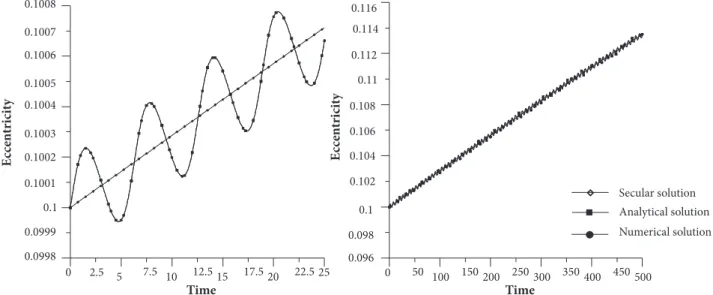
Figure 3. Comparison between secular, analytical and numerical time evolution of eccentricity for maneuver 1 with t
f – t0 = 25.0 and tf – t0 = 500.0.
Figure 4. Comparison between secular, analytical and numerical time evolution of inclination of orbital plane for maneuver 1 with t
f – t0 = 25.0 and tf – t0 = 500.0.
Secular solution Analytical solution Numerical solution
0 2.5 5 7.5 10 12.515 17.520 22.525
Time E cc en tr ic it y E cc en tr ic it y 0.0998 0.1 0.1002 0.1004 0.1006 0.1008 0.0999 0.1001 0.1003 0.1005 0.1007
0 50 100 150200 250300 350400 450500
Time 0.096 0.1 0.104 0.108 0.112 0.116 0.098 0.102 0.106 0.11 0.114 Secular solution Analytical solution Numerical solution
0 2.5 5 7.5 10 12.5 15 17.5 20 22.5 25
Time I nclina ti o n I nclina ti o n 10 10.02 10.04 10.06 10.08 10.1 10.01 10.03 10.05 10.07 10.09
0 50 100150 200250 300350 400 450 500
10 10.5 11 11.5 12 12.5 10.25 10.75 11.25 11.75 12.25
Table 1. Set of initial conditions and transfer duration.
State and adjoint variables Maneuver 1 Maneuver 2
a0 1.00 1.00
e0 0.10 0.10
I0 (degrees) 10.0 10.0
pa0 4.90002 × 10⁻⁵ 6.07832 × 10⁻⁴
pe0 1.15518 × 10⁻⁵ 1.92206 × 10⁻⁴
pI0 1.28967 × 10⁻⁴ 3.99208 × 10⁻⁴
J. Aerosp. Technol. Manag., São José dos Campos, v10, e1918, 2018 Table 2. Final state variables.
Maneuver
State variables Analytical theory Numerical solution
Secular solution Complete solution Runge-Kutta-Fehlberg 4-5
t
f – t0 25 500 25 500 25 500
1
af 1.00491 1.10294 1.00489 1.10294 1.00489 1.10294
ef 0.10071 0.11348 0.10066 0.11349 0.10066 0.11349
If (degrees) 10.09730 12.05344 10.09684 12.05351 10.09684 12.05351
Jf 2.3338 × 10⁻⁷ 4.6678 × 10⁻⁶ 2.3205 × 10⁻⁷ 4.6678 × 10⁻⁶ 2.3200 × 10⁻⁷ 4.6680 × 10⁻⁶
2
af 1.06354 5.06122 1.06199 4.91725 1.06199 4.92809
ef 0.11222 0.43929 0.10953 0.41415 0.10952 0.41691
If (degrees) 10.31167 32.02676 10.31524 32.52541 10.31515 32.26476
Jf 2.0662 × 10⁻⁵ 4.1324 × 10⁻⁴ 1.9995 × 10⁻⁵ 4.1229 × 10⁻⁴ 1.9986 × 10⁻⁵ 4.1111 × 10⁻⁴
Figure 5. Comparison between secular, analytical and numerical time evolution of semi-major axis for maneuver 2 with t
f – t0 = 25.0 and tf – t0 = 500.0.
Secular solution Analytical solution Numerical solution
0 2.5 5 7.5 10 12.5 15 17.5 20 22.5 25
Time Time
S
emi ma
jo
r axis
S
emi ma
jo
r axis
1 1.02 1.04 1.06 1.08
1.01 1.03 1.05 1.07
0 50 100 150 200 250 300 350 400 450 500 1
2 3 4 5 6
1.5 2.5 3.5 4.5 5.5
in degrees. It should be noted that similar results can be obtained for maneuver with modification of the ascending node, since this maneuver is equivalent to the one with modification of the inclination of the orbital plane, taking into account the conditions described earlier (see paragraph after Eqs. 2-7). For simplicity, the results refer to maneuvers with modification of the orbital plane.
used in the solution of the two-point boundary value problem of going from an initial orbit to a final orbit, as previously described. This last remark is relevant, since the numerical algorithm to compute optimal low-thrust trajectories based on the analytical solution requires a simple Newton-Raphson method to solve the two-point boundary value problem, as described above.
Figure 6. Comparison between secular, analytical and numerical time evolution of eccentricity for maneuver 2 with t
f – t0 = 25.0 and tf – t0 = 500.0.
Figure 7. Comparison between secular, analytical and numerical time evolution of inclination of orbital plane for maneuver 2 with t
f – t0 = 25.0 and tf – t0 = 500.0.
Secular solution Analytical solution Numerical solution
0 2.5 5 7.5 10 12.5 15 17.5 20 22.5 25 Time E cc en ti cit y E cc en ti cit y 0.096 0.1 0.104 0.108 0.112 0.116 0.098 0.102 0.106 0.11 0.114
0 50 100 150 200 250 300 350 400 450 500 Time 0 0.1 0.2 0.3 0.4 0.5 0.05 0.15 0.25 0.35 0.45 Secular solution Analytical solution Numerical solution 0 2.5 5 7.5 10 12.5 15 17.5 20 22.5 25
Time I nclina ti o n I nclina ti o n 10 10.1 10.2 10.3 10.4 10.05 10.15 10.25 10.35
0 50 100 150 200 250 300 350 400 450 500
Time 10 15 20 25 30 35 12.5 17.5 22.5 27.5 32.5 INDIRECT PROBLEM
J. Aerosp. Technol. Manag., São José dos Campos, v10, e1918, 2018 Of :(af , ef , θf ) at the prescribed final time tf is obtained considering the two versions of the analytical solution: the complete non-linear solution and the simplified linear solution for transfers between close orbits. This analysis allows us to discuss the applicability of the linear solution. Eight different maneuvers are considered, as described in Table 3. The initial orbit O0 is the same for all maneuvers and it is defined by the following set of orbital elements: a0 = 1.0 canonical unit, e0 = 1.0 and I0 = 1.0 degrees. The final value of the consumption variable J is taken as a comparison parameter for five transfer durations. Table 4 shows the results obtained through the two analytical solutions. JNon-linear is the consumption variable computed by Eq. 60, and JLinear is the consumption variable computed by Eq. 80. In both cases, variable J is expressed in canonical units. Figures 8-13 show
Maneuver tf – t0 JLinear JNon-linear Maneuver tf – t0 JLinear JNon-linear
1
5 1.2257 × 10-04 1.2243 × 10-04
5
5 5.1744 × 10-03 6.0723 × 10-03
10 5.7262 × 10-05 5.7226 × 10-05 10 2.2223 × 10-03 2.1756 × 10-03
15 3.9004 × 10-05 3.9128 × 10-05 15 1.7213 × 10-03 2.0148 × 10-03
20 2.8566 × 10-05 2.8568 × 10-05 20 1.1276 × 10-03 1.2010 × 10-03
25 2.3348 × 10-05 2.3352 × 10-05 25 1.0282 × 10-03 1.1878 × 10-03
2
5 8.4019 × 10-03 8.7410 × 10-03
6
5 5.2947 × 10-03 5.8923 × 10-03
10 3.2064 × 10-03 3.6288 × 10-03 10 2.0128 × 10-03 2.0770 × 10-03
15 2.7985 × 10-03 2.9243 × 10-03 15 1.7472 × 10-03 1.9542 × 10-03
20 1.7661 × 10-03 1.9309 × 10-03 20 1.0867 × 10-03 1.1831 × 10-03
25 1.6413 × 10-03 1.7601 × 10-03 25 1.0112 × 10-03 9.9530 × 10-04
3
5 8.3527 × 10-03 1.0240 × 10-02
7
5 4.8712 × 10-03 5.2944 × 10-03
10 5.3048 × 10-03 4.8075 × 10-03 10 2.1484 × 10-03 2.2786 × 10-03
15 2.7761 × 10-03 3.4134 × 10-03 15 1.6252 × 10-03 1.7622 × 10-03
20 2.4108 × 10-03 2.4108 × 10-03 20 1.1214 × 10-03 1.1969 × 10-03
25 1.6888 × 10-03 2.0480 × 10-03 25 9.6155 × 10-04 9.6277 × 10-04
4
5 4.7730 × 10-04 4.9924 × 10-04
8
5 5.3652 × 10-03 5.8071 × 10-03
10 1.8159 × 10-04 1.8234 × 10-04 10 2.2580 × 10-03 2.4075 × 10-03
15 1.1375 × 10-04 1.1402 × 10-04 15 1.7871 × 10-03 1.9357 × 10-03
20 9.3576 × 10-05 9.3779 × 10-05 20 1.1957 × 10-03 1.2827 × 10-03
25 7.6080 × 10-05 7.6363 × 10-05 25 1.0520 × 10-03 1.0449 × 10-03
Table 3. Set of terminal orbits.
Maneuvers
Terminal orbits
a
f (canonical units) ef If (degree)
1 1.05 0.105 11
2 1.50 0.45 12
3 2.00 0.25 15
4 1.10 0.15 11
5 1.60 0.25 11
6 1.50 0.30 12
7 1.50 0.20 15
8 1.50 0.25 15
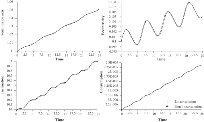
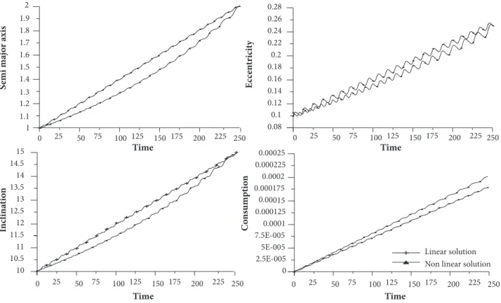
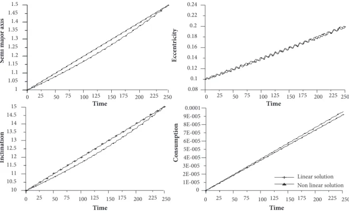
the time evolution of the semi-major axis, the eccentricity, the inclination of the orbital plane and the consumption variable for maneuvers 1, 3 and 7. Two transfer durations are considered: tf – t0 = 25.0 and tf – t0 = 250.0 time units. All variables are expressed in canonical units, except the inclination of the orbital plane, given in degrees. It should be noted that there exists a good agreement between the two analytical solutions, linear and non-linear, for maneuver 1, which corresponds to a transfer between close orbits. On the other hand, for maneuver 3, which corresponds to a transfer with moderate amplitude, the results given by the linear solution are not good. Similar conclusion applies to maneuver 7, although the behavior for larger duration transfer is fair.
Now, consider the problem of solving the two-point boundary value problem for long-time transfers using the secular solution and the complete analytical solution, which includes the short periodic terms. In order to compare these solutions, maneuver 3 described in Table 3 is considered, with two transfer durations, tf – t0 = 125.0 and 500.0 time units. Table 5 shows the initial value of the adjoint variables obtained by using the secular solution and by using the complete solution. Note that there exist small differences between these initial values. As previously described, a small adjust of the initial value of the adjoint variables is made by a Newton-Raphson algorithm when the short periodic terms are included. Note that this adjust become smaller for a very large transfer duration. Moreover, Figs. 14-16 show that the secular solution of the TPBVP does not represent a mean solution of the complete solution of the same TPBVP.
Figure 17 represents the optimal trajectory for maneuver 3 with time of flight equal to 125.0 time units. Note that the motion of the vehicle resembles a spiral, departing from the initial orbit and arriving at the terminal orbit after twelve revolutions around the central body. If the maneuver represents a transfer between two orbits around the Earth with the semi-major axis of the initial orbit, a0 = 1.0 distance unit, corresponding to 8000 km, then the maneuver lasts 39.35 hours and the magnitude of the average acceleration is equal to 1.59 cm/s2. For such maneuver, the ratio between the average acceleration and the gravity acceleration on
the ground is approximately 1.6 × 10⁻³, a typical value for low-thrust propulsion system. Similar conclusions are obtained for the
other maneuvers discussed in this section.
Time Time Time 0.106 0.108 0.107 0.103 0.105 0.104 0.1 0.102 0.101 0.098 0.099 0 2.5 5 7.5 10 12.5 15 17.5 20 22.5 25
0 2.5 5 7.5 10 12.5 15 17.5 20 22.5 25 0 2.5 5 7.5 10 12.5 15 17.5 20 22.5 25
0 2.5 5 7.5 10 12.5 15 17.5 20 22.5 25 Time C on su m p ti on E cc en tr ic it y Inclina ti o n S emi ma jo r axis Linear solution
Non linear solution 1 1.02 1.04 1.06 1.01 1.03 1.05 10 10.2 10.4 10.6 10.8 11 10.1 10.3 10.5 10.7 10.9 0 5E-006 1E-005 1.5E-005 2E-005 2.5E-005 2.5E-006 7.5E-006 1.25E-005 1.75E-005 2.25E-005
Figure 8. Time evolution of state variables for maneuver 1 with tf – t
J. Aerosp. Technol. Manag., São José dos Campos, v10, e1918, 2018
Time Time
0 25 50 75 100 125 150 175 200 225 250
Time 0.104 0.106 0.105 0.101 0.103 0.102 0.098 0.1 0.099 0 25 50 75 100 125 150 175 200 225 250
0 50 100 150 200 250
25 75 125 175 225
0 25 50 75 100 125 150 175 200 225 250 Time C on su m p ti on E cc en tr ic it y Inclina ti o n S emi ma jo r axis Linear solution
Non linear solution 1 1.02 1.04 1.06 1.01 1.03 1.05 10 10.2 10.4 10.6 10.8 11 10.1 10.3 10.5 10.7 10.9 0 5E-007 1E-006 1.5E-006 2E-006 2.5E-006 2.5E-007 7.5E-007 1.25E-006 1.75E-006 2.25E-006 Time Time
0 2.5 5 7.5 10 12.5 15 17.5 20 22.5 25
Time 10 11 12 13 14 15 10.5 11.5 12.5 13.5 14.5
0 2.5 5 7.5 10 12.5 15 17.5 20 22.5 25 0 2.5 5 7.5 10 12.5 15 17.5 20 22.525
0 2.5 5 7.5 10 12.5 15 17.5 20 22.5 25
Time C on su m p ti on E cc en tr ic it y Inclina ti o n S emi ma jo r axis Linear solution
Non linear solution 0 0.0005 0.001 0.0015 0.002 0.0025 0.00025 0.00075 0.00125 0.00175 0.00225 0.08 0.12 0.16 0.2 0.24 0.28 0.32 0.1 0.14 0.18 0.22 0.26 0.3 1 1.2 1.4 1.6 1.8 2 1.1 1.3 1.5 1.7 1.9
Figure 9. Time evolution of state variables for maneuver 1 with t
f – t0 = 250.0.
Figure 10. Time evolution of state variables for maneuver 3 with tf – t
Time Time
0 25 50 75 100 125 150 175 200 225 250
Time 10 11 12 13 14 15 10.5 11.5 12.5 13.5 14.5 0 25 50 75 100 125 150 175 200 225 250
0 50 100 150 200 250
25 75 125 175 225
0 25 50 75 100 125 150 175 200 225 250 Time C on su m p ti on E cc en tr ic it y Inclina ti o n S emi ma jo r axis Linear solution
Non linear solution 1 1.2 1.3 1.1 1.4 1.6 1.8 2 1.5 1.7 1.9 0.08 0.12 0.16 0.2 0.24 0.28 0.1 0.14 0.18 0.22 0.26 0 5E-005 0.0001 0.00015 0.0002 0.00025 2.5E-005 7.5E-005 0.000125 0.000175 0.000225
0 2.5 5 7.5 10 12.5 15 17.5 20 22.5 25
Time 1 1.1 1.2 1.3 1.4 1.5 1.05 1.15 1.25 1.35 1.45
0 5 10 15 20 25
2.5 7.5 12.5 17.5 22.5
Time 0.08 0.12 0.16 0.2 0.24 0.1 0.14 0.18 0.22
0 2.5 5 7.5 10 12.5 15 17.5 20 22.5 25
Time 10 11 12 13 14 15 10.5 11.5 12.5 13.5 14.5
0 2.5 5 7.5 10 12.5 15 17.5 20 22.5 25
Time C on su m p ti on E cc en tr ic it y Inclina ti o n S emi ma jo r axis 0 0.0002 0.0004 0.0006 0.0008 0.001 0.0001 0.0003 0.0005 0.0007 0.0009 Linear solution
Non linear solution Figure 11. Time evolution of state variables for maneuver 3 with t
f – t0 = 250.0.
Figure 12. Time evolution of state variables for maneuver 7 with tf – t
J. Aerosp. Technol. Manag., São José dos Campos, v10, e1918, 2018 Time 1 1.1 1.2 1.3 1.4 1.5 1.05 1.15 1.25 1.35 1.45 Time 0.08 0.12 0.16 0.2 0.24 0.1 0.14 0.18 0.22
0 25 50 75 100 125 150 175 200 225 250 Time 10 11 12 13 14 15 10.5 11.5 12.5 13.5 14.5 0 25 50 75 100 125 150 175 200 225 250
0 50 100 150 200 250
25 75 125 175 225
0 25 50 75 100 125 150 175 200 225 250 Time C on su m p ti on E cc en tr ic it y Inclina ti o n S emi ma jo r axis 0 2E-005 4E-005 6E-005 8E-005 0.0001 1E-005 3E-005 5E-005 7E-005 9E-005 Linear solution Non linear solution
Figure 13. Time evolution of state variables for maneuver 7 with tf – t
0 = 250.0.
Table 5. Initial value of the adjoint variables.
Maneuver Secular solution Complete solution
3
T
p
a0p
e0p
I0p
a0p
e0p
I0125 0.001203 0.000370 0.000837 0.001215 0.000384 0.000801
500 0.000300 0.000092 0.000209 0.000301 0.000093 0.000207
Figure 14. Secular solution and complete analytical solution of the TPBVP for maneuver 3 for both transfer durations – evolution of semi-major axis.
Time S emi-ma jo r axis S emi-ma jo r axis Secular solution Analytical solution Time
0 20 40 60 80 100 120 140 160 1 1.2 1.4 1.6 1.8 2 1.1 1.3 1.5 1.7 1.9
Figure 17. Optimal trajectory for maneuver 3 with t
f - to = 125.0.
Figure 15. Secular solution and complete analytical solution of the TPBVP for maneuver 3 for both transfer durations – evolution of eccentricity.
Figure 16. Secular solution and complete analytical solution of the TPBVP for maneuver 3 for both transfer durations – evolution of inclination of orbital plane.
X Axis Initial trajectory Optimal trajectory Final trajectory Y Axis Z Axis
0 20 40 60 80 100 120 140 160
Time 10 11 12 13 14 15 10.5 11.5 12.5 13.5 14.5 I nclina ti o n I nclina ti o n Secular solution Analytical solution
0 50 100 150 200 250 300 350 400 450 500
Time 10 11 12 13 14 15 10.5 11.5 12.5 13.5 14.5 Time E cc en tr ic it y E cc en tr ic it y Secular solution Analytical solution Time
0 20 40 60 80 100 120 140 160
0.08 0.12 0.16 0.2 0.24 0.28 0.1 0.14 0.18 0.22 0.26
0 50 100 150 200 250 300 350 400 450 500
J. Aerosp. Technol. Manag., São José dos Campos, v10, e1918, 2018
CONCLUSION
An approximated first-order analytical solution for optimal time-fixed low-thrust limited power transfers (no rendezvous) between elliptic coaxial non-coplanar orbits in an inverse-square force field is determined through canonical transformation theory. The existence of conjugate point for long duration transfers is investigated through Jacobi condition. For transfers between close orbits a simplified solution is straightforwardly obtained by linearizing the new Hamiltonian and the generating function obtained through Hori method. For the direct problem of generating extremals trajectories, the analytical solution is compared to the numerical solution obtained by integrating the canonical system of differential equations describing the extremal trajectories for some sets of initial conditions, and the accuracy of the analytical approach is established. For the indirect problem, an iterative algorithm based on the first-order analytical solution is described for solving the two-point boundary value problem of going from an initial orbit to a final orbit. A comparison between the linearized and nonlinear analytical solutions is made and it has been noticed that the linearized solution can provide good results for transfers between close orbits.
ACKNOWLEDGEMENTS
This research has been supported by CNPq under contract 304913/2013-8 and by FAPESP under contract 2012/21023-6.
AUTHOR’S CONTRIBUTIONS
Both authors contributed equally on this paper.
REFERENCES
Battin RH (1987) An introduction to the mathematics and methods of astrodynamics. New York: American Institute of Aeronautics and Astronautics, 796 p.
Bliss GA (1946) Lectures on the calculus of variations. Chicago: University of Chicago Press.
Bonnard B, Caillau JB, Dujol R (2006) Averaging and optimal control of elliptic Keplerian orbits with low propulsion. Systems & Control Letters 55(9):755-760. doi: 10.1016/j.sysconle.2006.03.004
Camino O, Alonso M, Blake R, Milligan D, Bruin JD, Ricken S (2005) SMART-1: Europe’s Lunar Mission Paving the Way for New Cost Effective Ground Operations (RCSGSO), Sixth International Symposium Reducing the Costs of Spacecraft Ground Systems and Operations (RCSGSO), European Space Agency ESA SP-601; Darmstadt, Germany.
da Silva Fernandes S (2003) Notes on Hori method for canonical systems. Celestial Mechanics and Dynamical Astronomy 85(1):67-78. doi: 10.1023/a:1021711221662
da Silva Fernandes S, das Chagas Carvalho F (2008) A first-order analytical theory for optimal low-thrust limited-power transfers between arbitrary elliptical coplanar orbits. Mathematical Problems in Engineering 2008. doi: 10.1155/2008/525930
da Silva Fernandes S, das Chagas Carvalho F, de Moraes RV (2015) Optimal low-thrust transfers between coplanar orbits with small eccentricities. Computational and Applied Mathematics 1-14. doi: 10.1007/s40314-015-0249-9
Edelbaum TN (1964) Optimum low-thrust rendezvous and station keeping. AIAA Journal 2(7):1196-1201. doi: 10.2514/3.2521
Edelbaum TN (1965) Optimum power-limited orbit transfer in strong gravity fields. AIAA Journal 3(5):921-925. doi: 10.2514/3.3016
Edelbaum TN (1966) An asymptotic solution for optimum power limited orbit transfer. AIAA Journal 4(8):1491-1494. doi: 10.2514/3.3725
Forsythe GE, Malcolm MA, Moler CB (1977) Computer methods for mathematical computations. Englewood Cliffs, New Jersey 07632. Prentice Hall, Inc., XI, 259 S. doi: 10.1002/zamm.19790590235
Geffroy S, Epenoy R (1997) Optimal low-thrust transfers with constraints-generalization of averaging techniques. Acta Astronautica 41(3):133-149. doi: 10.1016/s0094-5765(97)00208-7
Gobetz FW (1964) Optimal variable-thrust transfer of a power-limited rocket between neighboring circular orbits. AIAA Journal 2(2):339-343. doi: 10.2514/3.2281
Gobetz FW (1965) A linear theory of optimum low-thrust rendezvous trajectories. Journal of the Astronautical Sciences 12:69.
Haissig CM, Mease KD, Vinh NX (1993) Minimum-fuel, power-limited transfers between coplanar elliptical orbits. Acta Astronautica 29(1):1-15. doi: 10.1016/0094-5765(93)90064-4
Hori GI (1966) Theory of general perturbation with unspecified canonical variable. Publications of the Astronomical Society of Japan 18(4):287-296.
Huang W (2012) Solving coplanar power-limited orbit transfer problem by primer vector approximation method. International Journal of Aerospace Engineering. doi: 10.1155/2012/480320
Jamison BR, Coverstone V (2010) Analytical study of the primer vector and orbit transfer switching function. Journal of Guidance, Control, and Dynamics 33(1):235-245. doi: 10.2514/1.41126
Jiang F, Baoyin H, Li J (2012) Practical techniques for low-thrust trajectory optimization with homotopic approach. Journal of Guidance, Control, and Dynamics 35(1):245-258. doi: 10.2514/1.52476
Kiforenko BN (2005) Optimal low-thrust orbital transfers in a central gravity field. International Applied Mechanics 41(11):1211-1238. doi: 10.1007/s10778-006-0028-9
Lanczos C (1970) The variational principles of mechanics. 4th edition. Toronto: University of Toronto Press.
Lie S (1888) Theorie der transformationsgruppen I. Leipzig: Teubner.
Marec JP (1979) Optimal space trajectories. New York: Elsevier.
Marec JP, Vinh NX (1980) Étude generale des transferts optimaux a poussee faible et puissance limitee entre orbites elliptiques quelconques. ONERA Publication 1980-1982.
Marec JP, Vinh NX (1977) Optimal low-thrust, limited power transfers between arbitrary elliptical orbits. Acta Astronautica 4(5-6):511-540. doi: 10.1016/0094-5765(77)90106-0
Pines S (1964) Constants of the motion for optimum thrust trajectories in a central force field. AIAA Journal 2(11):2010-2014. doi: 10.2514/3.2717
Pontryagin LS, Boltyanskii VG, Gamkrelidze RV, Mishchenko EF (1962) The mathematical theory of optimal control processes. New York: John Wiley & Sons. 357 p.
Quarta AA, Mengali G (2013) Trajectory approximation for low-performance electric sail with constant thrust angle. Journal of Guidance, Control, and Dynamics 36(3):884-887. doi: 10.2514/1.59076
Racca GD (2003) New challengers to trajectory design by the use of electric propulsion and other new means wandering in the solar system. Celestial Mechanics and Dynamical Astronomy 85(1):1-24. doi: 10.1023/a:1021787311087
Racca GD, Marini A, Stagnaro L, van Dooren J, di Napoli L, Foing BH, Lumb R, Volp J, Brinkmann J, Grünagel R et al. (2002) SMART-1 mission description and developments status. Planetary and Space Science 50:1323-1336. doi:10.1016/S0032-0633(02)00123-X
Rayman MD, Varghese P, Lehman DH, Livesay LL (2000) Results from the Deep Space 1 technology validation mission. Acta Astronautica 47(2-9):475-487. doi: 10.1016/s0094-5765(00)00087-4
Stoer J, Bulirsch R (2002) Introduction to numerical analysis. 3rd edition. New York, USA: Springer.