Modelling approach to the assessment of biogenic fluxes at a selected Ross Sea site, Antarctica

(1)

OSD

6, 1477–1512, 2009

Modelling vertical biogenic fluxes in the

Ross Sea

M. Vichi et al.

Title Page

Abstract Introduction

Conclusions References

Tables Figures

◭ ◮

Back Close

Full Screen / Esc

Printer-friendly Version

Interactive Discussion

Ocean Sci. Discuss., 6, 1477–1512, 2009 www.ocean-sci-discuss.net/6/1477/2009/

Ocean Science Discussions

Papers published inOcean Science Discussionsare under open-access review for the journalOcean Science

Modelling approach to the assessment of

biogenic fluxes at a selected Ross Sea

site, Antarctica

M. Vichi1,2, A. Coluccelli2,*, M. Ravaioli3, F. Giglio3, L. Langone3, M. Azzaro4, F. Azzaro4, R. La Ferla4, G. Catalano5, and S. Cozzi5

1

Centro Euro-Mediterraneo per i Cambiamenti Climatici, Bologna, Italy

2

Istituto Nazionale di Geofisica e Vulcanologia, Bologna, Italy

3

CNR-ISMAR Sezione di Bologna, Via Gobetti 101, 40129 Bologna, Italy

4

CNR-IAMC Sezione di Messina, Spianata S. Ranieri 86, 82122 Messina, Italy

5

CNR-ISMAR Sezione di Trieste, V. le Gessi 2, 34123 Trieste, Italy

*

now at: Universit ´a Politecnica delle Marche, Ancona, Italy

Received: 28 May 2009 – Accepted: 29 June 2009 – Published: 8 July 2009

Correspondence to: M. Vichi ([email protected])

(2)

OSD

6, 1477–1512, 2009

Ross Sea

M. Vichi et al.

Title Page

Tables Figures

◭ ◮

Back Close

Full Screen / Esc

Abstract

Several biogeochemical data have been collected in the last 10 years of Italian ac-tivity in Antarctica (ABIOCLEAR, ROSSMIZE, BIOSESO-I/II). A comprehensive 1-D biogeochemical model was implemented as a tool to link observations with processes and to investigate the mechanisms that regulate the flux of biogenic material through

5

the water column. The model is ideally located at station B (175◦E–74◦S) and was set up to reproduce the seasonal cycle of phytoplankton and organic matter fluxes as forced by the dominant water column physics over the period 1990–2001. Austral spring-summer bloom conditions are assessed by comparing simulated nutrient draw-down, primary production rates, bacterial respiration and biomass with the available

10

observations. The simulated biogenic fluxes of carbon, nitrogen and silica have been compared with the fluxes derived from sediment traps data. The model reproduces the observed magnitude of the biogenic fluxes, especially those found in the bottom sed-iment trap, but the peaks are markedly delayed in time. Sensitivity expersed-iments have shown that the characterization of detritus, the choice of the sinking velocity and the

15

degradation rates are crucial for the timing and magnitude of the vertical fluxes. An increase of velocity leads to a shift towards observation but also to an overestimation of the deposition flux which can be counteracted by higher bacterial remineralization rates. Model results suggest that the timing of the observed fluxes depends first and foremost on the timing of surface production and on a combination of size-distribution

20

and quality of the autochtonous biogenic material. It is hypothesized that the bottom sediment trap collects material originated from the rapid sinking of freshly-produced particles and also from the previous year’s production period.

1 Introduction

More than 10 years of physical and biogeochemical measurements have been

col-25

(3)

Pro-OSD

6, 1477–1512, 2009

Ross Sea

M. Vichi et al.

Title Page

Tables Figures

◭ ◮

Back Close

Full Screen / Esc

getto Nazionale di Ricerca in Antartide). These data represent a valuable set of in-formation on the dynamical variability of polar ecosystems and can be profitably used to constrain biogeochemical models of the global ocean carbon cycle in the Southern Ocean. On the other hand, models can also be used to support the interpretation of observations, as tools to link data with processes and to investigate the complex

5

mechanisms that regulate the flux of biogenic material through the water column. We have a fragmented picture of the plankton seasonal cycle in the Ross Sea, mostly derived from composites of diverse biogeochemical data collected in di_fferent years (Smith et al., 1996, 2000; Lipizer et al., 2000; Smith and Asper, 2001; Azzaro et al., 2006). Little synoptic observations are available, and the longer seasonal time-series

10

on biogenic components are obtained from sediment trap measurements (Collier et al., 2000; Langone et al., 2000). Phytoplankton growth in the Ross Sea usually initiates in early spring, much earlier than in other regions of the Antarctic, likely because of favourable stratification conditions induced by ice melting (Smith and Asper, 2001). The patchy structure of this process is therefore responsible for the large spatial

vari-15

ability of growth conditions. After the onset of stratification, the spring-summer period is characterized by spatially-extended blooms dominated by diatoms in the north-eastern open water part and by the colonial prymnesiophytePhaeocystis Antarcticain seasonal ice zones and coastal waters (DiTullio et al., 2000; DiTullio and Smith, 1996).

The vertical fluxes of biogenic material are characterized by the occurrence of rapid

20

sinking events (DiTullio et al., 2000; Asper and Smith, 2003; Langone et al., 2003), time-extended small deposition rates that lag the production peak of some months (Gardner et al., 2000; Collier et al., 2000) or by a combination of both phenomena (Langone et al., 2000). It is thus difficult to assess their role in influencing CO2fluxes with the atmosphere and the export rates of organic carbon to the deep ocean.

Or-25

(4)

OSD

6, 1477–1512, 2009

Ross Sea

M. Vichi et al.

Title Page

Tables Figures

◭ ◮

Back Close

Full Screen / Esc

et al., 2000; Langone et al., 2000). This suggests that processes other than surface ex-port modify the characteristics of the sinking material, the more likely being horizontal advective transport and aggregation mechanisms.

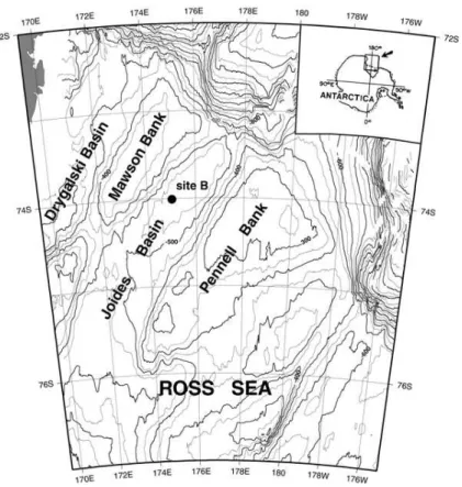
To partly bridge the gaps among these contrasting information, we have implemented a coupled physical-biogeochemical model at station B (175◦_E–74◦_{S, central Joides}

5

basin, Fig. 1) of the PNRA Italian programme, with the aim to reproduce the vertical fluxes of autochtonous organic matter as forced by the dominant water column physics. The ultimate scope of the simulation is thus not to fit the sparse observations, but rather to provide the dynamical framework for hypotheses testing, assessing the model pre-diction against the available standing stock and rate measurements collected during

10

the Italian and international joint projects (ABIOCLEAR, ROSSMIZE and BIOSESO-I/II). Particularly, this work will focus on the assessment of the vertical fluxes of organic particles and the comparison with data collected in sediment traps. Station B was cho-sen for several reasons: the more simple physical conditions due to the abcho-sence of polynia, a diatom-dominated bloom instead of Phaeocystys (which reduces the

com-15

plexity of the phytoplankton parameterization) and also because many open questions still remain on the vertical dynamics inferred from sediment traps with respect to other more typical mooring sites (station A, 76.8◦S 169◦E, Langone et al., 2003)

The next section gives some details on the model features and the interannual forcing functions used to drive the one-dimensional simulation. Section 3 presents model

20

results organized following these major guidelines:

– quantification of the organic matter production in the euphotic layer and compari-son with available observations;

– quantification of heterotrophic consumption processes in the mesopelagic layer;

– estimation of model-derived sinking rates at given depths within the aphotic zone;

25

(5)

OSD

6, 1477–1512, 2009

Ross Sea

M. Vichi et al.

Title Page

Tables Figures

◭ ◮

Back Close

Full Screen / Esc

Section 3.6 gives an overview of the model sensitivity to the key parameters affecting the vertical fluxes such as sinking velocity and bacterial remineralization rates. The outcomes of the experiments are discussed in Sect. 4 and, finally, Sect. 5 offers some conclusion remarks.

2 The simulation tool

5

The modelling framework is derived from the system set up by Vichi et al. (2004)

to study the open Baltic biogeochemistry. The physical model is a vertical

one-dimensional version of the Princeton Ocean Model (Blumberg and Mellor, 1987, POM), where the dynamical core is the turbulence closure scheme proposed by Mellor and Yamada (1982). The total depth of the water column is 588 m and the discrete vertical

10

grid is composed of 30 levels, 5 in the first 20 m with a depth increasing from 1 to 10 m, and the reminder with a constant depth of 22 m.

The Biogeochemical Flux Model (BFM, http://bfm.cmcc.it) was developed as a gen-eralized modelling tool to be coupled to several kind of hydrodynamic models. This model was also applied to the world ocean ecosystem with a global configuration

15

named PELAGOS (PELAgic biogeochemistry for Global Ocean Simulations Vichi et al., 2007a,b). A formal background theory of the model applied to the global ocean is found in Vichi et al. (2007a). The model version used in this application is the standard BFM configuration with the addition of the iron dynamics used in PELAGOS and the further implementation of two forms of sinking organic detritus (cf. Sect. 2.2).

20

The biogeochemistry model is essentially a biomass-based set of differential equa-tions that allows the simulation of lower trophic levels and major inorganic and organic components of the marine ecosystem. The model is based on the definition of Chem-ical Functional Families (CFF, Vichi et al., 2007a), which are theoretChem-ical constructs representing biogeochemical components in the Eulerian continuum and are further

25

(6)

OSD

6, 1477–1512, 2009

Ross Sea

M. Vichi et al.

Title Page

Tables Figures

◭ ◮

Back Close

Full Screen / Esc

organisms. LFGs are grouping of organisms according to their functional behavior in the ecosystem and not to phylogenetic considerations. Both CFFs and LFGs repre-sent the concentrations of measurable properties of marine biogeochemistry such as the carbon content in marine diatoms or the nitrogen contained in dissolved organic matter (Fig. 2). All the model state variables are expressed in terms of time-varying

5

basic components (both elements as C, N, P, Si, O, Fe or biochemical molecules as chl), whose relationships regulate the functioning of a specific LFG (as for instance the chl:C ratio in phytoplankton) or the actual availability (as the nutrient:C ratios in particulate detritus).

As depicted in Fig. 2, the model resolves 4 different LFGs for phytoplankton

(di-10

atoms, autotrophic nanoflagellates, picophytoplankton and large phytoplankton), 4 for zooplankton (carnivorous and omnivorous mesozooplankton, microzooplankton and heterotrophic nanoflagellates), 1 LFG for bacteria, 8 inorganic CFFs for nutrients and gases (phosphate, nitrate, ammonium, silicate, dissolved iron, reduction equivalents, oxygen, carbon dioxide) and 11 organic non-living CFFs for dissolved and particulate

15

detritus. With this kind of approach, all the nutrient:carbon ratios in chemical organic and living functional groups, as well as chl:C ratios in phytoplankton, are allowed to vary within their given ranges and each component has a distinct biological and physi-cal time rate of change. This kind of parameterization mimics the acclimation of organ-isms to the prevailing nutrients and light conditions, and allow the recycling of organic

20

matter to be functionally determined by the actual nutrient content.

2.1 Forcing functions and initial conditions

The model is forced with daily surface fluxes from the ERA40 data set over the period 1990–2001 (Uppala et al., 2005) in a 1◦

×1◦degrees region around station B. Daily sea

surface temperature (SST) data from the Reynolds data set (Reynolds, 1988) are also

25

(7)

OSD

6, 1477–1512, 2009

Ross Sea

M. Vichi et al.

Title Page

Tables Figures

◭ ◮

Back Close

Full Screen / Esc

the computed SST is below the freezing point, while the relaxation term is continuously given to allow the surface to shift from packed-ice to ice-free conditions as typical of this marginal ice zone. During the ice-free conditions the surface restoration term is negligible since the model responds correctly to the surface fluxes.

The model is initialized on 1 June 1990 with average winter temperature, salinity and

5

macronutrient profiles of the whole Ross Sea from the World Ocean Atlas (Conkright et al., 2002). Initial iron concentration is set to 0.25µmol m−3 as the average value measured by Sosik and Olson (2002) in the Ross Sea. Biogeochemical LFGs and CFFs are initialized with homogeneous low values mimicking the quiescent winter pe-riod. The model is robust to the choice of winter initial conditions for biogeochemical

10

variables in the sense that the di_fference in the solution trajectories of perturbed exper-iments (±20%) is limited to less than 5% after one year of simulation.

Nitrate, silicate and phosphate are dynamically relaxed to the background winter profiles with a 3 month time scale when the water column is under packed-ice condi-tions, parameterizing the replenishment of nutrients caused by non-resolved and

three-15

dimensional advection processes under sea ice.

2.2 Model adaptation

Organic particle dynamics is complex and as a first approximation linked to the con-stituents and dimensions of particles. The standard BFM configuration assumes that organic detritus can be described by one single class of medium-degradable organic

20

matter with a sinking speed of 1.5 m d−1

. This is a rough approximation because there is no distinction between denser, fast-sinking detrital material such as faecal pellets and other particulate excretion from smaller heterotrophs, lysis or sloppy feeding prod-ucts. To di_fferentiate between these groups an additional variable was introduced in the model representing the detritus produced by mesozooplankton (including biogenic

25

(8)

OSD

6, 1477–1512, 2009

Ross Sea

M. Vichi et al.

Title Page

Tables Figures

◭ ◮

Back Close

Full Screen / Esc

in the Ross Sea have in fact reported sinking speeds of organic aggregates of more than 250 m d−1(Asper and Smith, 2003). Sensitivity experiments have been carried out and presented in Sect. 3.6 to analyze the impact of different choices of the organic detritus parameterization on the results.

3 Simulation results

5

3.1 Water column physics

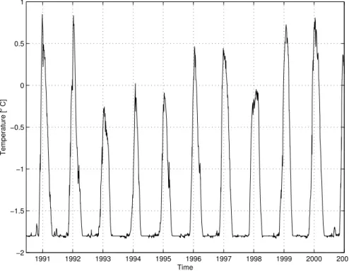
Figure 3 shows the time-series of the simulated SST, which is mostly controlled by the Reynolds data due to the imposed relaxation constraint. There is a clear interannual variability in the data which is also visible in the atmospheric forcing functions. The maxima in 1992 and 1997 are likely to be related to the large scale variability induced

10

by El Ni ˜no, for which correlations have been reported with sea-ice retreat in the Ross Sea (Ledley and Huang, 1997; Kwok and Comiso, 2002).

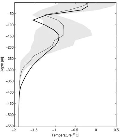
The long-term vertical structure computed by the model is comparable with the av-erage of the data collected during the deployment and monitoring of the mooring in the 1994–1998 summer campaigns (Fig. 4, Russo et al., 1997). The peculiar dicothermal

15

layer is rather well reproduced by the model. This cold water structure, constrained be-tween the surface warm waters above and the warmer but saltier waters below, is found in the surface layers of high latitude oceans generally between 50 and 150 m depth. Despite a slight discrepancy of 1 model level (22 m) in the location of the minimum, the vertical structure is in good agreement with the available observations, especially

20

in the simulation of the surface mixed layer depth.

3.2 Water column biogeochemistry

(9)

OSD

6, 1477–1512, 2009

Ross Sea

M. Vichi et al.

Title Page

Tables Figures

◭ ◮

Back Close

Full Screen / Esc

(Catalano et al., unpublished data). Data were collected in December 1994 before the starting of the bloom and during “lower” nutrient concentrations in January 1995 and 1996. Due to the low time resolution of data, it is not possible to infer a clear signal of the exact timing of the bloom. If we assume an ergodic hypothesis in the data distribution, we may say that the model broadly capture the range of the nutrient

5

drawdown. The most remarkable feature is the underestimation of the silicate uptake, which is low even if the simulated bloom is composed of about 60% diatoms and 40% nanoflagellates (not shown) and primary production is comparable with observations as described below. These results are obtained by taking into account an increased Si:C reference ratio of 3 times the standard BFM value due to the effects of Fe limitation

10

(Takeda, 1998; Lancelot et al., 2000), but still the model is not capable of reproducing the observed decrease in silicate concentration.

Autotrophic biomass (as chlorophyll concentration) and gross primary production (GPP) in the euphotic zone over the simulation period are shown in Fig. 6. Station B has a much lower biomass and production rates with respect to the stations in the

poly-15

nia open waters (Smith et al., 1996, 2000), although the marginal ice zone can reach substantially high production rates and concentrations during the Austral spring (Sag-giomo et al., 1998). The model simulates a bulk biomass and GPP rates which are comparable with the available observations (Saggiomo et al., 1998, 2002; Vaillancourt et al., 2003). GPP is highly correlated with SST in the model (r₌0.91,p<0.01) and the

20

periods with lower temperatures correspond to the minima of gross production. The chl content is instead less sensitive to temperature values but still significantly corre-lated (r₌0.68, p<0.01). The production peaks are earlier by about one month with respect to the biomass maxima as also observed in the polinya region (Smith et al., 2000). However, in contrast with the latter observations, the model indicates that the

25

(10)

OSD

6, 1477–1512, 2009

Ross Sea

M. Vichi et al.

Title Page

Tables Figures

◭ ◮

Back Close

Full Screen / Esc

Vaillancourt et al. (2003) reported some data on the light regime at station B (sta-tion “Sei” of the US-JGOFS programme) during the Austral summer of 1997. The euphotic zone depth was around 40 m and the light diffuse attenuation coefficient was 0.122 m−1. Simulated Chl concentration during this period is lower, and also the chl-specific primary production is about half the reported value of 11 mg C (mg chl)−1

d−1 .

5

The modeled euphotic zone depth is therefore slightly higher than observed. Further-more, this diffuse attenuation coefficient is only obtained in the simulation by assuming a background attenuation of 0.08 m−1_{(about twice the optical attenuation of pure}

sea-water) and a spectrally-integrated chl-specific light absorption of 0.03 (mg chl)−1m2. The reported values in the polynia region dominated by Phaeocystis Antarctica are

10

around 0.01 (mg chl)−1_m2 _{at the 676 nm red peak (Vaillancourt et al., 2003), but we}

may assume that a diatom-dominated population can have a larger value due to pig-ment packaging.

3.3 Phytoplankton light acclimation and growth rates

Several authors have suggested that phytoplankton assemblage in the Ross Sea is

15

adapted to low irradiance and therefore it should not be considered light-limited (Sag-giomo et al., 2002; Smith et al., 1996). It is thus important to verify that the model is capable of reproducing these conditions and particularly the low specific growth rates typical of this region (Smith et al., 1999). Figure 7a shows the simulated seasonal evolution in 1996–1998 of the realized chl:C ratio in surface diatoms, superimposed

20

to the optimal value that is used in the model to drive chl synthesis according to the Geider et al. (1996) parameterization. Low chl:C ratios are characteristic of the Ross Sea (Smith et al., 1996). In stations dominated by diatoms, the chl:C ratio was as low as 0.005 (DiTullio and Smith, 1996), which is a value also predicted by the model as the minimum allowed. It is interesting to note that the realized ratio varies less than

25

the potential value because of the water column mixing that homogenizes population adapted to different depths and light conditions.

(11)

com-OSD

6, 1477–1512, 2009

Ross Sea

M. Vichi et al.

Title Page

Tables Figures

◭ ◮

Back Close

Full Screen / Esc

puted with two different methods: i) estimated from the algebraic sum of the realized specific physiological rates of gross production, rest and activity respiration and activity excretion (cf. Fig. 2); ii) computed from the surface carbon biomass stored every day of simulation and according to the formula used in field estimates (Smith et al., 1999, 2000),

5

µ₌ 1

∆tln

_C

+ ∆C C

whereC is the biomass concentration and ∆C the biomass change in the sampling

interval∆t₌1 d. The estimated growth rates of diatoms with the latter method are ex-tremely low during the summer season, generally around 0.1 d−1 _{(Smith et al., 1999,}

2000). The model agrees well with these estimates, implying that the net carbon

pro-10

duction rates are reasonably simulated. However, these values are achieved only by applying a 0.5 coefficient to the non dimensional temperature regulating factor of phy-toplankton growth based on the Q10 function (Vichi et al., 2007a). Indeed, Smith et al. (1999) suggested that the maximum growth rates predicted by temperature-dependent exponential models could overestimate growth at temperature lower than 2◦C.

Gold-15

man and Carpenter (1974) values are in fact about half the ones parameterized with the Eppley curve. Model results also suggest that the choice of the method can lead to different values. The thick line in fact represents the growth induced by local light and nutrient conditions, as the one obtained from controlled on-deck incubations. It is also visible a decrease during the maximum productive periods due to self-shading effects.

20

The thin line is instead the realized change of mass due to a combination of physiolog-ical processes, vertphysiolog-ical mixing and grazing rates. This is more similar to what can be measured in-situ, and is less representative of the physiological state of phytoplankton.

3.4 Microbial respiration

Scarce information are available on the oxidation of organic matter in the mesopelagic

25

(12)

OSD

6, 1477–1512, 2009

Ross Sea

M. Vichi et al.

Title Page

Tables Figures

◭ ◮

Back Close

Full Screen / Esc

of microbial respiration in the aphotic zone, pointing out that about 63% of the organic carbon remineralized by respiration is derived from the detrital pool. Indeed, the model predict a very low concentration of DOC due to the excess of macronutrient availability, which reduces the release of polysaccharides from nutrient-limited autotrophic cells.

We have used the estimates of Azzaro et al. (2006) to assess the capability of

5

the model to reproduce the remineralization of organic matter in the mesopelagic layer. Figure 8 shows the simulated vertical distribution of microbial biomass and respiration rate during the period of the 2001 BIOSESO II campaign. The depth-integrated value of microbial biomass at site B in the mesopelagic layer (100–600 m), estimated from the measured ATP, varied from 480 to 840 mg C m−2, and the

depth-10

integrated respiration-derived carbon flux, calculated from direct ETS measurements, was 17.3 mg C m−2d−1. Both in the pre-bloom and bloom conditions (mid January and late February, respectively), the model shows a surface maximum of microbial respi-ration, with small subsurface maxima at 500 m. Microbial biomass shows the same pattern in January, with a relative maximum in the deeper part. In February, the larger

15

amount of freshly produced particles allows microorganisms to homogeneously dis-tribute over the whole water column, but still showing the maximum at 500 m. Microbial respiration eventually increases during late summer-autumn, following the bulk of or-ganic matter produced in the euphotic zone that reaches this depth in April–May (cf. sections below). Integrated values agree with the available observations, implying that

20

the bulk of the remineralization process is rather well captured by the model.

3.5 Simulated sediment trap fluxes

Fluxes at the depths of the real sediment trap locations were computed as the prod-uct of the prognostic detritus concentrations at the selected depths with the respective sinking velocity. Figure 9 shows the comparison of model results with the fluxes

esti-25

(13)

OSD

6, 1477–1512, 2009

Ross Sea

M. Vichi et al.

Title Page

Tables Figures

◭ ◮

Back Close

Full Screen / Esc

with the surface peaks in the modeled biomass, as indicated by the triangles in the up-per axes of each subplot. This implies that the occurrence of the peak in the simulated trap is linked to the timing of the bloom in the model, which is in turn linearly correlated with the SST.

On the other hand, the amplitude of the simulated C flux is in good agreement with

5

the observations, and also the increase between 1995 and 1996, which is explained by the model as a response to the changes in SST and surface primary production. The fluxes of organic N closely follow the time distribution both in the data and in the model, but are overestimated by a factor 2–3. BSi is instead underestimated with respect to the trap data, which is likely to be related to the low consumption of dissolved silicate

10

in the surface layers (Fig. 5).

The simulated deposition flux can be separated in the components due to the fast-sinking detritus produced by mesozooplankton and to the slow-fast-sinking detritus for the surface and bottom traps (Fig. 10, for the C component only). In contrast with the observations (Langone et al., 2000), the peak in the top trap (Fig. 10a) is higher than

15

the bottom trap during the productive phase and is mostly composed of large fast-sinking particles. The maximum of slow detritus is simulated in middle winter, with a lag of about 3 months with respect to the surface production peak as also found in other sediment trap data (Collier et al., 2000). The bottom trap (Fig. 10b) is instead characterized by a summer peak mostly composed of slow detritus produced in the

20

year before. This is followed by the peak of freshly-produced organic matter that sinks down with a velocity of 100 m d−1and reaches the bottom trap almost at the same time of the trap above. It is interesting to note that there are periods such as late-spring and early-summer in which the bottom trap simulated flux is larger than the one above as also found in the observations (Langone et al., 2000).

25

3.6 Sensitivity analysis

(14)

degrada-OSD

6, 1477–1512, 2009

Ross Sea

M. Vichi et al.

Title Page

Tables Figures

◭ ◮

Back Close

Full Screen / Esc

tion rates. Table 1 reports the experiments that have been performed and the effects on the simulated vertical carbon fluxes at the sediment traps are depicted in Fig. 11. Experiment D0 is the standard BFM setup with one single type of detritusR(6)(Fig. 2); experiment D5 is the reference simulation run that has been previously described.

The difference between D0 and D1 shows the effect of the addition of another detrital

5

component, R(5). With one slow-sinking detritus, the flux at the top trap is composed of one single peak that lags by 4 months the maximum of surface biomass and by 5 months the maximum of production. In D1, the addition of a relatively fast-sinking (10 m d−1_{) component produced by the diatom grazers shifts the surface peak towards}

the bloom period and reduces the winter maximum. The same also occurs to a lesser

10

extent in the bottom trap. The choice of the degradation rate ofR(5)detritus determines the amplitude of the summer peak. In run D2 the rate is decreased of 1 order of magnitude, while in D3 is set to 0.5 d−1, equivalent to the availability of freshly-produced DOM. It is important to remember that these coefficients represent the availability of substrate to bacteria. Part of the substrate available to bacteria is converted to CO₂

15

and biomass in the model, but a fraction of it is also moved to the slow-sinking and less degradable compartment simulating a decrease of the organic matter quality. When the degradation rate is slow as in D2, moreR(5)reaches both traps; when, conversely, the rate is higher as in D3 and the sinking rate is still 10 m d−1_{, almost no fast-sinking}

detritus is found.

20

Setting the sinking rate to 100 m d−1(run D4 and D5) shifts the deposition maxima towards the timing of the surface bloom but also lead to an overestimation of the de-position rates at both traps with respect to the observations. Only by assuming a large availability ofR(5)as in D5, the reference simulation, it is possible to obtain simulated fluxes which are comparable with the data. Noteworthily, and despite the large

overes-25

(15)

OSD

6, 1477–1512, 2009

Ross Sea

M. Vichi et al.

Title Page

Tables Figures

◭ ◮

Back Close

Full Screen / Esc

4 Discussion

The material collected in sediment traps is the result of a dynamical balance between the net export rate due to euphotic production, and the degradation and sinking rates, which are mostly determined by the size and quality of the particles. All these pro-cesses occur simultaneously in the upper ocean, and thus the estimation of vertical

5

fluxes by means of surface sediment traps is affected by several biases (Buesseler, 1991, 1998; Smith and Dunbar, 1998). The use of numerical models is a possible methodology to support the assessment of the organic matter fate in the deep ocean, particularly in key regions like the Southern Ocean where the collection of long term time-series is limited. Within the limits of the one-dimensional assumption, the

pro-10

duction of organic matter in the upper ocean was simulated as a function of physical conditions, light and nutrient availability, and the prognostic vertical flux of organic ma-terial at selected depths was used to compare with deep-ocean sediment traps. Com-prehensive biogeochemical models like the BFM can provide some of the dynamical linkages between observations derived from multidisciplinary campaigns. However,

15

biogeochemical models need to be applied with due attention, because of the many assumptions in the parameterization of physiological and ecological processes (Vichi et al., 2007a).

The BFM has many parameters which can be adjusted to reproduce the observed biogeochemical system behaviour. Data constraints in the Ross Sea region are limited

20

and therefore a complete model tuning is not feasible. Since the model was mostly developed for temperate regions, we have performed a set of classical sensitivity anal-ysis to identify the parameters which affect the biogeochemical processes under high latitude environmental conditions. The key parameters affecting the succession of phy-toplankton groups are the basal respiration rates which determine the survival standing

25

(16)

labo-OSD

6, 1477–1512, 2009

Ross Sea

M. Vichi et al.

Title Page

Tables Figures

◭ ◮

Back Close

Full Screen / Esc

ratory experiments of light deprivation when phytoplankton is brought back to sufficient irradiance levels after a dark period of several months (Peters and Thomas, 1996). The choice of the same respiration rate for diatoms and flagellates was necessary to obtain a dominance of diatoms but also a sufficient abundance of nanoflagellates, as observed in the station B area (Saggiomo et al., 2002).

5

Other important parameters are the availability coefficients of phytoplankton to graz-ers. Both grazing and iron are factors limiting the diatom bloom in the model. If iron limitation is deactivated in the model, the bloom is much larger and the time duration is totally controlled by grazing. The sensitivity of the model to grazing coefficients is rather high, particularly because the over-wintering biomass is small and an

exces-10

sive grazing pressure can completely deplete one of the phytoplankton group. This is for example the case of the simulated eukaryotic picophytoplankton, which is over-grazed by heterotrophic nanoflagellates living on bacteria. Nevertheless, it is difficult to assess the ecological relevance of this component (Vanucci and Bruni, 1998) and therefore we assumed that the microbial loop is limited to bacteria and their grazers.

15

Bacterial biomass in the model is indeed strongly related to the predation pressure by heterotrophic nanoflagellates (HNAN). Synoptic measurements of bacterial activity and HNAN biomass (e.g. Vanucci and Bruni, 1999) are thus needed to achieve a larger confidence in the microbial activity rates produced by the model in the mesopelagic layer.

20

The physical evolution of the water column simulated by the model and shown in Sect. 3.1 is sufficient to provide the major physical mechanisms typical of this region. However, marginal ice zones are affected by a large degree of spatial variability and local physical conditions can be very different depending on the sea-ice distribution. We cannot expect the model to reproduce this variability, and particularly the Austral

25

(17)

OSD

6, 1477–1512, 2009

Ross Sea

M. Vichi et al.

Title Page

Tables Figures

◭ ◮

Back Close

Full Screen / Esc

Although the timing of the bloom is difficult to be captured by the model, the esti-mate of gross primary production and autotrophic chl-based biomass are in reason-able agreement with the availreason-able observations (Sect. 3.2). Phosphorus and nitrate drawdown are also within the observed ranges. The comparison with bottom traps, however, reveals some deficiencies in the simulation of organic matter utilization in the

5

mesopelagic layer. Simulated microbial carbon consumption rates match the data (cf. Sect. 3.4) but probably the nutrient utilization rates need to be further verified. The organic N flux at the bottom trap is in fact overestimated by the model, leading to a C:N ratio which is about half the observed. The C:N ratios in simulated sinking detritus is a function of the actual ratio in the functional group that produces it. Since

phytoplank-10

ton is allowed to uptake nutrients up to twice the optimal ratio (set to Redfield, Vichi et al., 2007a), the particulate derived from phytoplankton would have the same ratio unless nutrients are stripped from the organic matter by heterotrophic degradation. Modeled bacteria extract nutrients from the organic matter according to their require-ments (Goldman et al., 1987), which are closer to the ratios found in the organic matter

15

produced by nutrient-replete phytoplankton. It is therefore important to further verify the model parameterization of N uptake, comparing it with the available information on isotopic N uptake experiments (e.g. Lipizer et al., 2000; Cochlan and Bronk, 2001).

Silicate consumption in the surface layer is clearly underestimated with respect to the available data (Fig. 5). This is also confirmed by the underestimation of the BSi

20

fluxes at the bottom trap (Fig. 9c). It is known that diatoms requires larger amount of silica in iron-depleted conditions (Takeda, 1998), but apparently even a 3 times higher Si:C ratio is not sufficient to reproduce the observations. In a model of the Kerguelen region, Pondaven et al. (2000) had to artificially increase this ratio up to 5 times to reproduce the observed silicate concentrations. The specific dissolution rate of BSi

25

(18)

OSD

6, 1477–1512, 2009

Ross Sea

M. Vichi et al.

Title Page

Tables Figures

◭ ◮

Back Close

Full Screen / Esc

Carbon production rates of diatoms are indeed in the range of the observed values as shown in Fig. 7. Model results also indirectly demonstrate how the physics may affect the physiological rate of phytoplankton and how different can be the estimates derived from standing stock measurements. The realized chl:C ratios are in fact always less varying than the theoretical value predicted by the Geider et al. (1996)

parame-5

terization, implying that the light-acclimation and the response to light of the average mixed layer population is different from the one derived from simpler parameteriza-tions of light-limited growth. Models such as the BFM that takes into account these acclimation processes are therefore needed to appropriately capture this behavior.

The sensitivity analyses on detritus parameterization presented in Sect. 3.6 suggest

10

that by varying the dimension and quality of the detrital particles we can obtain several patterns of vertical fluxes that have been actually observed in the Ross Sea sediment traps (DiTullio et al., 2000; Langone et al., 2000; Collier et al., 2000; Gardner et al., 2000; Langone et al., 2003; Asper and Smith, 2003). The succession of di_fferent phy-toplankton groups is an important factor that contributes to the size-distribution and

15

quality of organic detritus formed in the euphotic layer. The diatom dominance and the presence of nanoflagellates at station B lead to the concurrent production of larger and smaller particles that are likely to be the cause of the different deposition rates observed in the top and bottom traps. It can be hypothesized that the organic matter collected in the surface trap is directly related to the surface production, which is by nature

sub-20

jected to the highly variable atmospheric and sea-ice conditions. The bottom trap, on the other hand, collects both freshly-produced fast-sinking particles but also degraded slow-sinking material derived from the previous seasonal production phase. This de-tritus is accumulated throughout the year in the mesopelagic layer and the deposition flux is also probably modulated by three-dimensional advective processes, topographic

25

(19)

OSD

6, 1477–1512, 2009

Ross Sea

M. Vichi et al.

Title Page

Tables Figures

◭ ◮

Back Close

Full Screen / Esc

and the model cannot reproduce this feature. It is expected that the implementation of a sea ice biogeochemistry model as the one developed by Tedesco et al. (2009) would improve the results, explaining further the possible biological mechanisms of this delay. In addition, the fluxes in the top sediment trap suggest that there is a rapid decay of the bloom, which was not possible to simulate in the model with the current

parameteriza-5

tion of grazers. We might also hypothesize that the bloom does not progress beyond January because of the presence of efficient predators which are not resolved in the model. Saggiomo et al. (1998) have reported the presence of krill attached to the ice fragments during the 1994 spring cruise which might exert a substantial control on the development of larger phytoplankton.

10

5 Conclusions

The Southern Ocean, and particularly the ocean regions around Antarctica are char-acterized by prolonged summer phytoplankton blooms that are visible in ocean color satellite images. The implications for the global ocean carbon cycle are substantial, but the description of biogeochemical processes in these regions is still rather sketchy.

15

This work is a first approach to link the various kind of data collected during the Ital-ian expeditions in the Ross Sea, in order to provide an overview of the mechanisms regulating the export of organic material to the ocean floor. The one-dimensional im-plementation obviously neglects the contributions of advective fluxes. However, this approach allowed to separate the contribution of local biogeochemical processes and

20

to identify how much of the observed variability can be explained by vertical dynam-ics only. The model can explain some of the patterns observed in the sediment traps, connecting it to production and consumption rates of the organic matter that have been compared with the available measurements. However, it is still to be demonstrated whether the model predictions on export rates can be extrapolated to the whole Ross

25

(20)

OSD

6, 1477–1512, 2009

Ross Sea

M. Vichi et al.

Title Page

Tables Figures

◭ ◮

Back Close

Full Screen / Esc

The results of the modelling experiments suggest the need of a more comprehen-sive collection of biogeochemical rate measurements associable with the sediment trap time-series. In particular, the nature and composition of the sinking organic matter should be accurately estimated in order to improve the implemented parameterizations and verify the possibility of multi-year accumulation of organic matter as suggested by

5

the model. The availability of multivariate observations can lead to a more effective use of this modelling tool to better understand the processes involved in the Ross Sea carbon export dynamics.

Acknowledgements. This research was supported by the Italian projects BIOSESO I and II of

the Progetto Nazionale di Ricerca in Antartide and by the Italian FISR project VECTOR. 10

References

Asper, V. L. and Smith, W. O.: Abundance, distribution and sinking rates of aggregates in the Ross Sea, antarctica, Deep-Sea Res. II, 50, 131–150, 2003. 1479, 1484, 1494

Azzaro, M., La Ferla, R., and Azzaro, F.: Microbial respiration in the aphotic zone of the Ross Sea (antarctica), Mar. Chem., 99, 199–209, 2006. 1479, 1487, 1488, 1509

15

Blumberg, A. and Mellor, G.: A description of a three-dimensional coastal ocean circulation model, in: Three-dimensional coastal ocean model, edited by: Heaps, N., American Geo-physical Union, 1–16, 1987. 1481

Buesseler, K. O.: Do upper-ocean sediment traps provide an accurate record of particle-flux?, Nature, 353, 420–423, 1991. 1491

20

Buesseler, K. O.: The decoupling of production and particulate export in the surface ocean, Global Biogeochem. Cy., 12, 297–310, 1998. 1491

Cochlan, W. P. and Bronk, D. A.: Nitrogen uptake kinetics in the Ross Sea, Antarctica, Deep Sea Res. II, 48, 4127–4153, 2001. 1493

Collier, R., Dymond, J., Honjo, S., Manganini, S., Francois, R., and Dunbar, R.: The vertical 25

flux of biogenic and lithogenic material in the Ross Sea: moored sediment trap observations 1996–1998, Deep Sea Res. II, 47, 3491–3520, 2000. 1479, 1489, 1490, 1494

(21)

Govern-OSD

6, 1477–1512, 2009

Ross Sea

M. Vichi et al.

Title Page

Tables Figures

◭ ◮

Back Close

Full Screen / Esc

Interactive Discussion ment Printing Office, Washington DC, cD-ROMs, http://www.nodc.noaa.gov/OC5/WOA01/

woa01v4d.pdf, 2002. 1483

DiTullio, G. R., Grebmeier, J. M., Arrigo, K. R., Lizotte, M. P., Robinson, D. H., Leventer, A., Barry, J. P., VanWoert, M. L., and Dunbar, R. B.: Rapid and early export of Phaeocystis antarctica blooms in the Ross Sea, Antractica, Nature, 404, 595–598, 2000. 1479, 1494 5

DiTullio, G. R. and Smith, W. O.: Spatial patterns in phytoplankton biomass and pigment distri-butions in the Ross sea, J. Geophys. Res., 101, 18467–18477, 1996. 1479, 1486

Gardner, W. D., Richardson, M. J., and Smith, W. O.: Seasonal patterns of water column particulate organic carbon and fluxes in the Ross Sea, Antarctica, Deep Sea Res. II, 47, 3423–3449, 2000.. 1479, 1494

10

Geider, R., MacIntyre, H., and Kana, T.: A dynamic model of photoadaptation in phytoplankton, Limnol. Oceanogr., 41(1), 1–15, 1996. 1486, 1494

Goldman, J., Caron, D., and Dennet, M.: Regulation of gross growth e_fficiency and ammonium regeneration in bacteria by substrate C:N ratio, Limnol. Oceanogr., 32(6), 1239–1252, 1987. 1493

15

Goldman, J. C. and Carpenter, E. J.: A kinetic approach to the. effect of temperature on algal growth, Limnol. Oceanogr., 19, 756–766, 1974. 1487

Kwok, R. and Comiso, J. C.: Southern Ocean climate and sea ice anomalies associated with the Southern oscillation, J. Climate, 15, 487–501, 2002. 1484

Lancelot, C., Hannon, E., Becquevort, S., Veth, C., and De Baar, H.: Modeling phytoplankton 20

blooms and carbon export production in the Southern Ocean: dominant controls by light and iron in the Atlantic sector in Austral spring 1992, Deep-Sea Res. II, 47(9), 1621–1662, 2000. 1485

Langone, L., Dunbar, R. B., Mucciarone, D. A., Ravaioli, M., Meloni, R., and Nittrouerand, C. A.: Rapid sinking of biogenic material during the late austral summer in the Ross Sea, 25

Antarctica, in: Biogeochemistry of the Ross Sea, edited by: DiTullio, G. and Dunbar, R., Vol. 78 of Antarctic Research Series Monograph, American Geophysical Union, 221–234, 2003. 1479, 1480, 1494

Langone, L., Frignani, M., Ravaioli, M., and Bianchi, C.: Particle fluxes and biogeochemical processes in an area influenced by seasonal retreat of the ice margin (northwestern Ross 30

Sea Atarctica), J. Marine Syst., 27, 221–234, 2000. 1479, 1480, 1488, 1489, 1490, 1494 Ledley, T. S. and Huang, Z.: A possible ENSO signal in the Ross sea, Geophys. Res. Lett., 24,

(22)

OSD

6, 1477–1512, 2009

Ross Sea

M. Vichi et al.

Title Page

Tables Figures

◭ ◮

Back Close

Full Screen / Esc

Interactive Discussion Lipizer, M., Mangoni, O., Catalano, G., and Saggiomo, V.: Phytoplankton uptake of15N and14C

in the Ross Sea during austral spring 1994, Polar Biol., 23, 495–502, 2000. 1479, 1493 Mellor, G. and Yamada, T.: Development of a Turbulence Closure Model for Geophysical Fluid

Problems, Rev. Geophys. Space Phys., 20(4), 851–875, 1982. 1481

Peters, E. and Thomas, D. N.: Prolonged darkness and diatom mortality I: Marine Antarctic 5

species, J. Exp. Mar. Biol. Ecol., 207, 25–41, 1996. 1492

Pondaven, P., Ruiz-pino, D., Fravalo, C., Treguer, P., and Jeandel, C.: Interannual variability of Si and N cycles at the time-series station KERFIX between 1990 and 1995 – A 1-D modelling study, Deep-Sea Res. I, 47, 223–257, 2000. 1493

Reynolds, R.: A real-time global sea surface temperature analysis, J. Climate, 1, 75–86, 1988. 10

1482

Russo, A., Gallarato, A., Testa, G., Corbo, C., and Pariante, M.: Physical data collected dur-ing ROSSMIZE cruise (Ross sea, November–December 1994), in: ROSSMIZE (Ross Sea Marginal Ice Zone Ecology) data report 1993-1995, Part I, edited by: Faranda, F., Guglielmo, L., and Povero, P., Nat. Prog. Ant. Res., 25–110, 1997. 1484

15

Saggiomo, V., Carrada, G. C., Mangoni, O., d’Alcal ´a, M. R., and Russo, A.: Spatial and tempo-ral variability of size-fractioned biomass and primary production in the Ross Sea (Antarctica) during austral spring and summer, J. Marine Syst., 17, 115–127, 1998. 1485, 1492, 1494, 1495, 1507

Saggiomo, V., Catalano, G., Mangoni, O., Budillon, G., and Carrada, G. C.: Primary production 20

processes in ice-free waters of the Ross Sea (Antarctica) during the austral summer 1996, Deep Sea Res. II, 49, 1787–1801, 2002. 1485, 1486, 1492, 1507

Smith, W. O. and Asper, V. L.: The influence of phytoplankton assemblage composition on biogeochemical characteristics and cycles in the southern Ross Sea, Antarctica, Deep Sea Res. I, 48, 137–161, 2001. 1479

25

Smith, W. O. and Dunbar, R. B.: The relationship between new production and vertical flux on the Ross Sea continental shelf, J. Marine Syst., 17, 445–457, 1998. 1479, 1491

Smith, W. O., Marra, J., Hiscock, M. R., and Barber, R. T.: The seasonal cycle of phytoplankton biomass and primary productivity in the Ross Sea, Antarctica, Deep Sea Res. II, 47, 3119– 3140, 2000. 1479, 1485, 1487

30

(23)

OSD

6, 1477–1512, 2009

Ross Sea

M. Vichi et al.

Title Page

Tables Figures

◭ ◮

Back Close

Full Screen / Esc

Interactive Discussion Smith, W. O., Nelson, D. M., DiTullio, G. R., and Leventer, A. R.: Temporal and spatial patterns

in the Ross Sea: phytoplankton biomass, elemental composition, productivity and growth rates, J. Geophys. Res., 101(C8), 18455–18465, 1996. 1479, 1485, 1486

Sosik, H. M. and Olson, R. J.: Phytoplankton and iron limitation of photosynthetic efficiency in the Southern Ocean during late summer, Deep Sea Res. I, 49, 1195–1216, 2002. 1483 5

Takeda, S.: Influence of iron availability on nutrient consumption ratio of diatoms in oceanic waters, Nature, 393, 774–777, 1998. 1485, 1493

Tedesco, L., Vichi, M., Haapala, J., and Stipa, T.: On the relevance of a dynamic biologically-active layer for numerical studies of the sea ice ecosystem, Ocean Modell., submitted, 2009. 1495

10

Treguer, P., Kamatani, A., Gueneley, S., and Queguiner, B.: Kinetics of dissolution of antarctic diatom frustules and the biogeochemical cycle of silicon in the Southern Ocean, Polar Biol., 9, 397–403, 1989. 1493

Uppala, S., Kallberg, P., Simmons, A., Andrae, U., da Costa Bechtold, V., Fiorino, M., Gibson, J., Haseler, J., Hernandez, A., Kelly, G., Li, X., Onogi, K., Saarinen, S., Sokka, N., Allan, R., 15

Andersson, E., Arpe, K., Balmaseda, M., Beljaars, A., van de Berg, L., Bidlot, J., Bormann, N., Caires, S., Chevallier, F., Dethof, A., Dragosavac, M., Fisher, M., Fuentes, M., Hagemann, S., Holm, E., Hoskins, B., Isaksen, L., Janssen, P., Jenne, R., McNally, A., Mahfouf, J.-F., Morcrette, J.-J., Rayner, N., Saunders, R., Simon, P., Sterl, A., Trenberth, K., Untch, A., Vasiljevic, D., Viterbo, P., and Woollen, J.: The era-40 re-analysis, Q. J. Roy. Meteorol. Soc., 20

131, 2961–3012, doi:10.1256/qj.04.17, 2005. 1482

Vaillancourt, R. D., Marra, J., Barber, R. T., and Smith, W. O.: Primary productivity and in situ quantum yields in the Ross Sea and Pacific Sector of the Antarctic Circumpolar Current, Deep Sea Res. II, 50, 559–578, 2003. 1485, 1486, 1507

Vanucci, S. and Bruni, V.: Presence or absence of picophytoplankton in the western ross sea 25

during spring 1994: a matter of size definition?, Polar Biol., 20, 9–13, 1998. 1492

Vanucci, S. and Bruni, V.: Small nanoplankton and bacteria in the Western Ross Sea during sea-ice retreat (spring 1994), Polar Biol., 22, 311–321, 1999. 1492

Vichi, M., Masina, S., and Navarra, A.: A generalized model of pelagic biogeochemistry for the global ocean ecosystem. Part II: numerical simulations, J. Marine Syst., 64, 110–134, 30

2007a. 1481

(24)

OSD

6, 1477–1512, 2009

Ross Sea

M. Vichi et al.

Title Page

Tables Figures

◭ ◮

Back Close

Full Screen / Esc

Interactive Discussion 1491, 1493

Vichi, M., Ruardij, P., and Baretta, J. W.: Link or sink: a modelling interpretation of the open Baltic biogeochemistry, Biogeosciences, 1, 79–100, 2004,

(25)

OSD

6, 1477–1512, 2009

Ross Sea

M. Vichi et al.

Title Page

Tables Figures

◭ ◮

Back Close

Full Screen / Esc

Table 1.List of sensitivity experiments on the detritus sinking and degradation rates. R(5)and

R(6)are the fast- and slow-sinking components of detritus, respectively (cf. Fig. 2). D5 is the reference simulation shown in Sect. 3.

D0 D1 D2 D3 D4 D5

Number of DET variables 1 2 2 2 2 2

R(5)sinking rate (m d−1

) – 10 10 10 100 100

R(6)sinking rate (m d−1

) 1.5 1.5 1.5 1.5 1.5 1.5

R(5)degradation rate (d−1

) – 0.1 0.01 0.5 0.01 0.5

R(6)degradation rate (d−1

(26)

OSD

6, 1477–1512, 2009

Ross Sea

M. Vichi et al.

Title Page

Tables Figures

◭ ◮

Back Close

Full Screen / Esc

(27)

OSD

6, 1477–1512, 2009

Ross Sea

M. Vichi et al.

Title Page

Tables Figures

◭ ◮

Back Close

Full Screen / Esc

(28)

OSD

6, 1477–1512, 2009

Ross Sea

M. Vichi et al.

Title Page

Tables Figures

◭ ◮

Back Close

Full Screen / Esc

1991 1992 1993 1994 1995 1996 1997 1998 1999 2000 2001

−2 −1.5 −1 −0.5 0 0.5 1

Temperature [

o C]

Time

(29)

OSD

6, 1477–1512, 2009

Ross Sea

M. Vichi et al.

Title Page

Tables Figures

◭ ◮

Back Close

Full Screen / Esc

Depth [m]

Temperature [o C] −550

−500 −450 −400 −350 −300 −250 −200 −150 −100 −50

−2 −1.5 −1 −0.5 0 0.5

(30)

OSD

6, 1477–1512, 2009

Ross Sea

M. Vichi et al.

Title Page

Tables Figures

◭ ◮

Back Close

Full Screen / Esc

1.6 1.8 2 2.2 2.4

mmol P−PO

4

m

−3

22 24 26 28 30 32 34

mmol N−[NO

3

+NO

2

] m

−3

Jun94 Nov94 Jan95 Mar95 Jul95 Nov95 Jan96 Mar96 Jun96 52

56 60 64 68 72 76

mmol Si−SiO

2

m

−3

(31)

OSD

6, 1477–1512, 2009

Ross Sea

M. Vichi et al.

Title Page

Tables Figures

◭ ◮

Back Close

Full Screen / Esc

0 20 40 60 80 100 120

mg chl m

−2

(a)

Jan92 Jan93 Jan94 Jan95 Jan96 Jan97 Jan98 Jan99 Jan00 Jan01 Jan02 0.2

0.4 0.6 0.8 1 1.2

g C m

−2

d

−1

(b) Saggiomo et al. 1998

Vaillancourt et al. 2003 Saggiomo et al. 2002

(32)

OSD

6, 1477–1512, 2009

Ross Sea

M. Vichi et al.

Title Page

Tables Figures

◭ ◮

Back Close

Full Screen / Esc

0.005 0.01 0.015 0.02

chl:C [mg chl (mg C)

−1

]

(a)

Apr96 Jul96 Oct96 Jan97 Apr97 Jul97 Oct97 Jan98 Apr98 Jul98 −0.2

−0.1 0 0.1 0.2

Specific growth rate [d

−1

]

(b)

(33)

OSD

6, 1477–1512, 2009

Ross Sea

M. Vichi et al.

Title Page

Tables Figures

◭ ◮

Back Close

Full Screen / Esc

Depth [m]

378 mg C m−2

−500 −400 −300 −200 −100 0

18.4 mg C m−2 d−1

10−Jan−2001

−500 −400 −300 −200 −100 0

Depth [m]

Bacterial biomass [mg C m−3] 545 mg C m−2

0 0.5 1 1.5 2

−500 −400 −300 −200 −100 0

Bacterial respiration [mg C m−3 d−1] 45.5 mg C m−2 d−1

20−Feb−2001

0 0.2 0.4 0.6 0.8

−500 −400 −300 −200 −100 0

(34)

OSD

6, 1477–1512, 2009

Ross Sea

M. Vichi et al.

Title Page

Tables Figures

◭ ◮

Back Close

Full Screen / Esc

Interactive Discussion 0

5 10 15 20 25 30

mg C m

−2

d

−1

(a)

0 2 4 6

mg N m

−2 d

−1

(b)

Jun940 Nov94 Jan95 Mar95 Jul95 Nov95 Jan96 Mar96 Jun96 50

100 150

mg Si m

−2

d

−1

(c)

(35)

OSD

6, 1477–1512, 2009

Ross Sea

M. Vichi et al.

Title Page

Tables Figures

◭ ◮

Back Close

Full Screen / Esc

5 10 15 20 25 30 35

mg C m

−2

d

−1

(a) Top Trap, 215 m

Apr94 Jul94 Oct94 Jan95 Apr95 Jul95 Oct95 Jan96 Apr96 Jul96 5

10 15 20 25 30 35

mg C m

−2

d

−1

(b) Bottom Trap, 550 m Fast

Slow

Fig. 10. Contribution of the two types of detritus to the simulated organic carbon fluxes in the

(36)

OSD

6, 1477–1512, 2009

Ross Sea

M. Vichi et al.

Title Page

Tables Figures

◭ ◮

Back Close

Full Screen / Esc

10 20 30 40 50 60 70

mg C m

−2 d

−1

(a) Top Trap, 215 m

Apr94 Jul94 Oct94 Jan95 Apr95 Jul95 Oct95 Jan96 Apr96 Jul96

10 20 30 40 50 60

mg C m

−2

d

−1

(b) Bottom Trap, 550 m

D0

D1

D2

D3

D4

D5

Fig. 11. Sensitivity analysis on the simulated fluxes at the sediment traps (a) top and (b)