Essays in taxation and savings

(1)

ESCOLA de PÓS-GRADUAÇÃO em ECONOMIA

Marcos José Pérez Monteiro

Essays in Taxation and Savings

(2)

Essays in Taxation and Savings

Tese para obtenção do grau de doutor apre-sentada à Escola de Pós-Graduação em Eco-nomia

Áreas de concentração: Tributação e Macro-economia

Orientador: Pedro Cavalcanti Ferreira

(3)

Ficha catalográfica elaborada pela Bibliot eca Mario Henrique Simonsen/ FGV

Mont eiro, Marcos José Pérez

Essays in t axat ion and savings / Marcos José Pérez Monteiro. – 2013. 72 f.

Tese (dout orado) - Fundação Getulio Vargas, Escola de Pós-Graduação em Economia.

Orientador: Pedro Cavalcanti Ferreira. I nclui bibliografia.

1. I mpostos. 2. Macroeconomia. 3. Execução fiscal. 4. Sonegação fiscal. 5. Poupança. I . Ferreira, Pedro Cavalcanti. I I . Fundação Getulio Vargas. Escola de Pós-Graduação em Economia. I I I . Título.

(4)

(5)

(6)

Completar estudos em nível de doutorado em qualquer campo do conhecimento é uma grande con-quista na vida de qualquer pessoa. Para mim, especialmente, que dividi o tempo entre os estudos e o trabalho na Secretaria da Fazenda do Estado de São Paulo, e que tive a bênção de experimentar a pater-nidade por três vezes no decorrer do programa, concluir o curso com sucesso tem um sabor especial, que mistura alegria, orgulho e, é claro, gratidão pela instituição EPGE e pelas muitas pessoas que, direta ou indiretamente, me ajudaram a chegar tão longe.

Começando pela minha família, agradeço ao meu pai, este incansável incentivador e modelo de con-quistas no campo acadêmico, cujos passos eu tão modestamente venho seguindo até o presente. À minha querida esposa Elaine, que esteve comigo em todos os momentos e que teve que lidar com incontáveis horas de ausência do seu marido dedicadas ao estudo e à pesquisa, muito obrigado! Ao meu irmão Mar-celo, agradeço pelo apoio principalmente nos primeiros anos do curso.

Durante o processo de elaboração da tese, tive a imensa sorte de contar com o Professor Pedro

Caval-canti Ferreira como orientador. O Professor Pedro, meu coautor no artigo “The Latin American Saving

Gap”, além de prover inúmeras contribuições técnicas para todos os artigos da tese, compreendeu, como

nenhuma outra pessoa poderia, as peculiaridades de um aluno com dedicação parcial ao programa, resi-dindo a kilômetros de distância da EPGE. Não há palavras suficientes para agradê-lo, Professor Pedro, pelo perfeito “blend” de apoio, orientação e pressão em momentos críticos.

Estes agradecimentos estariam incompletos se eu não mencionasse o importante papel desempe-nhado por alguns de meus mentores e chefes neste processo. Agradeço ao atual Secretário de Estado da Fazenda de São Paulo, Andrea Sandro Calabi, que me ajudou a fazer a ponte entre a teoria econô-mica e a prática, nos tempos em que fui chefe da sua assessoria na Secretaria de Estado de Economia e Planejamento de São Paulo. Agradeço ao ex-Ministro do Planejamento, Orçamento e Gestão, Mar-tus Antônio Rodrigues Tavares, verdadeiro líder, com quem tanto aprendi sobre administração pública, por prover motivação e apoio cruciais à minha admissão no programa de doutorado da EPGE. Agra-deço, ainda, ao meu atual chefe, Luciano Francisco Reis, Delegado Regional Tributário de Guarulhos, por seu apoio e incentivo incondicionais. Sem o seu auxílio, eu certamente não teria tido o tempo e os recursos tecnológicos necessários para a elaboração dos estudos relativos a tributação contidos nesta tese.

Agradeço, também, à EPGE/FGV e seus professores, especialmente a Renato Fragelli Cardoso, Mar-celo Jovita Moreira e Carlos Eugênio Ellery Lustosa da Costa, pelo apoio, por ajudarem a formatar o meu pensamento e por criarem, na EPGE, este ambiente de aprendizado tão desafiador. Aos membros da Banca Examinadora, agradeço pelas excelentes críticas e sugestões.

(7)

Esta tese é composta por três artigos. Dois deles investigam assuntos afeitos a tributação e o terceiro é um artigo sobre o tema “poupança”. Embora os objetos de análise sejam distintos, os três possuem como caracteristica comum a aplicação de técnicas de econometria de dados em painel a bases de dados inéditas. Em dois dos artigos, utiliza-se estimação por GMM em modelos dinâmicos. Por sua vez, o ar-tigo remanescente é uma aplicação de modelos de variável dependente latente. Abaixo, apresenta-se um breve resumo de cada artigo, começando pelos dois artigos de tributação, que dividem uma seção comum sobre o ICMS (o imposto estadual sobre valor adicionado) e terminando com o artigo sobre poupança.

O primeiro artigo analisa a importância da fiscalização como instrumento para deter a evasão de tri-butos e aumentar a receita tributária, no caso de um impostos sobre valor adicionado, no contexto de um país em desenvolvimento. O estudo é realizado com dados do estado de São Paulo. Para tratar questões relativas a endogeneidade e inércia na série de receita tributária, empregam-se técnicas de painel

dinâ-mico. Utiliza-se como variáveis de controle o nível do PIB regional e duas “proxies” para esforço fiscal:

a quantidade e o valor das multas tributárias. Os resultados apontam impacto significativo do esforço fiscal nas receitas tributárias. O artigo evidencia, indiretamente, a forma como a evasão fiscal é afetada pela penalidade aplicada aos casos de sonegação. Suas conclusões também são relevantes no contexto das discussões sobre o federalismo fiscal brasileiro, especialmente no caso de uma reforma tributária potencial.

O segundo artigo examina uma das principais tarefas das administrações tributárias: a escolha perió-dica de contribuintes para auditoria. A melhora na eficiência dos mecanismos de seleção de empresas tem o potencial de impactar positivamente a probabilidade de detecção de fraudes fiscais, provendo melhor alocação dos escassos recursos fiscais. Neste artigo, tentamos desenvolver este mecanismo calculando a probabilidade de sonegação associada a cada contribuinte. Isto é feito, no universo restrito de empresas auditadas, por meio da combinação “ótima” de diversos indicadores fiscais existentes e de informações dos resultados dos procedimentos de auditoria, em modelos de variável dependente latente. Após calcu-lados os coeficientes, a probabilidade de sonegação é calculada para todo o universo de contribuintes. O método foi empregado em um painel com micro-dados de empresas sujeitas ao recolhimento de ICMS no âmbito da Delegacia Tributária de Guarulhos, no estado de São Paulo.

O terceiro artigo analisa as baixas taxas de poupança dos países latino-americanos nas últimas déca-das. Utilizando técnicas de dados em painel, identificam-se os determinantes da taxa de poupança. Em seguida, faz-se uma análise contrafactual usando a China, que tem apresentado altas taxas de poupança no mesmo período, como parâmetro. Atenção especial é dispensada ao Brasil, que tem ficado muito atrás dos seus pares no grupo dos BRICs neste quesito. O artigo contribui para a literatura existente em vários sentidos: emprega duas amplas bases de dados para analisar a influência de uma grande variedade de determinantes da taxa de poupança, incluindo variáveis demográficas e de previdência social; confirma resultados previamente encontrados na literatura, com a robustez conferida por bases de dados mais ri-cas; para alguns países latino-americanos, revela que as suas taxas de poupança tenderiam a aumentar se eles tivessem um comportamento mais semelhante ao da China em outras áreas, mas o incremento não seria tão dramático.

(8)

This dissertation is composed of three articles. Two of them investigate taxation issues and the third is a paper on savings. Although the subject of analysis is different among them, they all share the com-mon feature of applying panel-data econometric techniques on newly assembled datasets. Two of the essays employ GMM estimation on dynamic panel frameworks and the remaining one is an application on panel limited-dependent variable models. A short summary of each paper is provided below. It starts with the two essays on taxation, which share a common contextualizing section on the Brazilian state level value-added tax (ICMS), and finishes with the one on savings.

Essay 1 makes an assessment of the importance of enforcement as an instrument to deter tax evasion and increase tax revenue, in the case of a developing country Value-Added Tax (VAT). It uses data from the Brazilian State of São Paulo. To cope with inertia in the revenue series and potential endogeneity, dy-namic panel-data techniques are employed. The level of regional GDP and two proxies for enforcement, namely the quantity and the value of penalties inflicted, were used as covariates. The results indicate a significant impact of the enforcement on tax revenues. The paper indirectly provides evidence on how non-compliance is affected by the penalty for detected evasion. Its conclusions are also relevant for the discussions on Brazilian fiscal federalism, specially in the case of a potential tax reform.

Essay 2 examines one of the main tasks of a tax revenue service, which is to periodically choose which taxpayers will be subject to auditing. Improved efficiency in the audit selection mechanism is likely to impact positively the probability of fraud detection, resulting in better allocation of scarce fiscal resources. This paper attempts to design such a mechanism by computing the taxpayers probabilities of non-compliance. This is done by optimally combining on latent-dependent variable formulations several already existing indicators with information of ex-post audit results on a restricted sample of audited companies. With the estimated coefficients, tax non-compliance probabilities are calculated to the entire universe of taxpayers. The method was employed on a panel of firm-level micro-data from the state of São Paulo VAT tax (ICMS), corresponding to the fiscal region of Guarulhos.

Essay 3 revisits the stylized fact of low saving rates in Latin American countries over the last decades. To investigate this situation, it employs panel data techniques to identify savings determinants and per-form counterfactual analysis using China, whose savings rate have been booming in the same period. Special attention is given to Brazil, which has fallen far behind its BRIC peers on this matter. The pa-per contributes to the existing literature in several ways. It combines two different and comprehensive datasets to encompass a vast array of savings determinants, including social security and demographic factors. It restates previous findings in the literature, albeit benefiting from the robustness conferred by richer datasets. For some Latin American countries, it reveals that their saving rates would increase if they perform more like China in other areas, but the increment would not be so dramatic.

(9)

1.1 ICMS Share of Current Revenue, by States . . . 5

1.2 ICMS and Federal Transfers, São Paulo . . . 6

1.3 ICMS Revenue and GDP . . . 9

1.4 Quantity and Value of Fines Issued . . . 10

2.1 ICMS Share of Current Revenue, by States . . . 34

2.2 ICMS and Federal Transfers, São Paulo . . . 35

2.3 Predicted Probabilities . . . 46

(10)

1.1 Brazilian Tax Composition, by Federal Entities - 2011. . . 4

1.2 Brazilian Tax Composition, by Tax - 2011 . . . 4

1.3 Brazilian Tax Composition, by Tax Incidence - 2011 . . . 4

1.4 Cross-correlations . . . 9

1.5 Summary Statistics - State Fiscal Regions (2011) . . . 10

1.6 Endogenous Enforcement and Tax Revenue . . . 15

1.7 Exogenous Enforcement and Tax Revenue . . . 16

1.8 Summary of Variables Employed on Different Specifications . . . 18

1.9 Specification 1 . . . 19

1.10 Specification 2end. . . 20

1.11 Specification 2exo. . . 21

2.1 Brazilian Tax Composition, by Federal Entities - 2011. . . 32

2.2 Brazilian Tax Composition, by Tax - 2011 . . . 33

2.3 Brazilian Tax Composition, by Tax Incidence - 2011 . . . 33

2.4 Final Dataset Format - Time Dimension . . . 36

2.5 Final Dataset Format - Cross-Section Dimension . . . 36

2.6 Final Dataset Format - Observations by Economic Sectors . . . 37

2.7 Number of Non-compliers According to Various Threshold Definitions. . . 38

2.8 Explanatory Variables . . . 39

2.9 Estimation Results . . . 42

2.10 Estimation Results with Bootstrap SE . . . 43

2.11 Estimation Results - Alternate Non-Compliance Definition . . . 44

2.12 Estimation Results - Odd-Ratios . . . 45

2.13 Example of an Audit Selection List. . . 48

2.14 Quadrature Check . . . 50

3.1 Gross Savings by Regions - 1980/2009 Averages . . . 53

3.2 Gross Savings by Regions - Decades Averages . . . 53

3.3 GDP Growth by Regions - 1980/2009 Averages . . . 53

3.4 GDP Growth by Regions - Decades Averages . . . 54

3.5 Gross Savings by BRICs - 1980/2009 Averages . . . 54

(11)

3.9 Main Dataset - Region Frequency . . . 58

3.10 Main Dataset - Income Groups Frequency . . . 59

3.11 Complementary Dataset - Region Frequency . . . 59

3.12 Complementary Dataset - Income Groups Frequency . . . 59

3.13 Saving Determinants . . . 60

3.14 Summary Statistics for the Main Dataset . . . 60

3.15 Summary Statistics for the Complementary Dataset . . . 61

3.16 Analysis without Social Security . . . 63

3.17 Analysis with Social Security. . . 65

3.18 Savings Rate Responses to Changes in Significant Determinants (1) . . . 66

(12)

Lista de Figuras viii

Lista de Tabelas ix

Sumário xi

1 Tax Revenue and Enforcement Effort: Evidence from the State of São Paulo Value-added

Tax 1

1.1 Introduction . . . 1

1.2 Literature Review . . . 3

1.3 ICMS - The Brazilian State Level VAT . . . 3

1.3.1 ICMS and the Brazilian Tax Structure . . . 3

1.3.2 The ICMS in São Paulo . . . 5

1.4 Methodology . . . 6

1.4.1 Variables . . . 6

1.4.2 Datasets . . . 7

1.4.3 Empirical Strategy . . . 10

1.5 Results. . . 13

1.5.1 Main Specification . . . 13

1.6 Conclusion . . . 17

1.7 Appendix: Additional Model Specifications . . . 18

2 Estimating Individual Tax Non-compliance Probabilities as an Audit Selection Mechanism 31 2.1 Introduction . . . 31

2.1.1 ICMS and the Brazilian Tax Structure . . . 32

2.1.2 The ICMS in São Paulo . . . 33

2.2.1 Datasets . . . 34

2.2.2 Variables . . . 37

2.2.3 Empirical Strategy . . . 39

2.3 Results. . . 41

2.5 Appendix: Quadrature Check for the Logit RE Model . . . 50

3 The Latin American Saving Gap 51 3.1 Introduction . . . 51

3.2 Stylized Facts . . . 52

3.3 Savings Determinants . . . 55

3.3.1 Theoretical Considerations . . . 55

3.3.2 Empirical Literature . . . 57

(13)

3.5 Results. . . 62

3.5.1 Dataset without Social Security . . . 63

3.5.2 Dataset with Social Security . . . 65

3.6 Counterfactual Analysis. . . 66

(14)

Tax Revenue and Enforcement Effort:

Evidence from the State of São Paulo

Value-added Tax

1.1 Introduction

The first lines of the chapter of the Handbook of Public Economics on tax evasion and administration describe as “patently untrue” the fact that most economic analysis of taxation presumes that tax liability

can be ascertained and collected costlessly1_{. Quoting numbers from the U.S. Internal Revenue Service}

and from Slemrod (1996), the authors state that 17% of income tax liability is not paid and that the

resource cost of collecting what is paid is about 10% of tax collection. In a study of the size of the

hid-den economies,Schneider and Enste(2000) show that unreported economic activity is an issue even for

countries such as Japan, Austria, USA, and Switzerland, where the estimated size of shadow economy lies on the 8-10% of GDP range. For the developing and less developed countries, and even for some OECD countries, their calculations reveal a much worse situation, with countries such as Brazil, Chile, Russia, Italy, and Spain in the 30% range. They also show that, for some African, Asian, and Latin American countries, the hidden economy can reach 60 or 70% of total economic activity.

These numbers indicate that, models of taxation which rely on the assumption that firms and con-sumers honestly report their taxable activities, although useful for providing simplified insights into the underlying issues of taxation, when confronted to reality need to be adjusted to incorporate the fact that the choice of tax policy may be restricted by issues such as evasion, avoidance, and budgetary constraints.

Following this line of reasoning, theoretical advances, starting with the pioneering work ofAllingham

and Sandmo(1972), incorporated the view that taxpayers may not report their dues truthfully, and

trea-ted the consumer problem as a choice under the uncertainty of getting caught. Nevertheless, the nature of the relationship between the revenue service and the taxpayer is more likely to be better understood in a context where the agents are allowed to interact strategically. Therefore, in the last decades, most of the theoretical enhancements in this area have taken place in the field of game theory. The applied literature, on the other hand, has attempted to produce measures of tax evasion and non-compliance. The extent of the importance of the tax enforcement has also been the object of empirical studies, but they are somewhat restricted to the US economy, focused on the income tax only, and have sometimes produced mixed results.

In spite of the relevance of these issues for practical matters, the fact that it is not easy to measure precisely the amount of illegal tax activities makes it also difficult to evaluate the effectiveness of the tax administrations, raising concerns about the size and cost of the revenue services. In the case of this study,

(15)

which employs state level data on a tax which accounts for a large part of the overall country tax rate, discussions about the relative importance of local revenue services can make a huge difference on topics such as fiscal federalism and tax reform. Also, for forecasting and budgeting purposes, usually restricted to pure auto-regressive time-series analysis, there may be room for improvement if we develop a model that can incorporate the effect of the tax enforcement on tax revenues.

In this article, we deal with the measurement problem by focusing on the likely impact of the enfor-cement activities on tax revenues directly. Therefore, we are not interested in estimating the value of the tax evasion, the tax gap, or any other measure of non-compliance, and how it reacts to the enforcement level. Instead, we try to isolate the effect of the enforcement using as dependent variable the revenue it-self. Besides being helpful for the prescriptions it may generate, this approach has the potential of being useful to the practitioner on a regular basis, since the tax revenue is the measure governments actually use to make spending decisions, both in the process of budget elaboration and execution.

Another issue of interest within these types of studies is that of endogeneity. It is possible to think that the level of enforcement influences tax revenues by improving compliance but may also be influen-ced by it once a certain level of compliance is reached. In other words, once the taxpayers are obeying the law, the level of tax revenue would tend to be less responsive to the enforcement effort. The government could increase revenues by reducing enforcement costs, which, in turns, would tend to reduce tax reve-nue in the futures as less enforcement would generate an incentive to evade. Nevertheless, the level of enforcement do not change easily. It usually involves hiring new tax inspectors, developing new audit te-chnologies or investing in modern machines and softwares, which are typically long run decisions. That is to say that we do not usually see, in practice, the channel through which short run fluctuations on tax revenue influences the overall level of enforcement. Despite this observation, the present analysis applies a dynamic panel-data methodology which allows for a certain level of endogeneity, while accounting for inertia, which an issue very likely to be present on the tax revenue series.

The paper contributes to the existing literature in the sense that it provides an assessment of the im-portance of tax enforcement in the context of a developing country value-added tax. As said before, most applied studies on the matter have focused on the US income tax and have produced results somewhat mixed. On the other hand, it is well known that countries in moderate or low stages of development tend to behave considerably different than more developed countries in terms of tax compliance. Also, the

structure of a VAT differs sharply from that of an income tax2_{. Therefore, conclusions reached in the}

income tax environment may not be valid in a VAT context. For instance, the vast majority of income reported in developed countries are third-party reported. This situation dropped considerably the level of

evasion and the effectiveness of enforcement3_{. Another point is that while most papers in the literature}

focus on the effects of altering the probability of detection, ours provides indirect evidence on how non-compliance is affected by the penalty for detected evasion, since one of our proxies for enforcement, the total value of issued fines, is a direct measure of penalty. The study is also relevant within the Brazilian context, where there seems not to exist a previous work investigating the importance of tax enforcement on the level of tax revenues. It contributes to the debate on fiscal federalism and tax reform in the sense that it makes clear the relevance of the enforcement at the state level, proving that the state VAT may not be easily federalized.

Besides this introduction, the article is organized as follows: in section two, we make a short literature review where some basic models of enforcement are presented along with empirical studies; section three sets the context of the Brazilian state level VAT, the ICMS, and presents stylized facts on the São Paulo

2_{For instance, evasion in VAT is likely to involve the iterations among three players: seller, buyer, and state. Therefore,}

an important feature of evasion in a VAT context is collusion between the buyer and the seller. It is a problem not seen in the

income tax environment where the players are the taxpayer and the state only. For more information on this issue, seeMittone

(2002)

(16)

State ICMS revenues; section four presents the methodology, including the description of the variables, datasets, and the empirical strategy employed on the analysis; in section five, we present the results; section 6 contains our concluding remarks. Additional tables with results obtained under different model specifications are included in the appendix at section 7.

1.2 Literature Review

As mentioned in the introduction, most applied studies have focused on ascertaining the extent and

characteristics of evasion, which, according toSlemrod and Yitzhaki(2002) immediately imply running

into two types of problems: one conceptual, concerning the distinction between evasion and avoidance, and the other empirical, which is related to the difficulty of measuring tax evasion. Although we decided to follow a different route, which do not has to cope with these issues, it is worth reviewing some of the

works that preceded ours4_.

Using US time-series data,Engel and Hines(1999) found that the probability of detection is

correla-ted with contemporaneous and several lags of tax evasion.Beron et al.(1992) employed US cross-section

data and reached the conclusion that increasing the odds of an audit significantly increases reported tax

liability for some, but not all, of the groups.Dubin et al.(1990) in a study with US state level panel-data

figured out that continual decline in the audit rate caused a significant reduction in IRS collections (41

billion dollars in 8 years). Slemrod et al. (2001) used a controlled experiment in the State of

Minne-sota and found that an increase in audit threat produce small and significant increase in reported income

for low- and middle-income, but none for high-income, taxpayers. More recently,Kleven et al.(2011)

analysed a tax enforcement field experiment in Denmark, with a sample of over 40,000 income tax filers. They distinguish between self-reported and party reported income. Their results show that third-party income reported evasion is close to zero and it is substantial for the self-reported income group. Using the randomization of enforcement, they also show that prior audits and threat-of-audit letters have significant effects on self-reported income, but no effect on third-party reported income.

1.3 ICMS - The Brazilian State Level VAT

The political system in Brazil is based on three levels of governments: federal union, states, and municipalities. Besides constitutional transfers, which occur from states to municipalities, and from the federal union to states and municipalities, each federation entity has its own tax base. Within this structure, the ICMS, which means “Tax on the Circulation of Goods and Services”, is the state level value-added tax. It is a tax on consumption goods (including fuel and energy) and a few selected services. It is the main source of revenue for many Brazilian states, specially São Paulo, and accounts for a large share of the country’s overall tax burden.

1.3.1 ICMS and the Brazilian Tax Structure

Brazil was one of the first countries in the world to adopt a value-added tax on consumption goods

and services5_{. It was implemented as a part of the country’s fiscal reform of 1965, in substitution to an}

old cascading tax. To ensure local autonomy, as a general rule, services were taken out of the scope of the state VAT and a specific tax on services (ISS) was established at the municipality level. From 1988 on, telecommunication, inter-municipal and inter-state transportation services were included as a part of the state’s VAT base. The two tables that follow give an account of the significance of the ICMS within the country’s tax structure.

(17)

Tabela 1.1: Brazilian Tax Composition, by Federal Entities - 2011

Federal Entity R$billions %o f GDP %o f tax revenue

Federal Union 1,024.71 24.73 70.04

States 357.51 8.63 24.44

Municipalities 80.73 1.95 5.52

Total Tax Revenue 1,462.95 35.31 100.00

Source: Brazilian Federal Revenue Service Report (2012), Table 2

According to an official report of the federal revenue service 6_{, in 2011 the Brazilian overall tax}

burden was R$ 1,462.95 billions (approx. US$ 835 millions), which represented 35.31% of the country’s GDP. Of this total, the majority of tax resources are federal (70.04%). State level taxes account for 24.44% (ICMS - 20.32%, and 4.12% other state taxes), and municipal taxes for 5.52%.

Tabela 1.2: Brazilian Tax Composition, by Tax - 2011

Tax R$billions %o f GDP %share

ICMS 297.30 7.18 21.40

Income Tax 255.33 6.16 18.38

Social Security 246.03 5.94 17.71

Other Taxes 664.29 16.03 42.51

Total Tax Revenue 1,462.95 35.31 100.00

Source: Brazilian Federal Revenue Service Report (2012), Table TRIB 02

Nevertheless, considering each tax individually, the state VAT is the country’s tax which collects the most: state VAT revenues represented 7.18% of the country’s GDP in 2011, followed by the federal income tax (6.16%), and the social security contributions (5.94%).

Tabela 1.3: Brazilian Tax Composition, by Tax Incidence - 2011

Overall Country States

Tax Base % share Tax Base % share

Goods and Services 49.22

Salary 25.76 Goods and Services (ICMS) 83.16

Income 19.02 Property 7.52

Property 3.70 Goods and Services (Other) 5.32

Financial Operations 2.19 Salary 4.01

Other 0.10

Total 100.00 Total 100.00

Source: Brazilian Federal Revenue Service Report (2012), Table INC 01-A

6_{The numbers and tables in this section were obtained from the Brazilian Federal Revenue Service on the report “Carga}

Tributária no Brasil 2011 - Análise por Tributos e Bases de Incidência”, available athttp://www.receita.fazenda.gov.

(18)

Another way to see the relevance of the ICMS is presented in the table 1.3. Taxes on goods and services account for almost half of the country’s overall tax revenue (49.22%). Taxes on salary (social security) respond for 25.76% and those based no income are responsible for 19.02%. The ICMS alone collects 20.32% of all the Brazilian tax revenues. In terms of its significance for the states, the ICMS accounts for 83.16% of the states total tax revenues.

1.3.2 The ICMS in São Paulo

As made clear in the last section, the ICMS is among the most important Brazilian taxes. Neverthe-less, its proportional weight in the states financing varies considerably.

Figura 1.1: ICMS Share of Current Revenue, by States

0 20 40 60

icms Westcentral Southeast South Northeast North

Mato Grosso do SulGoiás Mato Grosso Distrito Fedral Espírito SantoMinas Gerais Rio de JaneiroSão Paulo Santa CatarinaParaná Rio Grande do Sul PernambucoBahia Ceará Rio Grande do NorteParaíba Alagoas Piauí Maranhão Sergipe Tocantins AmazonasRondônia Pará RoraimaAcre Amapá

Source: Author’s elaboration with data from Brazil’s Secretariat of the Treasure

(In % of Current Revenue − 2010)

ICMS Share of Current Revenue, by States

As a general rule, ICMS revenues are relatively more important for the more developed states of the southern country, whereas northern and north-eastern states tend to rely more heavily on federal consti-tutional transfers. São Paulo is the Brazilian state which relies less on federal transfers: they represent only 8.87% of the states’ total current revenues (which include tax revenues, federal transfers, and other

sources of revenue such as patrimonial)7_{. Then comes Rio de Janeiro, with 11%, and the Federal District,}

with 18.44%. On the other end of the spectrum, for states such as Amapá, Roraima, and Acre, federal transfers respond for 74.94%, 69.69%, and 67.13% of current revenue, respectively. Figure 1.1 shows graphically the relative importance of the ICMS in each Brazilian state current revenue. As expected, ICMS revenues share of current revenue is biggest at the state of São Paulo, representing 68.13% of the state’s revenue in 2010.

When analysed over time, in the last few years the participation of ICMS revenues on São Paulo’s current revenues reduced from 2005 to 2007, had a peak in 2008 when it reached 69.08%, dropped to 67.08% in 2009 and increased to 68.13% in 2010. It is important to highlight the 2008 year as one in which major policy changes in São Paulo’s tax administration, likely responsible for the sharp ICMS revenue increase seen on the graph, occurred. On the other hand, the importance of the federal consti-tutional transfers to the state, measured by the share of its participation in the state’s current revenue, is

(19)

Figura 1.2: ICMS and Federal Transfers, São Paulo

66

67

68

69

icms

2005 2006 2007 2008 2009 2010

year

9

9.5

10

10.5

transfers

2005 2006 2007 2008 2009 2010

year

Source: Author’s elaboration with data from Brazil’s Secretariat of the Treasure

(In % of Current Revenue)

ICMS and Federal Transfers, São Paulo

declining steadily over time. It was 10.36% in 2005 and dropped to 8.87% in 2010, with the steepest drop occurring in 2007 and 2008 years.

1.4 Methodology

Having set the context of the state VAT in Brazil and in São Paulo, we are in position to describe how our analysis was structured. We begin by presenting the variables and datasets.

1.4.1 Variables

Aside from theoretical considerations, briefly introduced in a previous section, which tend to stress the importance of the probability of detection and fine rates to cope with tax evasion, the magnitude of the impact of enforcement activities on tax revenues has often been object of some debate within the political and the practitioners fields.

With the goal of studying how administrative enforcement actions may influence tax revenues, we have modelled the State of São ICMS revenue (our dependent variable) as a function of:

• the lagged ICMS revenue value (L.rev);

• the regional gross domestic product (gdp);

• two proxies for enforcement effort - the quantity and the total value of issued fines (qfines,vfines);

• two lags of the total value of issued fines (L.vfines,L2.vfines); and

(20)

The reasons for including the first two covariates in the model are straightforward. Past tax revenue clearly influences future tax revenue. And, in the case of a value-added tax, the level of tax revenue is a direct function of the level of economic activity, specially in industrial and commercial activities.

The choice of proxies for enforcement, on the other hand, deserve some comment. Besides direct enforcement measures, such the two used in this study, there may be other ways to proxy enforcement activities. Indirectly, one would expect that the revenue service budget, the investment on revenue ser-vice modernization programs, or, for instance, the number of tax inspectors should impact positively the level of enforcement. Nevertheless, we chose to use the quantity and the value of fines as our proxies for enforcement as they provide a more objective measures of enforcement. Simply put: the higher the value of the fine and the bigger the quantity of the fines issued, the more administrative resources have to be employed, both in monetary and in physical terms. Those are parameters which are very familiar to the revenue service itself, since they are employed by the agency to measure the productivity of enforcement activities on a regular basis. Another reason not to use alternative proxies is that while better systems, more public officials, higher budget, all tend to contribute to a more effective revenue service, they also tend to show less variability in the time dimension.

One could argue that the strengthening of enforcement might impact tax revenues with a decreasing rate, as a more acting revenue service might deter future delinquent behaviour. For this reason and as a robustness test, we report estimation results treating the two enforcement proxies both as endogenous and exogenous variables. In the first case, we deal with endogeneity by employing the standard GMM-IV procedure of building “internal” instruments from the lagged instrumented variables.

It is also relevant to comment on the need to include the two lags of the total value of issued fines. These variables are representative because, once a fine is issued, its value may not be instantly payed as there exists an administrative process that allows the questioning of the fine prior to the judicial stance. In such cases, the fine collecting process stays on hold until the fine is administratively trialled. The complete trial process has two stances and lasts, on average, approximately two years. At any time, it may be extinguished by the fine payment.

Finally, we believe it is appropriate to have a dummy variable for the 2008 period in all regressions. It is a stylized fact that the ICMS revenue in this year had a peak, which is likely to be more correla-ted with the adoption of a policy measure that is not directly relacorrela-ted to our enforcement measures and other controlling variables. As a general rule, the ICMS is due to the physical circulation of goods. It is calculated on a value-added basis on each stage of a product chain. Nevertheless, the tax is much easily collected and enforced at the concentrated industry level than in the broad retail level. The “Tax Substitution”, as it is called, is a mechanism that allows the state to collect the tax in a prior moment than the one it would otherwise be due. In addition to its own tax, the “substitute” contributor anticipates the payment of the taxes that occur in the further phases of production and the commercialization processes. Tax substitution was largely implemented in São Paulo in 2008.

1.4.2 Datasets

(21)

State Fiscal Panel Dataset

For administrative purposes, the state of São Paulo is organized in 18 fiscal regions, each comprising a group of municipalities, except for the city of São Paulo, which hosts 3 fiscal regions due to its size and economic concentration. For reasons that will be clarified below, the fiscal regions corresponding to the city of São Paulo were merged to a unique one, leaving us with 16 units in the cross-sectional dimension. For each of these 16 fiscal regions, we have information on ICMS revenues, quantity and total value of

issued fines, from 2004 to 2011, with annual frequency8_.

Regional GDP Panel Dataset

The regional GDP series, corresponding to the 16 fiscal regions, were constructed using both the information on annual GDP of the whole state and on the annual GDP of each of the 645 municipalities

of the state of São Paulo9_{. The reason for this is that there is no GDP measure computed for the fiscal}

regions. Therefore, each fiscal region GDP had to be calculated, initially, as the sum of the GDPs of the municipalities which compose the regions. For the city of São Paulo and its 3 fiscal regions, it was impossible to obtain a regional GDP measure for each region, since the smaller unit to which the GDP statistic is computed is the municipality. For this reason, we had to merge the information on the 3 fiscal regions of São Paulo city into one.

It is important to stress that the state GDP series is a different series than the sum of the individual municipal GDPs. Naturally, a measure of the state GDP can be obtained by summing up the 645 munici-pal GDPs. Nevertheless, due to methodological differences, the state series annual value does not match, precisely, the sum of the municipal GDPs.

The municipal GDP dataset had information up to 2009, only. Ideally, we were interested in having GDP information up to 2011, to match with the dataset on tax revenue and enforcement effort. The São Paulo state GDP series, which had the two additional observations, served this purpose. After computing the 16 fiscal regional GDP, from 2004 to 2009 with the municipal information, we noticed that the share of each region participation on the state GDP did not change over time. We have, then, applied these shares to the São Paulo state GDP series to generate the fiscal regional GDP series from 2004 to 2011.

Stylized Facts

Below, we present summary statistics of the data for the whole state. ICMS revenue rose from R$63.45 billions in 2004 to R$99.89 in 2011, in real terms. After a steep increase, specially in 2008, when the tax substitution mechanism implementation process was deepened, the revenue series dropped in 2009 and increased again in the rest of the period. GDP rose steadily from 2004 to 2011, and boomed in 2010, after the US sub-prime crisis.

Enforcement activities, as measured by our two proxies, show an interesting behaviour. The quantity

of issued fines (“qfines”) dropped from 16.5 thousand units in 2004 to 15.9 in 2005. Then it increased

sharply from 2006 to 2008, when it reached the 20.9 thousand mark. In 2009, it dropped to 17.2, below the 2006 value of 17.5 thousand, and increased a little 2010 and 2011. The total value of issued fines (“vfines”), on the other hand, had as less volatile profile. It increased from R$12.4 billions in 2004 to

R$23.1 in 2007. Dropped to 22.5 and 19.7 in 2008 and 2009, respectively, and increased again in 2010 and 2011, to 28 and 29.8 billions respectively.

Although variations in the quantity of issued fines could have a significant impact on the amount of resources disputed by fines, the large drop in the quantity of issued fines in 2009 had little impact on the

8_{The fiscal dataset employed in this analysis is not available as public information for fiscal confidentiality reasons}

9_{The state level GDP series and the 645 municipal GDP series were obtained from the SEADE Foundation website at}

(22)

Figura 1.3: ICMS Revenue and GDP

800

1000

1200

1400

GDP

60

70

80

90

100

Tax Revenue

2004 2005 2006 2007 2008 2009 2010 2011

rev gdp

Source: Author’s elaboration based on data from the Secretariat of Treasure the State of São Paulo

(São Paulo Aggregates − R$ Billions)

ICMS Revenue and GDP

total value of fines issued. One possible explanation for it would be an efficiency increase in the process of identifying and targeting audit resources that could have risen the average value of the fines issued. Another plausible hypothesis is that, beginning in 2008, an increasing number of companies have been subject to controls such as the “electronic invoice” and “electronic fiscal booking”, which permit faster and more accurate processing of tax information.

In the table that follows, we present the cross-correlations among the variables of interest for the whole state series. It shows that tax revenue is positively correlated with all our controlling variables. In the case of the enforcement proxies, correlation between tax revenue and the quantity of fines is 0.46, and between tax revenue and the value of fines, 0.87. Besides the theoretical reasoning of section 2, the positive correlations between the ICMS revenue and the enforcement variables contributed to strengthen the idea that these variables are, indeed, related, and that it is worth investing in deepening the analysis of their relationship.

Tabela 1.4: Cross-correlations

Variables rev gdp qfines vfines

rev 1.000

gdp 0.956 1.000

qfines 0.459 0.268 1.000

vfines 0.865 0.909 0.411 1.000

Source: Author’s elaboration based on data from the Secretariat of the Treasure of the State of São Paulo

(23)

Figura 1.4: Quantity and Value of Fines Issued

10

15

20

25

30

Value of Fines (R$ Billions)

16

17

18

19

20

21

Quantity of Fines (Thousand Units)

2004 2005 2006 2007 2008 2009 2010 2011

qfines vfines

Source: Author’s elaboration based on data from the Secretariat of Treasure the State of São Paulo

(São Paulo Aggregates)

Quantity and Value of Fines Issued

and geographic location of each region. In 2011, the metropolitan areas of São Paulo city, which include fiscal regions 1 (São Paulo city), 12 (ABCD region), 13 (Guarulhos city region), and 14 (Osasco city region), concentrated, for instance, 58.31% of the state’s ICMS revenue, with 35.71% only in region 1 (which actually comprises 3 fiscal regions). The average regional ICMS revenue was R$6.71 billions in 2011. Nevertheless, regional ICMS revenues raged from 0.35 to 35.71 billions Reais in 2011, with standard deviation being R$8.65 billions. The table that follows complements the previous information by presenting the same statistics for the regions GDP and enforcement proxies. In all cases, the series show large variations across regions.

Tabela 1.5: Summary Statistics - State Fiscal Regions (2011)

stats rev gdp qfines vfines

mean 6.71 82.83 1.13 1.86

sd 8.65 109.41 1.34 2.25

min 0.35 15.50 0.44 0.26

max 35.67 475.81 6.04 9.30

Source: Author’s elaboration based on data from the Secretariat of Treasure of the State of São Paulo

1.4.3 Empirical Strategy

(24)

Model

As expected from visually inspecting the data, our dependent variable shows a considerable amount of persistence. Correlation between tax revenue and its lagged value at the state level is 0.9195. Another important feature of our data is the likely existence of fixed effects, due to the intrinsic characteristics of the different fiscal regions. This implies that model specification needs to account for both the dynamic structure of our data and for the unobserved heterogeneity possibly correlated with the independent variables. In what follows, we present the basic characteristics of a dynamic panel-data model, where

Ri,t represents tax revenue on regioniand periodt.

Ri,t =αRi,t−1+θ′Xi,t+ηi+εi,t

• X Variables that potentially affect tax revenue

• ηSet of unobserved, time-invariant, region-specific effects, which allows for heterogeneity in the

means ofRi,t series across regions

• εis a non-serially correlated error term

• i=1, ...,N

• t=1, ...,T

• |α|<1

Estimation

Econometric methods for estimating the model above vary considerably. Nevertheless, the existence of a lagged dependent variable as a right-hand regressor and the presence of individual effects characte-rizing the heterogeneity among the regions imply that some of the more basic methods are inappropriate. This is the case of the OLS, for instance, which is biased and inconsistent, given thatRi,t−1is correlated

with the error term. The Fixed Effects (FE) estimator handles region heterogeneity by wiping out theηi

term. Its consistency depends onT being large, but it is still biased in the presence of the lagged term.

The Random Effects GLS estimator treatsηias a random term and is also biased in a dynamic structure.

To handle such problems, we based our estimation strategy around the GMM instrumental variable

methodology, which explores the orthogonality conditions that exist between lagged values ofRi,t and

εi,t. This class of estimation methods also has the advantage of allowing for some degree of endogeneity

between the dependent variable and the covariats. In other words, the independent variables may be pre-determined, meaning that they can be correlated with past and current, but not future, realizations of the error term. This proves useful in our case as one of the ways to evaluate the robustness of our results. In our estimation, the enforcement proxies were treated separately both as endogenous and as exogenous variables. Since our model is not derived from first principles, we have performed several additional robustness measures. As we will make clear below, we have employed a variety of estimation techniques within the class of the GMM method; several test statistics for common problems of the methodology were also performed; OLS and FE results were reported as reference bounds to GMM estimates, since they are biased in opposite directions; the models were estimated with the full set of available instru-ments and with the collapsing technique to reduce the instruinstru-ments count; and finally, many different model specifications were tested.

The “ Arellano-Bond” method, in reference of the classicArellano and Bond(1991) paper, initially

transforms all regressors by differencing. It builds “internal” instruments for the lag of the dependent variable and for pre-determined variables, and then applies GMM estimation. This technique is refereed

(25)

additional assumption that first differences of the instrumenting variables are uncorrelated with the fixed effects, allowing the introduction of additional instruments with positive results in efficiency. It builds a system of two equations usually known as the “system GMM”.

Within both methods, coefficients can be estimated either by employing one or two-step procedures. With homoskedastic errors, efficient GMM estimation simplifies to two-stage least squares, generating the “one-step” estimator. With “two-step” estimation, the residuals from the one-step regressions are used in a second GMM regression, resulting in asymptotically efficient estimation, even in the presence of heteroskedastic errors.

Our analyses include difference and system GMM methods, estimated with both one-step and

two-step techniques. We also report results for Fixed Effects (FE) and OLS estimation. According toBond

(2002), these two estimators are biased in opposite directions. In large enough samples, a candidate

consistent estimate hopefully lies between the FE and the OLS estimates, or at least it should not be significantly lower than the former or significantly higher than the latter.

A common problem with these techniques is the “overidentification”, when the quantity of instru-ments outnumber that of the parameters. In this case, trying to force the vector of empirical moinstru-ments to zero creates a system of non-identifiable equations. In GMM, a particular form of combining the mo-ment conditions is chosen to make the system identifiable. Nevertheless, difference and system GMM estimators generate moment conditions prolifically, with the instrument count quadratic in the time

di-mension, and that can be a source of problems even in GMM estimation. AsRoodman(2006) pointed

out, such large covariance matrices are hard to estimates with a finite sample. In such cases, a generali-zed weighting matrix can be employed without biasing the coefficients, but at the expense of asymptotic efficiency. Another important consequence of instrument proliferation is to weakens Hansen tests of overidentifying restrictions, often used to check the validity of the set of instruments, to the point where

it generates implausibly good pvalues of one.10

According to Roodman(2007), two main techniques have been employed to limit the number of

instruments in applied difference and system GMM research. Both make the instrument count linear in

T. The first is to use only certain lags instead of all available lags for instruments. The second, less

common, is to collapse instruments into smaller sets, which has the potential advantage of retaining

more information, since no lags are actually dropped11_{. In this study, we report results with the full}

instruments set estimation and the instruments collapsed version.

Test Statistics

Apparently, there is not a consensus as to what is to be considered too many instruments, since bias

can be present even when instruments are few 12_{. Nevertheless, the results table of the next section}

report the number of observations available in each estimation method and the corresponding number of instruments employed in each procedure. For each regression, we have also include recommended test statistics to evaluate the validity of the instrument sets.

• The Arellano-Bond Tests for AR(1) and AR(2) are designed to detect if lagged instruments

are invalid through autocorrelation. Although in many cases our results present low p-values,

possibly rejecting the null of no-autocorrelation, we argue that test results, in this case, need to

be interpreted with caution since the test depends on the assumption thatNis large. According to

10_Bowsher₍₂₀₀₂₎

11_{For papers which have employed the latter technique of collapsing instruments, see}_{Beck and Levine}₍₂₀₀₄_),_Calderón

et al.(2002), andCarkovic and Levine(2005)

(26)

Roodman(2006), p. 33, although “Large” has no precise definition, “applying it to panels with

N=20, for instance, seems worrisome”.

• TheHansen Test of Overidentifying Restrictionsevaluates if the instruments employed in the

GMM estimation are jointly exogenous. We have chosen to report the Hansen test, instead of the

similar Sargan test, because it is robust to heteroskedasticity. As a general rule, large p-values

indicate that it is not possible to reject the null hypothesis that instruments are exogenous. For

reasons already discussed, p-values close to 1 in regressions with large number of instruments

may not validate the results.

• TheDifference-in Hansen Test of Instrument Subsetschecks the joint validity of subsets of

ins-truments. The same high instrument count restriction to the Hansen test applies to the Difference-in. Test results are reported in two blocks: “System GMM instruments for levels” is only available for system GMM estimation and tests restrictions in the levels equation; the “Instrumented Varia-bles” block is available for all GMM estimation.

1.5 Results

1.5.1 Main Specification

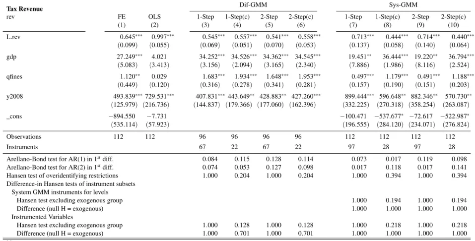
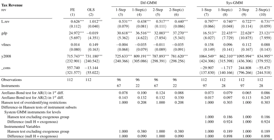
In this section, we present two tables with estimation results for our main model specification. We have also estimated coefficients for several other specifications as a way to test the robustness of the results. They are reported in the appendix and reveal that the main findings of the paper are robust to variations in the model specification.

The two tables here presented differ only by the fact that the first one treats the enforcement variables as endogenous. Therefore, in this case the lag of tax revenue, the quantity and the value of issued fines are instrumented with their own lagged values. In the second table, only the lag of tax revenue receives such treatment.

Columns (1) and (2) are the same in both tables. They contain estimates generated using Fixed Ef-fects (FE) and Pooled OLS methods. The FE results are used as a lower bound reference for the GMM estimates. OLS results are reported but not used in the analysis since its values do not seem to make sense when compared with the other estimation results. For example, the OLS autoregressive coefficient of tax revenue is bigger than 1, indicating the unlikely result that the tax revenue series would grow to in-finity in the long-run. The OLS coefficient of GDP, on the other hand, has a negative non-significant sign.

Results from tables 1.6 and 1.7 are similar. Both reveal that the autoregressive component of tax re-venue, the GDP, and tax enforcement are relevant determinants of tax rere-venue, both in terms of statistical significance and on the magnitude of the estimated coefficients. Most of the coefficients fulfil the FE lower bound requirement, with the exception of the ones on the lagged tax revenue variable and a few other cases. The coefficient on the quantity of issued fines is statistically significant in almost all situa-tions, whereas the total value of fines tend to impact positively the level of tax revenue through its first and second lagged values only. The current value of issued fines impact on tax revenue is neglectable and not statistically significant across specification and estimation models. This result is in line with the fact that current revenues from ICMS fines are, indeed, very small.

(27)

(7) and (9), the number of instruments is even higher than the number of observations. The lost in effi-ciency in these cases may be responsible for results which bear little in common with those of the other estimation techniques that do not face the same problem. In these cases, most of the estimated coeffi-cients are not statistically significant. The lag of tax revenue coefficient is considerably higher and the coefficient on the GDP is considerably lower than those found in other cases.

Hansen and Difference-in Hansen tests validate results in all but the instrument collapsed estimates of table 1.7. Within the same estimation technique, estimated coefficients vary little between instrument collapsed and non-collapsed versions.

Using the FE results as reference, it appears that difference GMM performs better. Within this class of estimators, we have selected 3 models which passed the lower bound “test” (two on table 1.6 and one on table 1.7). Those results are marked with bold letters in their respective tables. Specifically in these cases, instruments count is small when compared with the number of available observations, and test statistic support the models.

In what follows, we will interpret the results based on models and estimation methods of column (3), from table 1.7, combined with columns (4) and (6), from table 1.6. Except for the impact of the number of issued fines, estimated coefficient look very similar between these two specifications.

Persistence

Lagged tax revenue (“L.rev”) reveals a large degree of persistence. Its value is close to 0.45, implying

that the long run effect of the other tax revenue determinants are 1.8 times their short run effects.

Regional Income

As expected, the impact of the regional GDP variable (“gdp”) on tax revenues is positive and

statis-tically significant in all methodologies, except in (7) and (9) of table 1.6, in which the instruments count is higher than the number of observations. An increase of R$1 billion in the level of regional GDP raises ICMS revenues by R$38.19 millions (table 1.7(3)) and by R$38.41 millions(table 1.6(4)).

Quantity of Fines

Regardless of the specification and estimation method, except again for the (7) and (9) of table 1.6,

the coefficients on the quantity of fines issued (“qfines”) are positive and significant in all methodologies.

(28)

15

Tax Revenue Dif-GMM Sys-GMM

rev FE OLS 1-Step 1-Step(c) 2-Step 2-Step(c) 1-Step 1-Step(c) 2-Step 2-Step(c)

(1) (2) (3) (4) (5) (6) (7) (8) (9) (10)

L.rev 0.573∗∗∗ ₁_.₀₁₄∗∗∗ ₀_.₅₂₆∗∗∗ ₀_.₄₉₃∗∗∗ ₀_.₅₁₁∗∗∗ ₀_.₄₈₆∗∗∗ ₀_.₇₉₁∗∗∗ ₀_.₅₁₁∗∗∗ ₀_.₇₃₇∗∗∗ ₀_.₅₈₅∗∗∗

(0.114) (0.044) (0.103) (0.076) (0.097) (0.059) (0.129) (0.165) (0.162) (0.158)

gdp 30.744∗∗∗ ₋₁_.₆₄₁ ₃₄_.₃₉₃∗∗∗ ₃₈_.₄₁₁∗∗∗ ₃₉_.₃₁₂∗∗∗ ₃₇_.₀₅₇∗∗∗ ₁₀_.₇₆₃ ₃₂_.₉₅₇∗∗∗ ₁₆_.₉₆₇ ₃₁_.₇₁₄∗∗∗

(4.959) (5.972) (4.567) (5.360) (5.934) (4.236) (8.270) (6.151) (10.579) (6.884)

qfines 1.357∗∗∗ ₋₀_.₀₆₈ ₁_.₅₆₅∗∗∗ ₂_.₂₅₆∗∗∗ ₁_.₇₀₁∗∗∗ ₁_.₇₅₇∗∗∗ ₀_.₁₇₈ ₀_.₈₈₇∗∗∗ ₀_.₃₇₄ ₀_.₉₉₉∗∗∗

(0.452) (0.073) (0.391) (0.266) (0.537) (0.540) (0.154) (0.129) (0.429) (0.255)

vfines 0.023 0.187 −0.001 0.036 −0.080 0.005 0.143 −0.161 0.025 −0.239

(0.090) (0.206) (0.078) (0.122) (0.206) (0.060) (0.186) (0.115) (0.245) (0.190)

L.vfines 0.081 0.001 0.088 0.166∗ ₀_.₀₄₄ ₀_.₁₁₁∗∗ ₀_.₀₄₉ ₋₀_.₀₄₁ ₋₀_.₀₁₆ ₋₀_.₁₁₃

(0.087) (0.035) (0.084) (0.086) (0.136) (0.050) (0.072) (0.106) (0.163) (0.133)

L2.vfines 0.189 0.105 0.195 0.243 0.148 0.180∗ ₀_.₁₈₃ ₀_.₁₆₂ ₀_.₁₂₇ ₀_.₀₆₅

(0.179) (0.104) (0.169) (0.170) (0.267) (0.104) (0.160) (0.172) (0.290) (0.203)

y2008 430.302∗∗∗₇₁₉_.₂₅₂∗∗∗ ₃₉₀_.₂₄₂∗∗∗ ₃₄₈_.₂₉₀∗∗∗₄₂₄_.₆₃₀∗ ₆₉₆_.₅₁₁∗∗ ₇₆₈_.₆₈₄∗∗∗ ₆₉₁_.₁₂₅∗∗∗ ₆₉₆_.₀₆₃∗∗ ₅₀₉_.₆₄₉∗

(102.798) (227.238) (99.893) (127.812) (257.688) (350.602) (202.941) (208.971) (293.238) (289.183)

_cons −1391.093∗ ₋₉_.₃₁₆ ₋₄₃_.₅₈₅ ₋₂₃₈_.₃₈₃ ₋₁₃₇_.₀₂₂ ₋₃₂₇_.₂₉₀

(792.673) (67.374) (171.219) (267.394) (463.328) (757.027)

Observations 96 96 80 80 80 80 96 96 96 96

Instruments 67 22 67 22 97 28 97 28

Arellano-Bond test for AR(1) in 1st_diff. ₀_.₀₃₉ ₀_.₁₉₇ ₀_.₂₀₁ ₀_.₀₅₃ ₀_.₀₁₆ ₀_.₀₁₂ ₀_.₁₃₂ ₀_.₁₇₀ Arellano-Bond test for AR(2) in 1st_diff. ₀_.₀₆₅ ₀_.₀₉₃ ₀_.₁₀₃ ₀_.₀₁₂ ₀_.₆₂₆ ₀_.₁₀₆ ₀_.₈₃₉ ₀_.₂₆₅ Hansen test of overidentifying restrictions 1.000 0.877 1.000 0.877 1.000 0.942 1.000 0.942 Difference-in Hansen tests of instrument subsets

System GMM instruments for levels

Hansen test excluding exogenous group 1.000 0.654 1.000 0.654

Difference (null H = exogenous) 1.000 1.000 1.000 1.000

Instrumented Variables

Hansen test excluding exogenous group 1.000 0.772 1.000 0.772 1.000 0.888 1.000 0.888 Difference (null H = exogenous) 1.000 1.000 1.000 1.000 1.000 1.000 1.000 1.000 (a)_{Specifications (4), (6), (8), and (10) were obtained collapsing instruments in the weighting matrix}

(b)_{Standard errors in parentheses are robust and clustered by regions}

(c)_{For System-GMM, standard errors incorporate the Windmeijer (2005) correction} (d)_{For the test statistics, p-values reported}

(29)

Tax Revenue Dif-GMM Sys-GMM

rev FE OLS 1-Step 1-Step(c) 2-Step 2-Step(c) 1-Step 1-Step(c) 2-Step 2-Step(c)

(1) (2) (3) (4) (5) (6) (7) (8) (9) (10)

L.rev 0.573∗∗∗ ₁_.₀₁₄∗∗∗ ₀_.₄₁₉∗∗∗ ₀_.₃₅₉∗∗∗ ₀_.₄₃₃∗∗∗ ₀_.₄₇₅∗∗ ₀_.₄₈₉∗∗∗ ₀_.₃₂₅∗∗ ₀_.₄₄₁∗∗ ₀_.₃₅₄∗∗

(0.114) (0.044) (0.098) (0.091) (0.099) (0.206) (0.176) (0.145) (0.189) (0.172)

gdp 30.744∗∗∗ ₋₁_.₆₄₁ ₃₈_.₁₈₆∗∗∗ ₄₀_.₈₃₉∗∗∗ ₃₉_.₂₄₅∗∗∗ ₄₁_.₁₄₁∗∗∗ ₂₅_.₄₅₉∗∗ ₄₁_.₃₉₆∗∗∗ ₃₀_.₀₉₈∗∗∗ ₄₁_.₉₈₃∗∗∗

(4.959) (5.972) (4.162) (3.923) (6.248) (7.198) (10.782) (3.904) (10.474) (6.927)

qfines 1.357∗∗∗ ₋₀_.₀₆₈ ₁_.₃₈₀∗∗∗ ₁_.₁₅₈∗∗∗ ₀_.₉₉₇ ₀_.₆₉₂ ₀_.₅₉₆∗∗∗ ₀_.₉₄₃∗∗∗ ₀_.₂₉₁ ₀_.₉₆₂∗∗∗

(0.452) (0.073) (0.444) (0.429) (0.715) (1.153) (0.172) (0.130) (0.230) (0.163)

vfines 0.023 0.187 0.021 −0.003 −0.040 −0.071 0.090 −0.012 0.002 −0.007

(0.090) (0.206) (0.078) (0.068) (0.121) (0.145) (0.115) (0.049) (0.124) (0.070)

L.vfines 0.081 0.001 0.163∗∗ ₀_.₁₆₈∗∗ ₀_.₀₈₉ ₀_.₀₅₄ ₀_.₂₃₁∗∗∗ ₀_.₁₆₄∗∗ ₀_.₁₈₅∗∗∗ ₀_.₁₅₂∗∗

(0.087) (0.035) (0.074) (0.073) (0.101) (0.195) (0.054) (0.066) (0.065) (0.071)

L2.vfines 0.189 0.105 0.295∗ ₀_.₃₀₂∗ ₀_.₁₉₁ ₀_.₀₆₃ ₀_.₃₁₁∗∗ ₀_.₃₀₉∗ ₀_.₂₉₀∗ ₀_.₃₁₉

(0.179) (0.104) (0.152) (0.157) (0.176) (0.464) (0.155) (0.172) (0.168) (0.214)

y2008 430.302∗∗∗₇₁₉_.₂₅₂∗∗∗ ₃₉₈_.₁₆₃∗∗∗₄₇₅_.₁₈₅∗∗∗₅₂₃_.₀₆₃∗∗∗₄₉₀_.₉₈₂∗∗∗ ₆₇₅_.₇₄₃∗∗∗ ₅₁₀_.₄₁₁∗∗∗ ₇₅₂_.₁₃₀∗∗∗ ₄₈₈_.₅₄₃∗∗

(102.798) (227.238) (100.417) (113.747) (202.746) (158.041) (162.793) (149.549) (249.284) (211.218)

_cons −1391.093∗ ₋₉_.₃₁₆ ₋₂₁₈_.₅₃₀ ₋₅₃₆_._{841 1178}_.₆₅₃ ₋₄₂₄_.₄₁₅

(792.673) (67.374) (349.882) (338.939) (763.749) (447.345)

Observations 96 96 80 80 80 80 96 96 96 96

Instruments 26 12 26 12 33 14 33 14

Arellano-Bond test for AR(1) in 1st_diff. ₀_.₀₇₉ ₀_.₁₀₆ ₀_.₁₄₇ ₀_.₂₃₁ ₀_.₀₀₈ ₀_.₀₉₆ ₀_.₁₆₆ ₀_.₁₉₆ Arellano-Bond test for AR(2) in 1st_diff. ₀_.₁₆₇ ₀_.₁₄₂ ₀_.₁₆₇ ₀_.₈₀₉ ₀_.₄₂₅ ₀_.₂₄₁ ₀_.₅₇₄ ₀_.₄₈₅ Hansen test of overidentifying restrictions 0.962 0.091 0.962 0.091 0.997 0.042 0.997 0.042 Difference-in Hansen tests of instrument subsets

System GMM instruments for levels

Hansen test excluding exogenous group 0.878 0.099 0.878 0.099

Difference (null H = exogenous) 1.000 0.051 1.000 0.051

Instrumented Variables

Hansen test excluding exogenous group 0.553 . 0.553 . 0.945 . 0.945 . Difference (null H = exogenous) 1.000 . 1.000 . 1.000 0.042 1.000 0.042 (a)_{Specifications (4), (6), (8), and (10) were obtained collapsing instruments in the weighting matrix}

(b)_{Standard errors in parentheses are robust and clustered by regions}

(c)_{For System-GMM, standard errors incorporate the Windmeijer (2005) correction} (d)_{For the test statistics, p-values reported}

(30)

Value of Fines

As mentioned before, we expected that the effect of the value of issued fines on the level of ICMS revenues would be small in the short run. This is a stylized fact that can be explained by the existence of an administrative contention process, which allows penalized contributors to question the validity of

the fine. In all methodologies, the coefficients on the current value of fines issued (“vfines”) confirm our

thesis. They are all very small in magnitude and are not statistically significant.

Since the administrative contention process lasts 2 years, on average, and can be liquidated at any point in time by the fine payment, we would expect that at least part of the value of the fines issued were converted to revenues during this period. The coefficients on the first and second lagged values of fines

issued (“L.vfines”and“L2.vfines”) are, in general, positive and significant. For example, the impact of

of an additional billion Reais in issued fines (approximately 3.4% of the total value of issued fines in 2011), is R$163 millions in the first year and R$295 millions in the second, according to methodology (3) in table 1.7. With endogenous enforcement, the impact is smaller. Column (6) of table 1.6 reveals that the additional billion Reais would generate R$111 and R$180 millions in the first and second years, respectively.

Although it is not possible to affirm categorically that the effect on tax revenue of the lagged values of issued fines is derived directly from fines payment, we could say that, directly or indirectly, approxi-mately 45.8% (table 1.7(3)) or 29.1% (table 1.6(6)) of the additional billion Reais in the value of fines is converted in tax revenue during the length of the administrative contention process.

1.6 Conclusion

This paper analyses the effect of administrative enforcement actions on the level of revenue of a value-added tax, in a developing country environment. It employs data from the Brazilian state of São Paulo ICMS on the level of tax revenue and on two proxies for enforcement effort: the quantity and the total value of issued fines.

Controlling for the level of economic activity on a dynamic panel data setting, the paper results re-viled evidence that enforcement activities impact positively the level of tax revenues. At least in this specific environment, both the quantity and the total value of issued fines, this latter through is first and second lags, proved relevant variables both in terms of the statistical significance of the estimated coef-ficients and of the economic relevance of their impact.

(31)

1.7 Appendix: Additional Model Specifications

This section contains estimation results for several different model specifications. In all cases, tax revenue is a function of its lagged value and GDP. A dummy for the 2008 year is also include in all specifications. Specification 1 is the most parsimonious version. It contains no enforcement variables. Specification 2 is equal to specification 1 plus the quantity of fines. It has 2 versions, on with endogenous enforcement and the other with exogenous enforcement. Specifications 3 and 4 have the total value of issued fines as the enforcement variable. Specifications 5 and 6 include additional time dummies. Their composition follow the summary table below.

Tabela 1.8: Summary of Variables Employed on Different Specifications

Specification

Dep. Var. 1 2end 2exo 3end 3exo 4end 4exo 5end 5exo 6end 6exo

L.rev ✓ ✓ ✓ ✓ ✓ ✓ ✓ ✓ ✓ ✓ ✓

GDP ✓ ✓ ✓ ✓ ✓ ✓ ✓ ✓ ✓ ✓ ✓

y2008 ✓ ✓ ✓ ✓ ✓ ✓ ✓ ✓ ✓ ✓ ✓

qfines (endog)† _✓

qfines ✓

vfines (endog) ✓ ✓

vfines ✓ ✓

L.vfines (endog) ✓

L.vfines ✓