Using common features to understand the behavior of metal-commodity prices and forecast them at different horizons

(1)

Ensaios Econômicos

Escola de

Pós-Graduação

em Economia

da Fundação

Getulio Vargas

N◦ 735 ISSN 0104-8910

Using Common Features to Understand the

Behavior of Metal-Commodity Prices and

Forecast them at Diferent Horizons

João Victor Isslery, Claudia Rodrigues, Rafael Burjack

(2)

Os artigos publicados são de inteira responsabilidade de seus autores. As

opiniões neles emitidas não exprimem, necessariamente, o ponto de vista da

Fundação Getulio Vargas.

ESCOLA DE PÓS-GRADUAÇÃO EM ECONOMIA Diretor Geral: Rubens Penha Cysne

Vice-Diretor: Aloisio Araujo

Diretor de Ensino: Carlos Eugênio da Costa Diretor de Pesquisa: Humberto Moreira

Vice-Diretores de Graduação: André Arruda Villela & Luis Henrique Bertolino Braido

Victor Isslery, Claudia Rodrigues, Rafael Burjack, João Using Common Features to Understand the Behavior of Metal-Commodity Prices and Forecast them at Diferent Horizons/ João Victor Isslery, Claudia Rodrigues, Rafael Burjack – Rio de

Janeiro : FGV,EPGE, 2013

54p. - (Ensaios Econômicos; 735)

Inclui bibliografia.

(3)

Using Common Features to Understand the

Behavior of Metal-Commodity Prices and

Forecast them at Di¤erent Horizons

João Victor Issler

y

Claudia Rodrigues

z

Rafael Burjack

x

June 4, 2013

Abstract

The objective of this article is to study (understand and forecast) spot metal price levels and changes at monthly, quarterly, and annual horizons. Data consists of metal-commodity prices at a monthly and quarterly frequency from 1957 to 2012, extracted from the IFS. Annual data is provided from 1900-2010 by the U.S. Geological Survey (USGS). We also employ the (relatively large) list of co-variates used inWelch and Goyal(2008) and inHong and Yogo

(2009).

We gratefully acknowledge the comments and suggestions of Roberto Castello Branco, Robert Engle, Afonso Arinos de Mello Franco Neto, Allan Timmermann, the Editor in charge (Rabah

Arezki), …ve anonymous referees, and seminar participants at the 2013 IMF seminar on

Under-standing International Commodity Price Fluctuations and the 2012 VALE-EPGE conference on

The Economics and Econometrics of Commodity Prices. All remaining errors are ours. Issler thanks CNPq, FAPERJ and INCT for …nancial support. We thank Marcia Waleria Machado and Marcia Marcos for excellent research assistance.

y_{Graduate School of Economics - EPGE, Getulio Vargas Foundation. email:} _{[email protected]}

z_{Investor Relations Department, Vale. email:} _{[email protected]}

x_Graduate _School _of _Economics _- _EPGE, _Getulio _Vargas _Foundation _email:

(4)

We investigate short- and long-run comovement by applying the techniques and the tests proposed in the common-feature literature. Regarding out-of-sample forecasts, we use a variety of models (linear and non-linear, single equation and multivariate) and a variety of co-variates and functional forms to forecast the returns and prices of metal commodities. With the forecasts of a large number of models (N _{large) and a large number of time periods (}T

large), we apply the techniques put forth by thecommon-feature literature on forecast combinations.

The main contribution of this paper is to understand the short-run dy-namics of metal prices. We show theoretically that there must be a positive correlation between metal-price variation and industrial-production variation if metal supply is held …xed in the short run when demand is optimally chosen taking into account optimal production for the industrial sector. This is simply a consequence of the derived-demand model for cost-minimizing …rms. Our empirical evidence fully supports this theoretical result, with overwhelming evidence that cycles in metal prices are synchronized with those in industrial production. This evidence is stronger regarding the global economy but holds as well for the U.S. economy to a lesser degree.

Regarding forecasting, we show that models incorporating (short-run) common-cycle restrictions perform better than unrestricted models, with an important role for industrial production as a predictor for metal-price variation. Still, in most cases, forecast combination techniques outperform individual models.

1 Introduction

The purpose of this paper is twofold. The …rst is to improve our understanding of metal-commodity price variation either in the long run or in the short run by using standard time-series techniques. We rely on the common-trend and common-cycle

approach put forward by Engle and Kozicki (1993), Vahid and Engle (1993, 1997),

(5)

cyclical component, where their properties can be jointly investigated in a uni…ed multivariate setting based on vector autoregressive (VAR) models. Trends and cycles can be common to a group of series being modelled, and thesecommon features can be removed by independent linear combination1_{. Our second objective is to improve}

on current forecasts of metal-commodity prices taking into account the recent …nan-cialization of commodity markets and the role of information in commodity markets; see Hong and Yogo (2009, 2012) and Gargano and Timmermann (2012). Instead of relying on a speci…c model to forecast metal-commodity prices, we diversify out the risk of large forecast errors (and increase the information set used in forecast-ing) by combining forecasts of di¤erent models. This approach, …rst put forward by Bates and Granger (1969), has been shown to reduce forecast uncertainty in a variety of studies; see Hendry and Clements (2004) and Stock and Watson (2006). Recently, Issler and Lima (2009) have developed an optimal forecast-combination in a panel-data setting, where forecasts of di¤erent models (or survey results) com-prise the cross-sectional dimension. In their context, the optimal forecast using a mean-squared error (MSE) risk function can be consistently estimated employing the bias-corrected average forecast (BCAF), which is a common feature of all fore-cast models.

Early modern empirical work on commodity prices focused on the behavior of trend prices – Cuddington and Urzúa (1989) and Cuddington (1992). Trends are modelled as martingale processes. As (Deaton, 1999, p. 27) put it, referring to the drift term in commodity prices: “what commodity prices lack in trend, they make up for in variance.” Cashin et al. (2002) summarize the “stylized facts about real commodity prices: they are often dominated by long periods of doldrums punctuated by sharp upward spikes (Deaton and Laroque (1992)); they have a tendency to trend down in the long run (Grilli and Yang (1988)); shocks to commodity prices tend to persist for several years at a time (Cashin et al. (2000)); and unrelated commodity prices move together (Pindyck and Rotemberg (1990)).”

Despite the interest on the trends of commodity prices, little work has been done on cycles, the early exceptions being Labys et al. (1999), Cashin et al. (1999), and

(6)

Pindyck and Rotemberg(1990). Recently, however, there has been a renewed interest on commodity-price cycles, seeJerrett and Cuddington(2008) andIMF(2012). Our paper complements this recent e¤ort: while it investigates trends and cycles of metal commodities in an integrated way, its main focus is on metal-commodity cycles.

One of the main contributions of this paper is to understand the short-run dy-namics of metal prices. In the short run, we show theoretically that there must be a positive correlation between metal-price variation and industrial-production vari-ation if metal supply is held …xed when demand is optimally chosen taking into account optimal production for the industrial sector. This is simply a consequence of the derived-demand model for cost-minimizing …rms. The details of this models are given in Section 2. Our empirical evidence in Section 5 (monthly and quarterly data) fully supports this theoretical result, with overwhelming evidence that cycles in metal prices are synchronized with those in industrial production. This evidence is stronger regarding the global economy but holds as well for the U.S. economy to a lesser degree. As far as we know, we were the …rst authors to investigate and …nd common cycles in this way, accounting for theory and empirics, and not just describing a stylized fact2_.

Our second contribution is in forecasting metal prices at di¤erent horizons. In doing so, we try to incorporate the overwhelming evidence found on common cy-cles between metal prices and industrial production. One of the advantages of the

common-trend and common cycle method is parsimony, with obvious bene…ts for building e¢cient forecasting models; see Issler and Vahid (2001), Vahid and Issler

(2002), andAthanasopoulos et al. (2011). As is well known, vector autoregressions (VARs) have been increasingly used in multivariate analysis and in forecasting eco-nomic data. One of their shortcomings is the excessive number of parameters. For example, aV AR(p) for n series hasn2 _p _{parameters in the conditional mean. One}

can easily see the burden on degrees of freedom if the number of series being mod-elled (n) is large. Cointegration certainly reduces the number of parameters, but

2_{Obviuosly, we were not …rsts to investigate the cyclical behavior of metal prices (Jerrett and}

(7)

these reductions are mild. On the other hand, short-run restrictions – or common cycles – have a much greater potential to reduce the number of parameters in the dy-namic representation. For example, when dealing with post-war quarterly data, and a VAR with three variables and eight lags, there are seventy …ve mean parameters to be estimated from about two hundred data points on each variable. If the three-variable system has one known cointegrating vector, the number of free parameters falls from seventy …ve to sixty nine when estimating a vector error-correction model – VECM. Common-cyclical features show more potential in reducing the number of conditional-mean parameters. If the three variables in the VECM share one common cycle, then the number of mean parameters falls from sixty nine to twenty seven.

Using e¢cient models in forecasting metal prices is of obvious interest. However, most models are misspeci…ed, and it has been largely documented that the average forecast using several models outperforms individual models themselves; seeHendry and Clements (2004). Hence, we apply forecast-combination methods to forecast metal prices, showing that they work in practice. We go one step beyond, resorting to a common-feature technique proposed by Issler and Lima (2009).

Indeed,Bates and Granger(1969) made the econometrics profession aware of the bene…ts of forecast combination when a limited number of forecasts is considered. The widespread use of di¤erent combination techniques has lead to an interesting puzzle from the econometrics point of view – the forecast combination puzzle: if we consider a …xed number of forecasts (N <1), combining them using equal weights

(8)

(2009), with the added twist that now N; T ! 1, with T ! 1 prior thanN: the sequential asymptotic approach developed byPhillips and Moon (1999), denoted by

(T; N ! 1)seq.

Forecast combination works well in practice because of risk diversi…cation: idio-syncratic forecast errors vanish because of the WLLN works as the number of fore-casts being combined increases without bounds. However, the forecast combination puzzle also works against forecast combinations because of the curse of dimension-ality: as N increases, if one has to estimate “optimal weights” to combine forecasts with a …xed number of observations, the estimates of these weights are inconsistent. Issler and Lima solve the curse of dimensionality by imposing equal weights that need not be estimated(1=N), and perform bias correction to take MSE down to its minimum, identifying, in the limit, the conditional expectation of the series being forecast: if yt is the series being forecast, and h is the horizon, then, what is being

identi…ed is the latent variableEt h(yt), whereEt h( )is the conditional expectation

operator using all information available (observable or not) up to periodt h. Here, we are able to expand the information content of every individual model.

The paper is divided as follows: Section 2 presents a theoretical model that delivers common cycles among metal prices and industrial output. Sections 3 and 4 summarize the econometric techniques employed here, while the empirical results are reported in detail in Section 5. Section 6 concludes.

2 Understanding the Fluctuations of Metal-Commodity

Prices

(9)

“what commodity prices lack in trend, they make up for in variance.”Cashin et al.

(2002) summarize the “stylized facts about real commodity prices: they are often dominated by long periods of doldrums punctuated by sharp upward spikes (Deaton and Laroque(1992)); they have a tendency to trend down in the long run (Grilli and Yang(1988)); shocks to commodity prices tend to persist for several years at a time (Cashin et al.(2000)); and unrelated commodity prices move together (Pindyck and Rotemberg (1990)).”

Despite the proliferation of trend studies, the literature on the cyclical ‡uctua-tions of commodity prices has not been so proli…c. Indeed,Jerrett and Cuddington

(2008) note that “authors have analyzed the movement of metal prices over the busi-ness cycle as well as comovements among commodity prices (seeLabys et al. (1999);

Cashin et al.(1999); andPindyck and Rotemberg(1990)).” Regarding cycles,Deaton and Laroque (1996) is an important paper emphasizing the importance of demand shocks for short-run ‡uctuations. As they put it, “it is likely that demand shocks are a more plausible source of price ‡uctuations than has usually been supposed in the literature3_.”

As noted in the Introduction, we argue here that there is an important role for demand shocks in explaining the short-run variation of metal-commodity prices. In-deed, the overwhelming empirical evidence below suggests that the short-run ‡uctua-tions of metal-commodity prices are synchronized with those of industrial production in a global scale. To a lesser degree, they are also synchronized with U.S. industrial production. In trying to understand how these stylized facts come about, we devise a simple theoretical model motivated by the fact that metal commodities are in-puts in industrial production processes, which generates aderived demand for metal commodities.

Consider a representative industrial …rm, which chooses the optimal quantity of inputsxi,i= 1;2; ; n, all stacked in a vectorx= (x1; x2; ; xn)0, when producing

output y0. The choice of output y0 can be thought as an optimal decision coming

from the …rm’s output market. The corresponding prices for inputs i = 1;2; ; n,

3_{Recently, there has been a renewed interest on commodity-price cycles, see}_{Jerrett and}

(10)

stacked in a vector w = (w1; w2; ; wn)0, are considered given for the …rm when

choosingx. The …rm’s cost minimization problem in this context is:

min

x C(w; x) = w x s:t: f(x) y0: (1)

From the …rst-order (interior) condition of this problem, using Shepard’s Lemma, we derive the optimal derived demands for all inputs, labelledxi(w; y0):

@C(w; x )

@wi

=xi(w; y0); i= 1;2; ; n: (2)

A critical issue in describing the equilibrium for input markets is how to model supply. Of course, this depends on the horizon at which markets are supposed to clear. In modelling short-run ‡uctuations, it is reasonable to assume that metal-commodity supply cannot be increased without climbing a very steep cost function. Thus, we treat supply as …xed (xi) in the short run. This assumption is consistent

with the fact that mining projects are very intensive in capital and take a long time to mature. Since capital is traditionally held …xed in short-run analysis, this is similar to …xed short-run supply. Even if one considers the existence of inventories, they also cannot change in quantity in the short run. Indeed, we can think as the inventories as part of this …xed supply(xi) for metal commodities.

Thus, the short-run equilibrium condition for inputs (including metal commodi-ties) is:

xi(w; y0) =xi: i= 1;2; ; n: (3)

Ceteris paribus, given the equilibrium condition (3), we investigate how changes in output potentially change the price of input i, wi, considered here to be a metal

(11)

wi and in industrial production, y0, later solving for dw_dy0i:

0 = @xi(w; y0)

@wi

dwi+

@xi(w; y0)

@y0

dy0; or,

dwi

dy0 =

@x_i(w;y0)

@y0

@x_i(w;y0)

@wi

: (4)

It is straightforward to establish unequivocally that dwi

dy0 > 0 since, from

the-ory, we should have @xi(w;y0)

@y0 > 0 and

@x_i(w;y0)

@wi < 0. This result dwi

dy0 >0 is

completely intuitive: given concavity of the cost function vis-a-vis input prices

@x_i(w;y0)

@wi = @2_C

(w;x ) @w2

i <0 , if the representative …rm wants to increase industrial

production in the short run, it will put an upward pressure in the metal-commodity market, stemming from the fact that it should take more inputs to produce more

@x_i(w;y0)

@y0 >0 , otherwise it is not a cost minimizer.

In this setup, changes in industrial production have a positive correlation with changes in metal-commodity prices. Of course, this does not imply that these ‡uc-tuations will be synchronized, but that is the object of the empirical investigation in Section 5 below. It should also be noted that, as the equilibrium horizon becomes larger, supply cannot be treated as …xed, which reduces the importance of demand factors.

3 Cointegration and Common Cycles for Metal

Prices

(12)

Assume that yt is a n-vector of I(1) metal prices4 (or log metal prices), which

can be represented by a vector autoregression (VAR) model in levels:

yt= 1yt 1+: : :+ pyt p+ t: (5)

If elements of yt cointegrate, Engle and Granger (1987) showed that the system

(5) can be written as a Vector Error-Correction model (VECM):

yt = 1 yt 1+ : : : + p 1 yt p+1+ 0yt 1+ t (6)

where and are full rank matrices of ordern r,r is the rank of the cointegrating

space, I

p P i=1

i = 0, and j = p P i=j+1

i , j = 1; : : : ; p 1.

For our purposes, testing for cointegration will be used to verify whether metal-price data share common trends (or have long-run comovement). As is well known, metals are an important input in industrial processes, and thus it is expected that most metals would have their long-run prices linked to global industrial factors.

Testing for common trends among yt will use the maximum-likelihood approach

in Johansen (1991). A key issue to assure that inference is done properly is to estimate the lag length of the VAR (5) consistently, i.e., to estimate p consistently. Athanasopoulos et al. discuss how this can be achieved by using a combination of information criteria. An alternative to way to inferpis to perform diagnostic testing to rule out the risk of underestimation ofp, which leads to inconsistent estimates for the parameters in (6).

Vahid and Engle (1993) show that the dynamic representation for yt (6) may

be restricted if there exist white noise independent linear combinations of the series yt, i.e., if the yts share common cycles. These white noise linear combinations of

the series ytcan be expressed using cofeature vectors ~

0

i, stacked in ans nmatrix ~0, which eliminate all serial correlation in yt. Thus, ~0 yt = ~0 t. This is what

Hecq, Palm and Urbain (2006) have labelled strong-form serial-correlation common

4_{Other variables of interest may also be jointly modeled with metal-commodity prices, e.g.,}

(13)

features:

~0 ₁ = ~0 ₂ =: : := ~0 _p ₁ = 0, and (7)

~0 = 0: (8)

If we only impose restrictions (7), but not (8), we obtain what they have labelled

weak-form serial-correlation common features: ~0[ yt 0yt 1] = ~0 t, i.e., we

only inherit an unpredictable linear combination of yt once we control for the

long-run deviations 0_y

t 1 stemming from cointegration.

We continue the discussion of common cycles in the case of strong-form serial-correlation common features ((7) and (8)), given that the weak-form case can be immediately inferred from it5_{. Since cofeature vectors are identi…ed only up to an}

invertible transformation, without loss of generality, we can consider ~ to be of the form:

~ =

"

Is ~₍_{n s}₎ _s

#

Completing the system by adding the unconstrained VECM equations for the re-mainingn s elements of yt; we obtain a quasi-structural model,

2

4 Is ~ 0

0

(n s) s In s 3

5 yt = 2

4 s (np0+r) 1 : : : p 1

3 5 2 6 6 6 6 4

yt 1

... yt p+1

0_y t 1 3 7 7 7 7

5+vt: (9)

Since

2

4 Is ~ 0

0

(n s) s In s 3

5 is always invertible, we can recover (6) from (9).

How-ever, that the latter has s (np+r) s (n s) fewer parameters, thus, being over-identi…ed.

The literature on common cycles proposes estimation of the system in (9) in two di¤erent ways. The …rst is to employ full-information maximum likelihood (FIML),

(14)

constructing the likelihood function exploiting the correlation among the errors vt.

The other is to employ the generalized method of moments (GMM), exploiting the fact that the errors vt are orthogonal to the regressors in (9). Notice that this

includes the …rsts errors invt, which come from the white-noise combinations using ~. Analogously, testing for the existence of scofeature vectors – vectors leading tos linearly independent white noise combinations of the elements in yt – can be done

by canonical-correlation analysis (likelihood based) or by over-identifying-restriction tests (GMM based).

In testing for the existence of s serial-correlation common features (SCCF), by means of canonical-correlation analysis, the null hypothesis is that the …rst smallest s canonical correlations are jointly zero and the test statistic is T

s P i=1

log (1 i),

where i,i= 1; ; n, are the sample squared canonical correlations betweenf ytg

and f 0_y

t 1; yt 1; yt 2; ; yt p+1g. The limiting distribution of this test

sta-tistic is 2 _with _s₍_np₊_r₎ _s₍_n _s₎ _{degrees of freedom.}

One possible drawback of the canonical-correlation approach is that it assumes ho-moskedastic data, and that may not hold for metal-price (and other macroeconomic and …nancial data) collected at high frequency. In this case, a GMM approach is more robust, since inference can be conducted with Heteroskedastic and Auto-Correlation (HAC) robust estimates of the variance-covariance matrices of parameter estimates. The vector of instruments comprise the series in 0_y

t 1; yt 1; yt 2; ; yt p+1,

collected in a vector Zt 1. GMM estimation and testing exploits the following

mo-ment restriction:

0 ₌ _E_[_v_t _Z_t _{1] =} ₍₁₀₎

= E 2 6 6 6 6 4 0 B B B B @ 2

4 Is ~ 0

0

(n s) s In s 3 5 yt

2

4 s (np0+r) 1 : : : p 1

3 5 2 6 6 6 6 4

yt 1

.. . yt p+1

0_y t 1 3 7 7 7 7 5 1 C C C C

A Zt 1 3 7 7 7 7 5;

i.e., the orthogonality between all the elements invtand all the elements inZt 1. The

(15)

inHansen(1982) – which has an asymptotic 2 _{distribution with degrees of freedom}

equal to the number of over-identifying restrictions. The over-identifying restrictions test checks whether the errors of the system are orthogonal to all the instruments in Zt 1.

4 A Forecast-Combination Approach for Metal Prices

Here, we discuss the techniques used for optimal forecasting of metal-commodity prices. An in-depth theoretical discussion of these issues can be found inBates and Granger (1969), Palm and Zellner (1992), Stock and Watson (2006), Timmermann

(2006), and more recently in Issler and Lima (2009). The latter is our preferred approach here. It is appropriate for forecasting a weakly stationary and ergodic univariate process fytg using a large number of forecasts that will be combined to

yield an optimal forecast in the mean-squared error (MSE) sense. These forecasts are the result of several econometric models that need to be estimated prior to forecasting. We label forecasts of yt, computed using conditioning sets lagged h

periods, byfh

i;t, i = 1;2; : : : ; N . Therefore, fi;th are h-step-ahead forecasts and N is

the number of models estimated to forecastfh i;t.

Issler and Lima(2009) consider 3 consecutive distinct time sub-periods. The …rst sub-period E is labeled the “estimation sample”, where models are usually …tted to forecast yt subsequently. The number of observations in it is E = T1 = 1 T,

comprising (t = 1;2; : : : ; T1). The sub-period R (for regression) is labeled the

post-model-estimation or “training sample”, where realizations ofytare usually confronted

with forecasts produced in the estimation sample, and weights and bias-correction terms are estimated. It has R = T2 T1 = 2 T observations in it, comprising

(t =T1 + 1; : : : ; T2). The …nal sub-period is P (for prediction), where genuine

out-of-sample forecast is entertained. It has P = T T2 = 3 T observations in it,

comprising (t =T2+ 1; : : : ; T).

Forecasts fh

i;t’s are approximations to the optimal forecast (Et h(yt)) as follows:

fh

(16)

wherekh

i is the individual model time-invariant bias forh-step-ahead prediction and

"h

i;t is the individual model error term in approximating Et h(yt), where E("hi;t) = 0

for all i, t, and h. Here, the optimal forecast is a common feature of all individual forecasts and kh

i and "hi;t arise because of forecast misspeci…cation.

We can always decompose the series yt intoEt h(yt) and an unforecastable

com-ponent h

t, such that Et h( ht) = 0 in:

yt=Et h(yt) + ht: (12)

Combining (11) and (12) yields the well known two-way decomposition, or error-component decomposition, of the forecast errorfh

i;t yt:

fi;th = yt+ hi;t; i= 1;2; :::; N, and T > T1; (13) h

i;t = k h i +

h t +"

h

i;t, where h t =

h t

From the perspective of combining forecasts, the components kh

i, "hi;t and ht play

very di¤erent roles. If we regard the problem of forecast combination as one aimed at diversifying risk, i.e., a …nance approach, then, on the one hand, the risk associated with "h

i;t can be diversi…ed, while that associated with ht cannot. On the other

hand, in principle, diversifying the risk associated withkh

i can only be achieved if a

bias-correction term is introduced in the forecast combination, which reinforces its usefulness.

Issler and Lima propose the following non-parameteric consistent estimates for the componentskh

i,Bh, ht, and"hi;t: bkih = R1 PT2

t=T1+2f

h i;t R1

PT2

t=T1+2yt,Bc

h ₌ 1 N

PN i=1bkhi, bh

t = N1 PN

i=1fi;th Bch yt, b"i;th =fi;th yt bkhi bht. They show that, under a set

of conditions, thefeasible bias-corrected average forecast (BCAF) 1 N

PN

i=1fi;th Bch

obeys:

plim (T;N!1)seq

1

N

N X

i=1

fi;th Bch !

=yt+ ht =Et h(yt);

whereplim₍T;N!1)seq is the probability limit using the sequential asymptotic

(17)

device.

They also show that there is an in…nite number of optimal forecast combina-tions using deterministic weights f!igNi=1,such that !i 6= 0, !i = O(N 1)

uni-formly, with PN_i₌₁!i = 1 and limN!1PNi=1!i = 1. This allows the discussion

of the well-knownforecast combination puzzle: if we consider a …xed number of fore-casts (N <1), combining them using equal weights (1=N) fare better than using “optimal weights” constructed to outperform all other forecast combination in the mean-squared error (MSE) sense. Optimal population weights, constructed from the variance-covariance structure of models with stationary data, are optimal. Thus, the forecast-combination puzzle must be a consequence of the lack of consistency in estimating them, and can arise when N, the number of models being combined, is high relative to the number of observations used in estimating them by OLS –R.

Finally, there is one interesting case in which we can dispense with estimation in combining forecasts: when the mean bias is zero, i.e., Bh _{= 0}_{, there is no need to}

estimateBh _{and the BCAF is simply equal to} 1 N

PN

i=1fi;th, the sample average of all

forecasts. This is the ultimate level of parsimony. To test the null thatBh _{= 0}_{, Issler}

and Lima developed a robust t-ratio test that takes into account the cross-sectional dependence inkh

i.

4.1 Forecast Combination for Nested Models

The potential problem of nested models is that the innovations from nested models can exhibit high cross-sectional dependence, preventing a weak law-of-large numbers (WLLN) to hold. We introduce nested models by considering a continuous set of models splitting the total number of models N into M classes (or blocks), each of them containing m nested models, so that N = mM. In the index of forecasts, i= 1; : : : ; N, we group nested models contiguously. Hence, models within each class (block) are nested but models across classes (blocks) are non-nested.

The number of classes and the number of models within each class to be functions of N, respectively as follows: M = N1 d _and _m ₌ _Nd_{, where} ₀ _d ₁_{. Notice}

(18)

which all models are non-nested; d = 1 corresponds to the case in which all models are nested and; (iii) the intermediate case 0 < d < 1 gives rise to N1 d _{blocks of}

nested models, all with sizeNd_.

Regarding the interaction across blocks of nested models, it is natural to impose that the correlation structure of innovations across classes is such that it does not prevent a weak law-of-large numbers (WLLN) to hold, although we expect it not to hold within every block of nested models. Keeping some nested models poses no problem, since the mixture of all models will still deliver the optimal forecast. From a practical point of view, the choice of 0 d < 1 seems to be superior and is su¢cient to guarantee optimality of forecasts combinations as before.

5 Empirical analysis

5.1 Data and Empirical Implementation

We employed data of di¤erent frequencies and di¤erent sources building a very com-prehensive dataset of metal prices and potential co-variates that can be used either in building economics models and/or for forecasting. We have a library of data on three di¤erent frequencies: monthly, quarterly and annual.

(19)

and Yogo (2012), available from 1965 to 2008. This list includes: global, U.S., and Chinese industrial production, the primary metals coincident and leading indices, provided by the United States Geological Service (USGS), and a few …nancial-sector co-variates, such as: VIX – a volatility index, the U.S. real e¤ective exchange rate, returns and excess returns on U.S. government bonds at di¤erent maturities, and the return on the S&P500 index.

On a quarterly basis, the price data are for the same metals (or derived products) listed for monthly frequency. They are available from 1957:1 through 2012:1, and were extracted from IFS database. Nominal price data were de‡ated using the CPI for the U.S. We also employed the (relatively large) list of co-variates used inWelch and Goyal(2008) and inHong and Yogo (2012).

On an annual basis, metal-price data were provided by the United States Geo-logical Service (USGS), from 1900 through 2010. Annual prices were de‡ated by the U.S. CPI – a series put together by the St. Louis and Minneapolis Federal Reserve Economic Database. Actual annual CPI data covers the period 1913-2010, whereas the period 1900-13 uses FED estimates. We also employed the list of annual co-variates used in Welch and Goyal (2008) and in Hong and Yogo (2012) and a list of …nancial indices and real economic variables, such as Angus Maddison’s historical GDP, and Shiller’s U.S. per capita real consumption.

Our analysis of common-cyclical features will focus on the GMM tests proposed in Section 3, which is an appropriate testing strategy under unknown heterogeneity and dependence of the moment restrictions in question, which ultimately depend on these same features regarding the data being used. The same is not true for canonical-correlation analysis, therefore, we will not present it here in this version of the paper.

(20)

quarterly data are only available since 1957 (55 years of data), cointegration results using annual, quarterly and monthly data may not necessarily match. This may be simply a consequence of the fact that the samples used in these analyses are di¤erent. Regarding the forecasting exercise, the focus will be on monthly and annual frequencies alone – the former being appropriate to short-term forecasts and the latter to long-term forecasts.

5.2 Bivariate Analysis: Cointegration and Common Cycles

for Metal Prices

5.2.1 Monthly Frequency

Data for (log) prices of metals (or derived products) – Aluminium, Copper, Lead, Nickel, Tin and Zinc – are available from 1957:01 through 2012:03, whereas data for (log) Global Industrial Production (seasonally adjusted) is available from 1992:01 through 2012:09. Data for U.S. industrial production is available from 1919:1 on-wards. All these series show signs of containing a unit root, which is con…rmed for all of them using Phillips and Perron (1989) test6_.

First, we analyze the pairwise behavior of metal commodity prices alone, asking whether they share common trends and/or common cycles. Results are presented in Table 1. Regarding cointegration, we …nd overwhelming evidence of common trends among pairwise prices (10 out of 15). Conditional on this evidence, we tested for common cycles using the GMM approach (robust to heteroskedasticity and serial correlation of unknown form), …nding no signs of pairwise common cycles for the growth rates of metal-commodity prices – the only exception being the pair aluminum and lead, albeit the evidence is faint.

Next, we investigate whether prices for metal commodities cointegrate and/or share common cycles with global industrial production. The analysis is pairwise, one

6_{A slight caveat involves (log) aluminium prices, which rejects the null of a unit root at 5%}

(21)

commodity price at a time. Results are presented in Table 2 (panel A). Regarding cointegration, with the exception of aluminium, we …nd no evidence of a long-run relationship between metal prices and global industrial production for the last 20 years. On the other hand, results for common cycles are very di¤erent. Using the GMM approach, at 5% signi…cance, we found evidence of strong-form common-cyclical features between industrial production and the following metals: copper, nickel, tin, and zinc. In addition to that, we also found evidence of weak-form

common-cyclical features between industrial production and aluminium.

To motivate the …ndings of common cycles between global industrial production and the real price of copper, nickel, tin, and zinc, we detail here the results for copper, a metal for which its price is known to be associated with economic activity – the conventional wisdom of …nancial and business-cycle analysts for a long time7_.

In Figure 1 below, we plot the growth rates of copper prices – labelled ln PCo t

– and the growth rates of global industrial production – labelled ln IPG

t , both

standardized (zero mean, unit variance).

7_{There is a large group of webpages advertising the relationship between the Dow Jones}

(22)

-5 -4 -3 -2 -1 0 1 2 3

92 94 96 98 00 02 04 06 08 10

Copper Prices Growth Rates (std) Global Ind. Prod. Growth Rates (std)

Figure 1: Standardized Growth Rates of Global Industrial Production and Copper Prices

Notice that both ln PCo

t and ln IPtG show signs of serial correlation, as

is apparent from Figure 1 above. However, using the Ljung-Box test at 10% signif-icance, our empirical results in Table 2 found that the following linear combination is white noise (unpredictable):

ln PCo

t 7:523

(1:50) ln IP G

t + 0:015

(0:006); (14)

with robust standard errors in parenthesis. This shows that ln PCo

t and ln IPtG

are synchronized and that ln PCo

t and ln IPtG share a common cycle. As we

(23)

copper in producing industrial output for the global economy when the supply of copper is held …xed in the short run.

Next, still in Table 2 panel A, we investigate whether or not the growth rates of metal-commodity prices are synchronized with U.S. industrial production. Since we want to compare results with the previous tests using global industrial production, we employ the same sample period in the analysis (1992:1-2012:3), noting that U.S. industrial production is available from 1919:1 onwards. For the U.S., using the J-statistic, we …nd clear evidence of synchronized growth rates for industrial production and aluminium, tin, and zinc. Regarding lead and copper, the evidence is not so clear. In any case, overall, the only statistically signi…cant combinations of growth rates are the ones involving aluminium and tin, respectively. Thus, the evidence regarding the U.S. economy is weaker than that of the global economy. If we apply the same tests using the whole sample – 1957:1-2012:3 – we …nd no evidence of common cycles at all; see panel B in Table 2.

It is interesting to contrast the evidence of common cycles between metal-commodity prices and global industrial production with that between the former and U.S. indus-trial production. As is well known, there is a recent migration of indusindus-trial activity from developed countries to emerging economies, especially China and India. Global industrial production is highly in‡uenced by the industrial production of these two countries, which may explain why it is synchronized with metal-commodity prices. On the other hand, developed countries such as the U.S. have witnessed a contin-ued decline of its industrial sector, which may explain why we did not …nd strong evidence of synchronicity of U.S. industrial production and metal-commodity prices.

5.2.2 Quarterly Frequency

(24)

although our quarterly results are even stronger – 14 out of 15 pairs versus 10 out of 15.

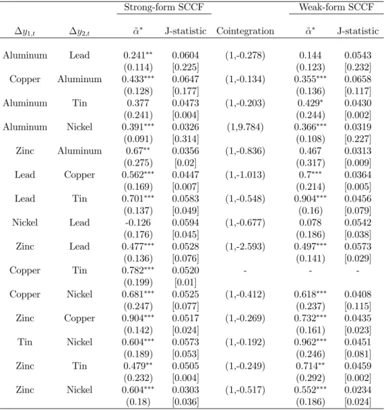
Regarding pairwise common cycles among commodity prices, we found limited evidence that they share common-cyclical features. Using the GMM approach de-scribed in Section 3, for all possible 15 pairwise cases, we found strong-form SCCF for 6 of them – aluminium-copper, aluminium-lead, aluminium-nickel, copper-nickel, lead-zinc, and nickel-tin. So, the growth rate of prices of aluminium and nickel are synchronized with those of other metal commodities. Similar results are also obtained for weak-form SCCF.

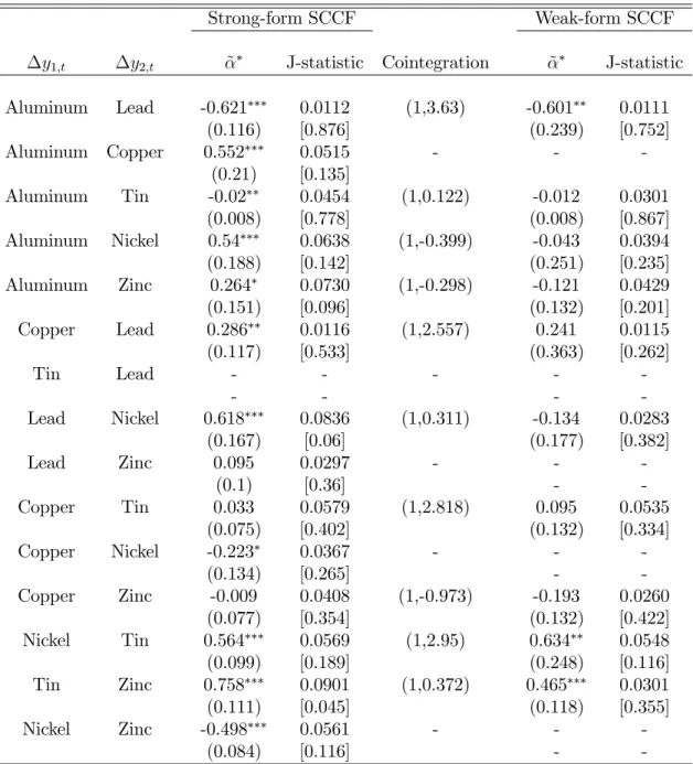
Next, using the sample 1992:1 through 2012:1, we investigate the existence of pairwise common trends and common cycles between metal-commodity prices and global and U.S. industrial production, respectively. Results are given in Table 4.

First, in panel A, we …nd no evidence of cointegration between metal prices and global and U.S. industrial production. Second, regarding global industrial production, we …nd strong evidence of common cycles for aluminium, copper, and tin. For zinc, there is a common cycle at 5% signi…cance, but not at 10%. Third, regarding U.S. industrial production, we …nd strong evidence of common cycles for aluminium only. For copper, tin, and zinc, there is a common cycle at 5% signi…cance, but not at 10%. Thus, we conclude that the evidence of common cycles is stronger regarding global industrial production. This result is consistent with our …ndings for the monthly frequency.

Finally, we investigate the existence of pairwise common trends and common cycles between metal-commodity prices and U.S. industrial production, using the complete sample from 1957:1 through 2012:1. Results are given in Table 4, panel B. In strong-form SCCF tests, we …nd hard evidence of common cycles for aluminium and nickel, and some evidence for lead and copper.

5.2.3 Annual Frequency

(25)

5 presents results of pairwise cointegration between metal prices. We found over-whelming evidence of cointegration between prices of di¤erent metal commodities. Given the longer span of this annual database vis-a-vis the monthly and quarterly databases – more than twice as long – cointegrating evidence here should receive more weight vis-a-vis previous evidence. From all possible 15 cases, we found cointegration among 10 pairs of metal-commodity prices.

One interesting issue is the long-run behavior of real metal-commodity prices: while three of them displayed an obvious increase in prices (copper, nickel, and zinc) in 110 years – more than a twofold increase from 1900 to 2010 – the other three displayed an obvious decrease over time (aluminium, lead, and tin) of about 70%-90%. We conjecture here that the industrial processes of the beginning of the 20th Century used aluminium, lead, and tin in larger quantities than what was used by the end of the 20th Century. An inverse pattern being observed for copper, nickel, and zinc.

As we stressed above, cointegration analysis requires the use of long-span data. Higher frequency at the expense of span is not a substitute for the latter. Thus, our preferred results are the ones obtained in cointegration tests when using annual data, given it has the longest span – 110 years of data. Monthly and quarterly data are only available since 1957 (55 years of data) – half the span of annual data. Notice that cointegration results for annual data may not necessarily match those for monthly or quarterly data. This may be simply a consequence of the fact that the samples used in these analyses are di¤erent: 1900-2010 versus 1957-2012.

(26)

period for the annual analysis.

Finally, we investigated whether there are cointegration and common cycles for metal prices and (U.S. or global) industrial production. Unfortunately the instanta-neous growth rates U.S. and global industrial production showed no signs of possess-ing a serial-correlation feature, which is a necessary condition to test for common cycles. Thus, we refrained here to go any further on that regard8_.

5.3 Multivariate Analysis: Cointegration and Common

Cy-cles for Metal Prices

We condition on previous evidence of bivariate cointegration and common cycles among metal prices and among metal prices and industrial production to build mul-tivariate models for (log) metal prices (or derived products) – Aluminium, Copper, Lead, Nickel, Tin and Zinc – and industrial production – either for the U.S. econ-omy or at a global level. We expect these multivariate models to display common cycles, so we construct two di¤erent sets of vector autoregressive (VAR) models to serve as reduced forms: one for metal prices and global industrial production and one for metal prices and U.S. industrial production – both with seven variables – later investigating if they possess common trends using Johansen’s (1991) test and common-cyclical-feature restrictions using the GMM approach of Section 3.

We focus on monthly data, since data at the highest frequency represent best the short-run analysis which are the object of theoretical modelling of Section 2 and the empirical evidence above. We were careful in selecting the lag order of the VAR to avoid having “dynamically incomplete” models; see Vahid and Issler (2002) and Athanasopoulos et al. (2011)9_{. For monthly data and global industrial production,}

we selected a VAR with two lags in levels. There is no evidence of cointegration

8_{This has some implications for the implementation of the optimal forecast methods discussed}

above, the main one being that we would not be able to build restricted VECMs (with common-cycle restrictions) to be later used in forecast combinations. Notice that, for the monthly frequency, we can do just that, linking theunderstanding part of this paper with theforecast part.

9_{Indeed, these papers document that using standard information criteria underestimates lag}

(27)

when all metal prices and global industrial production are jointly modelled. We selected …ve lags when U.S. industrial production was used instead, …nding again no cointegration for the system.

Next, we present GMM tests for common-cyclical-feature restrictions in the two systems described above. Results are presented in Table 6. We conclude for the existence of six cofeature vectors in both cases. Thus, all metal prices share a common cycle with industrial production (U.S. or global), given the form the contemporaneous relationships have in (6). This is consistent with our previous bivariate results, although a bit stronger, since, for the former, it was not unanimous.

To get an idea of the parsimony entailed by imposing common-cyclical-feature restrictions in a multivarite setting, note that the unrestricted VAR in di¤erences with one lag, such as (6), for six metal prices and global industrial production, has a total of 56 parameters. However, the same system where common-cyclical-feature restrictions are imposed (equation (9)) – with the existence of 6 cofeature vectors – has only 20 parameters. Testing whether it is valid to impose those restrictions leads to a p-value of 0.7376, which validates the restricted model at usual signi…cance levels10_.

To see this explicitly, denote by yt a vector stacking respectively the

instanta-neous growth rates of aluminium, copper, lead, nickel, tin zinc, and global industrial production, as shown in the right-hand-side of equation (15) below. The estimated

(28)

quasi-structural model took the form11_: 0 B B B B B B B B B B B @

ln PAL t ln PCo

t ln PP l

t ln PN i

t ln PT N

t ln PZn

t ln IPG

t 1 C C C C C C C C C C C A 7 1 = 2 6 6 6 6 6 6 6 6 6 6 6 6 6 6 6 6 6 4

1 0 0 0 0 0 7:023 (1:13) 0 1 0 0 0 0 2:13

(1:49) 0 0 1 0 0 0 6:87

(1:50) 0 0 0 1 0 0 5:45

(1:31) 0 0 0 0 1 0 9:60

(2:06) 0 0 0 0 0 1 8:13

(1:80)

0 0 0 0 0 0 1

3 7 7 7 7 7 7 7 7 7 7 7 7 7 7 7 7 7 5 1 (15) 2 4 0 6 7 0:02

(0:00) 0(0::002003) (00::002)005 0(0::004002) (00::004)008 0(0::008003) (00::1404)

3

5 yt 1;

As theory and experience has taught us, the restricted VECM forecasts much better than their unrestricted counterparts. In our previous experience, to give some idea of how much better the restricted VECM forecasts, consider the following: Issler and Vahid (2001) …nd a 25% reduction for the determinant of the mean-squared forecast error matrix – jM SP Ej – for U.S. macroeconomic aggregates, Vahid and Issler (2002) …nd a reduction of 20% for jM SP Ej when predicting U.S. coincident series using the same statistic, and Athanasopoulos et al. (2011) …nd a reduction of 47% for jM SP Ej when predicting di¤erent measures of Brazilian In‡ation.

Finally, in constructing the models that will be used in the forecast combination analysis, we will use some reduced-rank models where common cycles restrictions are imposed. Thus, our forecasts will bene…t from what we have learned in the empirical analysis regarding the synchronicity of cycles in metal-commodity prices and between the former and di¤erent measures of industrial production.

(29)

5.4 Forecasting Metal Prices using Forecast Combinations

We now implement the forecast theory discussed in Section 3 above, where forecast accuracy is measured by the root of the mean-squared forecast error. Metal-price data used here is the same one used in the cointegration and common-cycle analyses of the previous section, although we only focused on results for monthly and annual data alone. The former is appropriate to examine short-term forecast accuracy, whereas the latter is appropriate to measure long-term accuracy.

Our target variables in forecasting are commodity prices for Aluminium, Copper, Lead, Nickel, Tin and Zinc – made available from the London Mercantile Exchange (extracted from the IFS) for monthly frequency and from the USGS at annual fre-quency. For some of the estimated models, we used co-variates (predictors) which are highly correlated to metal prices. Some are related to economic activity, such as: the global industrial production, the U.S. industrial production, the Chinese industrial production, the primary metals coincident index (USGS), a leading index of metals price (USGS), and some other …nancial-sector co-variates, such as: VIX – a volatility index, the U.S. real e¤ective exchange rate and the S&P500 index.

Our monthly data set covers the period from January 1965 through December 2008, comprising 528 observations (T = 528). Our annual data set covers data from 1900 to 2010, comprising 111 observations (T = 111). Table 7 presents the correlations between the predictors are metal price data. Since there is evidence of a unit root for the metal prices and the co-variates used here, some series were transformed to instantaneous growth rates prior to computing correlations.

(30)

i.e., between115and125 distinct models and distinct forecasts for each time horizon (h). Obviously, some of them are nested within each other, and we also have classes of nested models as well. As we argued before, this will not pose as long as we have a large enough number of diverse classes.

For implementing the BCAF and other combining techniques discussed above, we split the sample in three distinct parts, each with a speci…c purpose: the …rst one, from1toT1, to estimate the coe¢cients of each model; the second fromT1+ 1toT2,

to compute the bias; and the third fromT2+1toT, to implement truly out-of-sample

forecasting, and to assess the forecast accuracy of di¤erent forecast strategies and of individual models using the root mean-squared error (RMSE) of forecasts.

To asses forecast accuracy, we constructed an algorithm which is appropriate for the bias-corrected average forecast (BCAF). For alternative forecast combinations or forecasting schemes, slight modi…cations are required. The algorithm runs as follows:

1. For each model (AR, VAR, VECM, restricted VECM with common-cycle re-strictions, and a speci…c set of predictors), we estimate the coe¢cients of the regressors using the sub-sample from1 toT1.

2. Forecasth-steps ahead the models estimated in step1(fh

it) fromT1 toT2. Each

model should be forecastedh-steps ahead T2 T1 h+ 1 times.

3. Calculate the bias associated with eachh-step ahead forecasts and each model; the bias is the average error between the h-steps ahead forecast and the ob-served value of the target series (fromT1 to T2).

4. Forecast h-steps ahead the same models estimated in step 1 for only T2 +h,

using the same coe¢cients estimated in step1.

5. Store the bias from step3 and the forecast made in step 4,fh i;T2+h.

6. Update T1 =T1+ 1, T2 =T2+ 1.

(31)

8. Adjust the forecasts of each model (made fromT2+ 1 toT) by their respective

bias.

9. Combine all these adjusted forecasts using equal weights.

10. Compute the RMSE of the BCAF, considering the series of metals price index as the target series.

For the monthly dataset, we took T1 = 200 and T2 = 378. Since T = 528, this

leaves 150 observations to evaluate out-of-sample performance of di¤erent models. For the annual data set, we took T1 = 35 and T2 = 70. Since T = 111, this leaves 41observations for out-of-sample evaluation. In both cases, we kept enough data to estimate the models and two similar-size sub-samples to estimate their biases and to perform out-of-sample forecasts.

The maximum horizon was set to 6months for monthly data and to6years with annual data. After computing the average bias for each forecast horizon (Bch_{), we}

tested the null H0 : Bh = 0, using Issler and Lima’s t-ratio test. Tables 8 and 9

present the results, respectively with monthly and annual data.

From the results in Tables 8and 9, we conclude that, for monthly data, none of the mean biases were signi…cant using the t-ratio test in Issler and Lima. For annual data, zinc is the only metal for which the mean bias is clearly non-zero. There is also scattered evidence of non-zero mean bias for copper and nickel at higher horizons.

Recall from Section 4 that, when the mean bias is zero, the optimal forecast collapses to the simple average across models 1

N PN

i=1fi;th. In this case, it might not

be worth discarding a part of the sample to compute the bias. Then, the best strategy is simply to merge the samplesE andRinto one (sample fromt= 1throught =T2),

where models are estimated.

5.4.1 Comparing forecast accuracy of di¤erent models

(32)

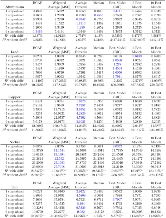
(WAF), where weights are based on the inverse of the mean-squared error for each model, normalized to add up to unity; (iv) the simple average (1=N) of the 5 best …tting models (by Bayesian Information Criteria – BIC, using a previous sample period); (v) the simple average (1=N) of the 10 best …tting models (BIC); (vi) the median forecast12_{. We computed the RMSE for these forecast strategies. Results are}

presented in Tables10 and 11, respectively for monthly and annual data. We could not make most forecast models for zinc to converge at the monthly frequency, and thus refrain from presenting its forecast-evaluation results.

For monthly data, for 1- through 6-steps ahead and across all metal prices, the best performance (by far) in terms of RMSE was achieved by the Average Forecast (AF), followed by the best model and then followed closely by the weighted average forecast (WAF). For 3 out of 5 metal prices, the Average Forecast (AF) was the best forecast strategy out of sample. This is exactly what one should expect from econometric theory (Section 4), given our evidence above that the average bias was statistically zero, i.e., that we could not reject the null H0 : Bh = 0, using Issler

and Lima’s t-ratio test in Table 8. Moreover, for 4 out of 5 metal prices, forecast combinations were superior to choosing a “best” model.

In Table 10, we also present out-of-sample R2 _{statistics (percentage) comparing}

forecast strategies with the random-walk model with and without drift, which are important benchmarks to be beaten in the …nance literature. R2_{-statistics were}

computed for one-step ahead forecasts only to save space. For metal price zt, we

have:

R2 = 100

2 6 6 6 6 6 4 1 T X

t=T2+1

zt bztjt 1 2

T X

t=T2+1

zt bz_tjtBM K₁ 2 3 7 7 7 7 7 5 ;

where _bztjt 1 is the one-step-ahead forecast of any given strategy and zbBM K_tjt ₁ is the

one-step-ahead forecast of the benchmark – random-walk with and without drift.

12_{For the median forecast, we have no theoretical optimality result. For the}₅_{-best and}₁₀_-best

(33)

For aluminium, copper and tin, our best strategy overall was the average forecast. It has R2 _{= 2}_:_75% _{for aluminium,} _R2 _{= 14}_:_30% _{for copper, and} _R2 _{= 14}_:_98% _for

tin, vis-a-vis the random walk with drift13_{. Table 10 also includes Clark and West’s}

(2007) tests for equal predictive accuracy applicable to nested models14_{. With the}

exception of nickel and tin, for all other models we cannot reject the null of equal forecast accuracy between any forecast strategy and the random-walk models.

For annual data, the best forecast strategy in terms of the RMSE is to employ the bias-corrected average forecast (BCAF) – for aluminium, lead and zinc, followed by average forecast (AF) – best for tin. Thus, for 4 out of 6 metal prices, forecast combinations were the best forecast strategy out of sample; see Table 11. In terms of out-of-sample R2 _{statistics, these best models outperformed the random walk with}

and without drift: R2 _{= 8}_:_59%_{for aluminium,}_R2 _{= 15}_:_90%_{for lead,}_R2 _{= 8}_:_98%_for

tin, andR2 _{= 23}_:_8% _{for zinc. Here, contrary to the evidence for monthly frequency,}

the best forecasts strategies are signi…cantly di¤erent (better) than the random walk using Clark and West’s test.

5.4.2 Best Predictors and Models used in Forecast Combinations

Tables 12 and 13 report, respectively, the best models and predictors for monthly and annual forecasts, considering out-of-sample results across all horizons. For each out-of-sample observation, and each forecast horizon, we compared models using squared forecast errors. The model with the smallest squared error is considered the best. Tables 12 and 13 report the percentage which each model type is considered best across all horizons and out-of-sample observations. Regarding predictors, notice that the models being combined are all autoregressive, so the lags of metal prices are used as predictors in them. The category no extra predictors includes only the these lags. For some models, we use extra predictors as well, which are also reported separately.

13_{Notice that, even when the average forecast was not the best strategy, it has beaten the random}

walk.

14_{Alquist, Kilian, and Vigfusson (2012) criticize Clark and West’s test, arguing that it rejects the}

(34)

For monthly frequency, the multivariate models – restricted vector error-correction models (VECM) described in Section 5.3 – with all metal prices and industrial pro-duction (U.S.), have the best forecasting performance overall. This connects “un-derstanding” and “forecasting,” both in the title of this paper. Moreover, it serves as empirical validation of the theoretical model discussed in Section 2 above, where demand for metals commodities are modelled as aderived demand in producing in-dustrial output and the supply of metal commodities are supposed to be …xed in the short run, due to the long maturity of metal-commodity projects and to their high capital intensity. The unrestricted VECMs also perform well, but not nearly as well as their restricted counterparts. Restricted and unrestricted VECMs highlight the importance of investigating short- and long-run relationships as done above.

The best predictors in monthly frequency are the lagged dependent-variables. This is expected, since most time-series models used here predict the future using the past and present. What is really informative is to look whichextra predictors do well out of sample. For monthly frequency, U.S. industrial production overwhelmingly outperforms all other predictors, with the S&P 500 and measures of realized volatility coming a far second for di¤erent metals.

For the annual frequency, we did not did not forecast using restricted common-cycle models (restricted VECMs), since U.S. industrial production has no serial cor-relation at that frequency. We were left with AR, VAR, and VECMs for forecasting metal prices. In this context, AR models were the best for aluminium and copper, VARs were best for lead and zinc, and VECMs were best for nickel and tin. For predictors, the best are lagged dependent-variables, as expected. In the class of ex-tra predictors, U.S. industrial production and volatility measures performed well for di¤erent metals.

6 Conclusion and Further Research

(35)

to 2012 extracted from the IFS. At annual frequency we use USGS data from 1900 through 2010. We also employ the (relatively large) list of co-variates used inWelch and Goyal(2008) and inHong and Yogo (2009) , which are available for download.

Regarding the understanding part of the paper, we were able to show theoret-ically that there must be a positive correlation between metal-price variation and industrial-production variation if metal supply is held …xed in the short run when its demand is optimally chosen taking into account optimal production for the in-dustrial sector. This is simply a consequence of the derived-demand model for cost-minimizing …rms, which is paramount in microeconomics (Section 2). Our empirical evidence (monthly and quarterly data) fully supports this theoretical result. Indeed, we have shown overwhelming evidence that cycles in metal prices are synchronized to those in industrial production. This evidence is stronger regarding the global economy but holds as well for the U.S. economy to a lesser degree. As far as we know, we were the …rst authors to investigate and …nd common cycles in this way, accounting for theory and empirics, and not just describing a stylized fact. This is one of the main contributions of this paper.

The second objective of the paper was to forecast metal prices in short horizons (monthly data) and in long horizons (annual data). We propose a novel technique which views the optimal forecast in the MSE sense as a common feature (latent variable), which can be identi…ed by using a cross-sectional average of a diverse group of forecasts, once we estimate a mean-bias term. There are several ways to combine forecasts optimally, but these combinations usually beat individual models. This was indeed our …nding, where combinations have beaten not only individual models most of the time but also the random walk model in several instances – which is usually not true for individual models. In predicting metal prices we connected the forecasting

andunderstanding parts of this paper by using several forecast models that imposed

common-cycle restrictions found in theunderstanding part15_{. We combined a variety}

of models (linear and non-linear, single equation and multivariate) and a variety of co-variates to forecast the returns and prices of six metal commodities. We found that the best performances in terms of RMSE were achieved by the average forecast

(36)

(AF), the bias-corrected average forecast (BCAF), and the weighted average forecast (WAF). These are all forecast-combination schemes, which achieve optimality by eliminating individual-model forecast error by means of the use of a weak law-of-large-numbers. These empirical results are true for most metal prices, frequencies, and horizons, although some individual models performed well on occasion.

Finally, we were able to identify which models and predictors had the best fore-cast performance for di¤erent metal prices. For monthly frequency, the multivariate models – restricted vector error-correction models (VECM) – with all metal prices and industrial production (U.S.), have the best forecasting performance overall. Best predictors are the U.S. industrial production, followed by the S&P 500 and measures of realized volatility coming a far second. For the annual frequency, the AR model, the VAR and the VECM performed well for di¤erent metal prices. The best predic-tors were the U.S. industrial production and volatility measures.

References

Alquist, Ron, Lutz Kilian, and Robert J. Vigfusson (2012). Forecasting the Price of Oil. Working Paper: University of Michigan.

Athanasopoulos, G., O. T. de Carvalho Guillén, J. V. Issler, and F. Vahid (2011). Model selection, estimation and forecasting in var models with short-run and long-run restrictions. Journal of Econometrics 164(1), 116 – 129.

Batchelor, R. (2007). Bias in macroeconomic forecasts. International Journal of Forecasting 23(2), 189 – 203.

Bates, J. M. and C. W. J. Granger (1969). The combination of forecasts. OR 20(4), pp. 451–468.

(37)

Cashin, P., H. Liang, and C. McDermott (2000). How persistent are shocks to world commodity prices? Working Paper: International Monetary Fund.

Cashin, P., C. McDermott, and A. Scott (1999). The myth of comoving commodity prices. Working Paper International Monetary Fund 99.

Cashin, P., C. McDermott, and A. Scott (2002). Booms and slumps in world com-modity prices. Journal of Development Economics 69(1), 277–296.

Chambers, M. J. and R. E. Bailey (1996). A theory of commodity price ‡uctuations.

Journal of Political Economy 104(5), pp. 924–957.

Clements, M. P. and D. F. Hendry (2006). Chapter 12 forecasting with breaks. Volume 1 of Handbook of Economic Forecasting, pp. 605 – 657. Elsevier.

Cuddington, J. (1992). Long-run trends in 26 primary commodity prices: A dis-aggregated look at the prebisch-singer hypothesis. Journal of Development Eco-nomics 39(2), 207–227.

Cuddington, J. and C. Urzúa (1989). Trends and cycles in the net barter terms of trade: a new approach. The Economic Journal 99(396), 426–442.

Davies, A. and K. Lahiri (1995). A new framework for analyzing survey forecasts using three-dimensional panel data. Journal of Econometrics 68(1), 205 – 227.

Deaton, A. (1999). Commodity prices and growth in africa.The Journal of Economic Perspectives 13(3), 23–40.

Deaton, A. and G. Laroque (1992). On the behaviour of commodity prices. The Review of Economic Studies 59(1), 1–23.

Deaton, A. and G. Laroque (1996). Competitive storage and commodity price dy-namics. Journal of Political Economy 104(5), pp. 896–923.

(38)

Engle, R. F. and C. W. J. Granger (1987). Co-integration and error correction: Representation, estimation, and testing. Econometrica 55(2), pp. 251–276.

Engle, R. F. and J. V. Issler (1995). Estimating common sectoral cycles. Journal of Monetary Economics 35(1), 83 – 113.

Engle, R. F. and S. Kozicki (1993). Testing for common features.Journal of Business and Economic Statistics 11(4), pp. 369–380.

Fuller, W. A. and G. E. Battese (1974). Estimation of linear models with crossed-error structure. Journal of Econometrics 2(1), 67 – 78.

Gargano, A. and A. Timmermann (2012). Predictive dynamics in commodity prices.

Working Paper.

Grilli, E. and M. Yang (1988). Primary commodity prices, manufactured goods prices, and the terms of trade of developing countries: what the long run shows.

The World Bank Economic Review 2(1), 1–47.

Hamilton, J. D. (2011). Nonlinearities and the macroeconomic e¤ects of oil prices.

Macroeconomic Dynamics 15, 364–378.

Hansen, L. P. (1982). Large sample properties of generalized method of moments estimators. Econometrica 50(4), pp. 1029–1054.

Hecq, A., F. Palm, and J. Urbain (2006). Common cyclical features analysis in var models with cointegration. Journal of Econometrics 132(1), 117–141.

Hendry, D. F. and M. P. Clements (2004). Pooling of forecasts. Econometrics Jour-nal 7(1), 1–31.

Hong, H. and M. Yogo (2009). Digging into commodities. Unpublished Working Paper, Princeton University and Wharton of University of Pennsylvania.

(39)

IMF (2012, April). World Economic Outlook: Growth resuming, dangers remain, Chapter 1, pp. 1–47. International Monetary Fund.

Issler, J. V. and L. R. Lima (2009). A panel data approach to economic forecasting: The bias-corrected average forecast. Journal of Econometrics 152(2), 153 – 164.

Issler, J. V. and F. Vahid (2001). Common cycles and the importance of transitory shocks to macroeconomic aggregates. Journal of Monetary Economics 47(3), 449 – 475.

Issler, J. V. and F. Vahid (2006). The missing link: using the nber recession indi-cator to construct coincident and leading indices of economic activity. Journal of Econometrics 132(1), 281 – 303.

Jerrett, D. and J. Cuddington (2008). Broadening the statistical search for metal price super cycles to steel and related metals. Resources Policy 33(4), 188–195.

Johansen, S. (1991). Estimation and hypothesis testing of cointegration vectors in gaussian vector autoregressive models. Econometrica 59(6), pp. 1551–1580.

Labys, W., A. Achouch, and M. Terraza (1999). Metal prices and the business cycle.

Resources Policy 25(4), 229–238.

Laster, D., P. Bennett, and I. Geoum (1999). Rational bias in macroeconomic fore-casts. The Quarterly Journal of Economics 114(1), 293–318.

Lettau, M. and S. Ludvigson (2001). Consumption, aggregate wealth, and expected stock returns. The Journal of Finance 56(3), 815–849.

Lettau, M. and S. C. Ludvigson (2004). Understanding trend and cycle in asset values: Reevaluating the wealth e¤ect on consumption. The American Economic Review 94(1), pp. 276–299.

(40)

Palm, F. C. and A. Zellner (1992). To combine or not to combine? issues of combining forecasts. Journal of Forecasting 11(8), 687–701.

Patton, A. and A. Timmermann (2007). Testing forecast optimality under unknown loss. Journal of the American Statistical Association 102(480), 1172–1184.

Phillips, P. C. B. and H. R. Moon (1999). Linear regression limit theory for nonsta-tionary panel data. Econometrica 67(5), pp. 1057–1111.

Pindyck, R. S. and J. J. Rotemberg (1990). The excess co-movement of commodity prices. The Economic Journal 100(403), pp. 1173–1189.

Stock, J. and M. Watson (2006). Forecasting with many predictors. Handbook of economic forecasting 1, 515–554.

Timmermann, A. (2006). Forecast combinations. In C. G. G. Elliott and A. Tim-mermann (Eds.), Handbook of Economic Forecasting, Volume 1 of Handbook of Economic Forecasting, pp. 135 – 196. Elsevier.

Vahid, F. and R. F. Engle (1993). Common trends and common cycles. Journal of Applied Econometrics 8(4), pp. 341–360.

Vahid, F. and R. F. Engle (1997). Codependent cycles. Journal of Economet-rics 80(2), 199 – 221.

Vahid, F. and J. V. Issler (2002). The importance of common cyclical features in var analysis: a monte-carlo study. Journal of Econometrics 109(2), 341 – 363.

Wallace, T. D. and A. Hussain (1969). The use of error components models in combining cross section with time series data. Econometrica 37(1), pp. 55–72.

Welch, I. and A. Goyal (2008). A comprehensive look at the empirical performance of equity premium prediction.The Review of Financial Studies 21(4), pp. 1455–1508.

(41)

Table 1: Common-Cycle Tests - Metal Prices (Monthly)

Strong-form SCCF Weak-form SCCF

y1;t y2;t ~ J-statistic Cointegration ~ J-statistic

Aluminum Lead -0.193 0.0118 - -

-(0.106) [0.05]

Copper Aluminum -1.15 0.0353 - -

-(0.029) [0.000]

Aluminum Tin -0.168 0.0130 - -

-(0.146) [0.035]

Nickel Aluminum -0.735 0.1407 - -

-(0.186) [0.000]