Essays in applied econometrics

(1)

FUNDAC

¸ ˜

AO GETULIO VARGAS

ESCOLA de P ´

OS-GRADUAC

¸ ˜

AO em

ECONOMIA

Rafael Burjack Farias Duarte

Essays in Applied Econometrics

(2)

Rafael Burjack Farias Duarte

Essays in Applied Econometrics

Tese submetida `a Escola de

P´os-Gradua¸c˜ao em Economia como

req-uisito parcial para a obten¸c˜ao do

grau de Doutor em Economia

´

Area de concentra¸c˜ao:

Econome-tria Aplicada

Orientador: Jo˜ao Victor Issler

(3)

Ficha catalográfica elaborada pela Biblioteca Mario Henrique Simonsen/FGV

Duarte, Rafael Burjack Farias

Essays in applied econometrics / Rafael Burjack Farias Duarte. – 2015. 128 f.

Tese (doutorado) - Fundação Getulio Vargas, Escola de Pós- Graduação em Economia.

Orientador: João Victor Issler. Inclui bibliografia.

1. Econometria. 2. Modelos econométricos. 3. Previsão econômica - Modelos econométricos. 4. Metais - Preço. I. Issler, João Victor. II. Fundação Getulio Vargas. Escola de Pós-Graduação em Economia. III. Título.

CDD – 330.0182

(4)

(5)

List of Figures

1.1 Standardized growth rates of global industrial production and copper prices 26

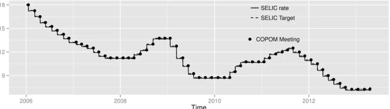
2.1 Evolution in the COPOM rateThe figure plots the time series of the COPOM rate

(step function) along with the effective SELIC market rate (solid line) over the period 1/1/2006 through 4/30/2013. . . 53

2.2 Distribution of changes to the COPOM rate This figure shows the distribution

of changes to the COPOM rate over the sample 1/1/2006-4/30/2013. All changes are

in units of 25 basis points. . . 54

2.3 Fixed event versus rolling event forecasts This figure compares the fixed event

forecasting format used in our paper (bottom diagram) to the more conventional format

with fixed horizon forecasts (top diagram). ˆyτi

t refers to the period-tforecast ofy at the first event following timet. In the figure, this event occurs after timet+ 1 as shown by the red lines. Hence the forecast horizon for ˆyτi

t is one period shorter than the forecast

horizon for ˆyτi

t+1. Event dates in our sample refer to the dates of COPOM meetings for

setting the COPOM rate and so are fixed. In the top diagram the forecast horizon is

fixed at two (green arrows) or three (purple arrows) periods. . . 56

2.4 Time series of survey forecasts The four graphs show time series of daily forecasts of GDP growth (top panel), inflation (second panel), the US dollar-Real exchange rate

(third panel) and the COPOM rate (bottom panel). The forecasts use the mean of the

daily surveys and assume a one-year forecast horizon. . . 58

2.5 Time series of dispersion in survey forecasts The four graphs show time series of the dispersion in the daily survey forecasts of GDP growth (top panel), inflation (second

panel), the US dollar-Real exchange rate (third panel) and the COPOM rate (bottom

panel). Each day the survey dispersion is measured as the cross-sectional standard

deviation of the survey forecasts. The time series assume a one-year forecast horizon. . 59

2.6 Actual versus predicted changes in the COPOM rate This figure plots actual

changes in the COPOM rate over the sample 1/1/2006 – 4/30/2013 against survey

forecasts of the change in the COPOM rate on the 59 meetings of the committee that

sets the interest rate target. . . 61

(6)

2.7 Time series of nominal and real bond yields The graphs show daily values of nominal (top panel) and real (bottom panel) bond yields for zero-coupon Brazilian

government bonds with maturities of 6, 9, 12, 18, 24, 36, and 48 months. . . 66

2.8 Loadings on principal components The figure plots the loadings of different bond maturities on principal components (PCs) extracted from nominal yields (left window)

and real yields (right window) using Brazilian government bonds with maturities ranging

from 6 through 48 months. . . 68

2.9 Time series of nominal short rates and term premiaThe top window plots daily

values of the observed one-year nominal yield along with the model-implied nominal rate

and expected short rates computed using a Gaussian dynamic term structure model

augmented with unspanned macro risk factors (JPS) or obtained from survey data. The

middle window plots the estimated nominal term premium implied by the Gaussian

dynamic term structure model with unspanned macro risk factors. Finally, the bottom

panel plots the nominal term premium computed from the survey expectations data,

T Psurvey ₌_{f r}₍₀_,₁₎ _rsurvey₍₀_,_{1), where} _{f r}₍₀_,_{1) is the forward rate from time zero} to time one (measured in years) and rsurvey₍₀_,_{1) is the survey forecast of the average} short rate over the next year. . . 72

2.10 Time series of real short rates and term premia The top window plots daily

values of the observed one-year real yield along with the model-implied real rate and

expected short rates computed using a Gaussian dynamic term structure model

aug-mented with unspanned macro risk factors or obtained from survey data. The

mid-dle window plots the estimated real term premium implied by the Gaussian dynamic

term structure model with unspanned macro risk factors. Finally, the bottom

win-dow plots the real term premium computed from survey expectations data,T Psurvey₌

f r(0,1) rsurvey₍₀_,₁₎₊_πsurvey₍₀_,_{1), where}_{f r}₍₀_,_{1) is the actual forward rate from time} zero to time one (measured in years),rsurvey₍₀_,_{1) is the survey forecast of the average} short rate over the next year, and πsurvey₍₀_,_{1) is the survey forecast of inflation over} the next year. . . 74

2.11 One-year realized and model-implied inflation rates The graph plots the

ob-served one-year inflation rate against the inflation rate implied by the Gaussian dynamic

term structure models fitted to real and nominal bond yields.. . . 77

2.12 One-day responses of short rates to expected and unexpected changes in

the COPOM rate . . . 79

2.13 One-day responses of real short rates to expected and unexpected changes

(7)

2.14 One-day responses of the term premium to changes in the COPOM rate These graphs show the one-day change in the nominal term premium (top panel) or the

real term premium (bottom panel) following a change in the COPOM rate on any of the

59 COPOM meeting dates during our sample 1/1/2006 - 4/30/2013. The left scatter

plots show the change in the term premium as a function of the actual change in the

COPOM rate; the middle and right diagrams plot the change in the term premia against

the expected and unexpected components of changes to the COPOM rate, along with

the best fitting linear model. The nominal and real term premia are computed from

dynamic Gaussian term structure models that include unspanned macro risk factors. . . 84

2.15 One-day responses of expected inflation and the inflation term premium

to changes in the COPOM rate These graphs show the one-day change in the

expected inflation (top panel) and the inflation term premium (bottom panel) following

a change in the COPOM rate on any of the 59 COPOM meeting dates during our sample

1/1/2006 - 4/30/2013. The left scatter plots show the change in the expected inflation

(top panel) or the inflation term premium (bottom panel) as a function of the actual

change in the COPOM rate; the middle and right diagrams plot the change in these

variables against the expected and unexpected components of changes to the COPOM

rate, along with the bet fitting linear model. The expected inflation and inflation term

premium are computed from Gaussian dynamic term structure models that include

unspanned macro risk factors. . . 86

2.16 Changes in two-year bond yields versus surprises in COPOM rates These

graphs plot the one-day change in the two-year nominal forward rate (left panel) or in

the average expected future short rate from time 0 to time 2 (years) against the surprise

component of the change in the COPOM rate following one of the 59 COPOM meeting

dates during our sample 1/1/2006 - 4/30/2013. . . 88

3.1 Consumption and national cash flow for selected countries - Real per capita

variables at 2005 prices . . . 112

(8)

(9)

List of Tables

1.1 Common-Cycle Tests - Metal Prices (Monthly) . . . 37

1.2 Common-Cycle Tests - Metal Prices and Industrial Production (Monthly) . 38 1.3 Common-Cycle Tests - Metal Prices (Quarterly) . . . 39

1.4 Common-Cycle Tests - Metal Prices and Industrial Production (Quarterly) 40 1.5 Common-Cycle Tests - Metal Prices (Annual) . . . 41

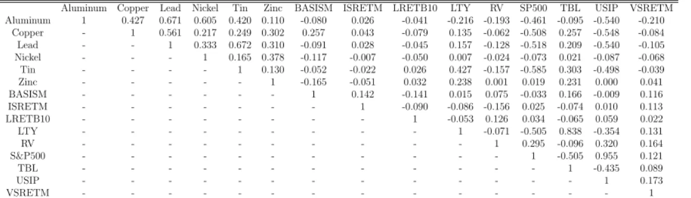
1.6 Multivariate Common-Cycle Test - Metal Prices and Industrial Production 42 1.7 Correlations Between the Metal Prices and Co-variates . . . 42

1.8 Mean Bias Significance Test (Monthly) . . . 43

1.9 Mean Bias Significance Test (Annual) . . . 44

1.10 Forecast Root-Mean-Squared-Error (Monthly) . . . 45

1.11 Forecast Root-Mean-Squarred-Error (Annual) . . . 46

1.12 Best Models and Predictors (Monthly) . . . 47

1.13 Best Models and Predictors (Annual) . . . 48

2.1 Survey variables . . . 55

2.2 Types of Brazilian government bonds . . . 62

2.3 Properties of principal components extracted from Brazilian bond yields . 67 2.4 Maximum likelihood estimates of the term structure model with unspanned macro risk factors . . . 70

2.5 Significance tests for unspanned macro factors . . . 71

2.6 Nominal and real forward term premia and dispersion in survey forecasts . 76 2.7 One-day response of interest rates, term premia, and inflation to expected and unexpected changes in the COPOM rate . . . 80

2.8 One-day responses of short rates, inflation expectations and term premia to alternative measures of unexpected changes in COPOM rate. . . 89

2.9 The Brazilian Term Structure One-day response to LSAP . . . 91

3.1 Panel Unit Root Tests . . . 113

3.2 Cointegration Tests - Consumption (ct) and net income (yt it gt) . . . 114

3.3 PVAR(p) Model Coefficients and statistics . . . 116

3.4 PVAR(p) Model Coefficients and statistics - Trade of freedom . . . 118

3.5 PVAR(p) Model Coefficients and statistics - High Income . . . 120

(10)

(11)

Chapter 1 Using Common Features to

Understand the Behavior of

Metal-Commodity Prices and

Forecast them at Di

_ff

erent Horizons

1.1 Introduction

The purpose of this paper is twofold. The first is to improve our understanding of metal-commodity price variation either in the long run or in the short run by using stan-dard time-series techniques. We rely on the common-trend and common-cycle approach put forward byEngle and Kozicki(1993),Vahid and Engle(1993,1997),Engle and Issler

(1995), Issler and Vahid (2001, 2006), Vahid and Issler (2002), Hecq et al. (2006), and

Athanasopoulos et al.(2011). Here, non-stationary economic series are decomposed into an integrated trend component and a stationary and ergodic cyclical component, where their properties can be jointly investigated in a unified multivariate setting based on vec-tor auvec-toregressive (VAR) models. Trends and cycles can be common to a group of series being modelled, and these common features can be removed by independent linear com-bination1_{. Our second objective is to improve on current forecasts of metal-commodity}

prices taking into account the recent financialization of commodity markets and the role of information in commodity markets; seeHong and Yogo(2009,2012) andGargano and Timmermann(2012). Instead of relying on a specific model to forecast metal-commodity prices, we diversify out the risk of large forecast errors (and increase the information set used in forecasting) by combining forecasts of different models. This approach, first put forward by Bates and Granger (1969), has been shown to reduce forecast uncertainty in a variety of studies; see Hendry and Clements (2004) and Stock and Watson (2006).

1_{Perhaps cointegration is the best-known example of}

common features.

(14)

Recently, Issler and Lima (2009) have developed an optimal forecast-combination in a panel-data setting, where forecasts of different models (or survey results) comprise the cross-sectional dimension. In their context, the optimal forecast using a mean-squared error (MSE) risk function can be consistently estimated employing the bias-corrected average forecast (BCAF), which is a common feature of all forecast models.

Early modern empirical work on commodity prices focused on the behavior of trend prices – Cuddington and Urz´ua (1989) and Cuddington (1992). Trends are modeled as martingale processes. As (Deaton, 1999, p. 27) put it, referring to the drift term in commodity prices: “what commodity prices lack in trend, they make up for in variance.”

Cashin et al.(2002) summarize the “stylized facts about real commodity prices: they are often dominated by long periods of doldrums punctuated by sharp upward spikes (Deaton and Laroque(1992)); they have a tendency to trend down in the long run (Grilli and Yang

(1988)); shocks to commodity prices tend to persist for several years at a time (Cashin et al. (2000)); and unrelated commodity prices move together (Pindyck and Rotemberg

(1990)).”

Despite the interest on the trends of commodity prices, little work has been done on cy-cles, the early exceptions beingLabys et al.(1999),Cashin et al.(1999), andPindyck and Rotemberg (1990). Recently, however, there has been a renewed interest on commodity-price cycles, seeJerrett and Cuddington(2008) andIMF(2012). Our paper complements this recent effort: while it investigates trends and cycles of metal commodities in an integrated way, its main focus is on metal-commodity cycles.

One of the main contributions of this paper is to understand the short-run dynamics of metal prices. In the short run, we show theoretically that there must be a positive cor-relation between metal-price variation and industrial-production variation if metal supply is held fixed when demand is optimally chosen taking into account optimal production for the industrial sector. This is simply a consequence of the derived-demand model for cost-minimizing firms. The details of this models are given in Section 2. Our empirical evidence in Section 5 (monthly and quarterly data) fully supports this theoretical result, with overwhelming evidence that cycles in metal prices are synchronized with those in industrial production. This evidence is stronger regarding the global economy but holds as well for the U.S. economy to a lesser degree. As far as we know, we were the first authors to investigate and find common cycles in this way, accounting for theory and empirics, and not just describing a stylized fact2_.

Our second contribution is in forecasting metal prices at different horizons. In doing so, we try to incorporate the overwhelming evidence found on common cycles between metal prices and industrial production. One of the advantages of the common-trend and

(15)

common cyclemethod is parsimony, with obvious benefits for building efficient forecasting models; see Issler and Vahid (2001), Vahid and Issler (2002), and Athanasopoulos et al.

(2011). As is well known, vector autoregressions (VARs) have been increasingly used in multivariate analysis and in forecasting economic data. One of their shortcomings is the excessive number of parameters. For example, aV AR(p) forn series hasn2_·_p_parameters in the conditional mean. One can easily see the burden on degrees of freedom if the number of series being modelled (n) is large. Cointegration certainly reduces the number of parameters, but these reductions are mild. On the other hand, short-run restrictions – or common cycles – have a much greater potential to reduce the number of parameters in the dynamic representation. For example, when dealing with post-war quarterly data, and a VAR with three variables and eight lags, there are seventy five mean parameters to be estimated from about two hundred data points on each variable. If the three-variable system has one known cointegrating vector, the number of free parameters falls from seventy five to sixty nine when estimating a vector error-correction model – VECM.

Common-cyclical features show more potential in reducing the number of conditional-mean parameters. If the three variables in the VECM share one common cycle, then the number of mean parameters falls from sixty nine to twenty seven.

Using efficient models in forecasting metal prices is of obvious interest. However, most models are misspecified, and it has been largely documented that the average forecast us-ing several models outperforms individual models themselves; seeHendry and Clements

(2004). Hence, we apply forecast-combination methods to forecast metal prices, show-ing that they work in practice. We go one step beyond, resortshow-ing to a common-feature

technique proposed by Issler and Lima(2009).

(16)

denoted by (T, N ! 1)seq.

Forecast combination works well in practice because of risk diversification: idiosyn-cratic forecast errors vanish because of the WLLN works as the number of forecasts being combined increases without bounds. However, the forecast combination puzzle also works against forecast combinations because of the curse of dimensionality: as N increases, if one has to estimate “optimal weights” to combine forecasts with a fixed number of observations, the estimates of these weights are inconsistent. Issler and Lima solve the curse of dimensionality by imposing equal weights that need not be estimated (1/N), and perform bias correction to take MSE down to its minimum, identifying, in the limit, the conditional expectation of the series being forecast: if yt is the series being forecast, and h is the horizon, then, what is being identified is the latent variableEt h(yt), where

Et h(·) is the conditional expectation operator using all information available (observable or not) up to period t h. Here, we are able to expand the information content of every individual model.

The paper is divided as follows: Section 2 presents a theoretical model that delivers common cycles among metal prices and industrial output. Sections 3 and 4 summarize the econometric techniques employed here, while the empirical results are reported in detail in Section 5. Section 6 concludes.

1.2 Understanding the Fluctuations of Metal-Commodity

Prices

From a theoretical point-of-view, commodity-price dynamics have been studied at least since Newbery and Stiglitz (1981),Deaton and Laroque(1992,1996) andChambers and Bailey (1996). Early modern empirical work on commodity prices has focused on the behavior of trend prices – Cuddington and Urz´ua (1989) and Cuddington (1992) – where trends were modelled as martingale processes. Regarding trends, as (Deaton,1999, p. 27) puts it, referring to the drift term in commodity prices: “what commodity prices lack in trend, they make up for in variance.”Cashin et al.(2002) summarize the “stylized facts about real commodity prices: they are often dominated by long periods of doldrums punctuated by sharp upward spikes (Deaton and Laroque (1992)); they have a tendency to trend down in the long run (Grilli and Yang (1988)); shocks to commodity prices tend to persist for several years at a time (Cashin et al. (2000)); and unrelated commodity prices move together (Pindyck and Rotemberg (1990)).”

(17)

(1999); and Pindyck and Rotemberg (1990)).” Regarding cycles, Deaton and Laroque

(1996) is an important paper emphasizing the importance of demand shocks for short-run fluctuations. As they put it, “it is likely that demand shocks are a more plausible source of price fluctuations than has usually been supposed in the literature3_.”

As noted in the Introduction, we argue here that there is an important role for de-mand shocks in explaining the short-run variation of metal-commodity prices. Indeed, the overwhelming empirical evidence below suggests that the short-run fluctuations of metal-commodity prices are synchronized with those of industrial production in a global scale. To a lesser degree, they are also synchronized with U.S. industrial production. In trying to understand how these stylized facts come about, we devise a simple theoretical model motivated by the fact that metal commodities are inputs in industrial production processes, which generates aderived demand for metal commodities.

Consider a representative industrial firm, which chooses the optimal quantity of inputs xi, i = 1,2,· · ·, n, all stacked in a vector x = (x1, x2,· · · , xn)0, when producing output

y0. The choice of outputy0 can be thought as an optimal decision coming from the firm’s output market. The corresponding prices for inputs i = 1,2,· · · , n, stacked in a vector w= (w1, w2,· · · , wn)0, are considered given for the firm when choosingx. The firm’s cost minimization problem in this context is:

min

x C(w, x) =w·x s.t. f(x) y0. (1.1)

From the first-order (interior) condition of this problem, using Shepard’s Lemma, we derive the optimal derived demands for all inputs, labelledx⇤

i(w, y0):

@C(w, x⇤

) @wi

=x⇤

i(w, y0), i= 1,2,· · ·, n. (1.2)

A critical issue in describing the equilibrium for input markets is how to model sup-ply. Of course, this depends on the horizon at which markets are supposed to clear. In modelling short-run fluctuations, it is reasonable to assume that metal-commodity supply cannot be increased without climbing a very steep cost function. Thus, we treat supply as fixed (xi) in the short run. This assumption is consistent with the fact that mining projects are very intensive in capital and take a long time to mature. Since capital is traditionally held fixed in short-run analysis, this is similar to fixed short-run supply. Even if one considers the existence of inventories, they also cannot change in quantity in the short run. Indeed, we can think as the inventories as part of this fixed supply (xi) for metal commodities.

Thus, the short-run equilibrium condition for inputs (including metal commodities)

(18)

is:

x⇤

i(w, y0) = xi. i= 1,2,· · · , n. (1.3)

Ceteris paribus, given the equilibrium condition (1.3), we investigate how changes

in output potentially change the price of input i, wi, considered here to be a metal commodity used in production. Totally differentiate (1.3) considering only changes in wi and in industrial production, y0, later solving for dw_dy0i:

0 = @x

⇤

i(w, y0) @wi

dwi+ @x⇤

i(w, y0) @y0

dy0, or,

dwi

dy0 =

∂x⇤

i(w,y0)

∂y0 ∂x⇤

i(w,y0)

∂wi

. (1.4)

It is straightforward to establish unequivocally that dwi

dy0 > 0 since, from theory, we should have ∂x⇤i(w,y0)

∂y0 >0 and ∂x⇤

i(w,y0)

∂wi <0. This result

⇣ dwi

dy0 >0

⌘

is completely intuitive:

given concavity of the cost function vis-a-vis input prices ⇣∂x⇤i(w,y0) ∂wi =

∂2 C(w,x⇤₎

∂w2

i <0

⌘

, if the representative firm wants to increase industrial production in the short run, it will put an upward pressure in the metal-commodity market, stemming from the fact that it should take more inputs to produce more ⇣∂x⇤i(w,y0)

∂y0 >0

⌘

, otherwise it is not a cost minimizer.

In this setup, changes in industrial production have a positive correlation with changes in metal-commodity prices. Of course, this does not imply that these fluctuations will be synchronized, but that is the object of the empirical investigation in Section 5 below. It should also be noted that, as the equilibrium horizon becomes larger, supply cannot be treated as fixed, which reduces the importance of demand factors.

1.3 Cointegration and Common Cycles for Metal Prices

We discuss here a unified econometric framework that allows investigating the exis-tence of short- and long-run restrictions for metal-commodity prices. An in-depth theo-retical discussion of these issues can be found in Engle and Granger (1987a), Vahid and Engle (1993), Vahid and Engle (1997), Hecq et al. (2006), and Athanasopoulos et al.

(2011).

Assume that yt is a n-vector ofI(1) metal prices4 (or log metal prices), which can be represented by a vector autoregression (VAR) model in levels:

yt =Γ1yt 1+. . .+Γpyt p+✏t. (1.5)

(19)

If elements ofytcointegrate, Engle and Granger (1987a) showed that the system (1.5) can be written as a Vector Error-Correction model (VECM):

∆yt=Γ

⇤

1∆yt 1+ . . . +Γ

⇤

p 1∆yt p+1+ ↵

0

yt 1+✏t (1.6)

where and ↵ are full rank matrices of order n⇥r, r is the rank of the cointegrating space, (I Pp_i₌₁Γi) = ↵0, and Γ⇤j =

Pp

i=j+1Γi , j = 1, . . . , p 1.

For our purposes, testing for cointegration will be used to verify whether metal-price data share common trends (or have long-run comovement). As is well known, metals are an important input in industrial processes, and thus it is expected that most metals would have their long-run prices linked to global industrial factors.

Testing for common trends among yt will use the maximum-likelihood approach in

Johansen(1991a). A key issue to assure that inference is done properly is to estimate the lag length of the VAR (1.5) consistently, i.e., to estimate p consistently. Athanasopoulos et al. discuss how this can be achieved by using a combination of information criteria. An alternative to way to infer p is to perform diagnostic testing to rule out the risk of underestimation ofp, which leads to inconsistent estimates for the parameters in (1.6).

Vahid and Engle (1993) show that the dynamic representation for yt (1.6) may be restricted if there exist white noise independent linear combinations of the series ∆yt, i.e., if the yts share common cycles. These white noise linear combinations of the series

∆yt can be expressed using cofeature vectors ˜↵ 0

i, stacked in an s⇥n matrix ˜↵

0

, which eliminate all serial correlation in∆yt. Thus, ˜↵0∆yt= ˜↵0✏t. This is what Hecq, Palm and Urbain (2006) have labelled strong-form serial-correlation common features:

˜ ↵0

Γ⇤

1 = ˜↵

0

Γ⇤

2 =. . .= ˜↵

0

Γ⇤

p 1 = 0, and (1.7)

˜ ↵0

= 0. (1.8)

If we only impose restrictions (1.7), but not (1.8), we obtain what they have labelled weak-form serial-correlation common features: ˜↵0

[∆yt ↵0yt 1] = ˜↵0✏t, i.e., we only inherit an unpredictable linear combination of ∆yt once we control for the long-run deviations ↵0

yt 1 stemming from cointegration.

We continue the discussion of common cycles in the case of strong-form serial-correlation common features ((1.7) and (1.8)), given that the weak-form case can be immediately inferred from it5_{. Since cofeature vectors are identified only up to an invertible}

transfor-mation, without loss of generality, we can consider ˜↵ to be of the form:

˜ ↵ =

"

Is ˜ ↵⇤

(n s)⇥_s #

(20)

Completing the system by adding the unconstrained VECM equations for the remaining n s elements of∆yt, we obtain a quasi-structural model,

2

4 Is ↵˜

⇤0

0

(n s)⇥s

In s 3

5∆yt= 2

4 s⇥(np0+r)

Γ⇤⇤

1 . . . Γ

⇤⇤ p 1 ⇤ 3 5 2 6 6 6 6 4

∆yt 1 ... ∆yt p+1

↵0

yt 1

3 7 7 7 7

5+vt. (1.9)

Since

2

4 Is ↵˜

⇤0

0

(n s)⇥s

In s 3

5is always invertible, we can recover (1.6) from (1.9). However,

that the latter hass ·(np+r) s· (n s) fewer parameters, thus, being over-identified. The literature on common cycles proposes estimation of the system in (1.9) in two different ways. The first is to employ full-information maximum likelihood (FIML), con-structing the likelihood function exploiting the correlation among the errorsvt. The other is to employ the generalized method of moments (GMM), exploiting the fact that the er-rors vt are orthogonal to the regressors in (1.9). Notice that this includes the first s errors invt, which come from the white-noise combinations using ˜↵. Analogously, testing for the existence of s cofeature vectors – vectors leading to s linearly independent white noise combinations of the elements in∆yt– can be done by canonical-correlation analysis (likelihood based) or by over-identifying-restriction tests (GMM based).

In testing for the existence ofs serial-correlation common features (SCCF), by means of canonical-correlation analysis, the null hypothesis is that the first smallest s canon-ical correlations are jointly zero and the test statistic is TPs_i₌₁log (1 i), where

i, i = 1,· · · , n, are the sample squared canonical correlations between {∆yt} and

{↵0

yt 1,∆yt 1,∆yt 2,· · · ,∆yt p+1}. The limiting distribution of this test statistic is 2 _with _s₍_np₊_r₎ _s₍_n _s_{) degrees of freedom.}

One possible drawback of the canonical-correlation approach is that it assumes ho-moskedastic data, and that may not hold for metal-price (and other macroeconomic and financial data) collected at high frequency. In this case, a GMM approach is more ro-bust, since inference can be conducted with Heteroskedastic and Auto-Correlation (HAC) robust estimates of the variance-covariance matrices of parameter estimates. The vector of instruments comprise the series in ↵0

yt 1, ∆yt 1, ∆yt 2,· · · , ∆yt p+1, collected in a vector Zt 1. GMM estimation and testing exploits the following moment restriction:

0 = E[vt⌦Zt 1] = (1.10)

= E 2 6 6 6 6 4 0 B B B B @ 2

4 Is ↵˜

⇤0

0

(n s)⇥_s In s 3 5_∆yt

2

4 s⇥₍_np0₊_r₎

Γ⇤⇤

1 . . . Γ

⇤⇤ p 1 ⇤ 3 5 2 6 6 6 6 4

∆yt 1 ... ∆yt p+1

↵0

yt 1

3 7 7 7 7 5 1 C C C C

(21)

i.e., the orthogonality between all the elements in vt and all the elements in Zt 1. The test for common cycles is an over-identifying restriction test – the J test proposed in

Hansen(1982a) – which has an asymptotic 2 _{distribution with degrees of freedom equal} to the number of over-identifying restrictions. The over-identifying restrictions test checks whether the errors of the system are orthogonal to all the instruments inZt 1.

1.4 A Forecast-Combination Approach for Metal Prices

Here, we discuss the techniques used for optimal forecasting of metal-commodity prices. An in-depth theoretical discussion of these issues can be found in Bates and Granger(1969),Palm and Zellner(1992),Stock and Watson(2006),Timmermann(2006), and more recently in Issler and Lima (2009). The latter is our preferred approach here. It is appropriate for forecasting a weakly stationary and ergodic univariate process {yt} using a large number of forecasts that will be combined to yield an optimal forecast in the mean-squared error (MSE) sense. These forecasts are the result of several econometric models that need to be estimated prior to forecasting. We label forecasts ofyt, computed using conditioning sets lagged h periods, by fh

i,t, i = 1,2, . . . , N . Therefore, fi,th are h-step-ahead forecasts andN is the number of models estimated to forecastfh

i,t.

Issler and Lima(2009) consider 3 consecutive distinct time periods. The first sub-period E is labeled the “estimation sample”, where models are usually fitted to forecast yt subsequently. The number of observations in it is E = T1 = 1·T, comprising (t = 1,2, . . . , T1). The sub-period R (for regression) is labeled the post-model-estimation or “training sample”, where realizations ofytare usually confronted with forecasts produced in the estimation sample, and weights and bias-correction terms are estimated. It has R = T2 T1 = 2·T observations in it, comprising (t = T1 + 1, . . . , T2). The final sub-period isP (for prediction), where genuine out- of-sample forecast is entertained. It has P =T T2 =3·T observations in it, comprising (t=T2+ 1, . . . , T).

Forecastsfh

i,t’s are approximations to the optimal forecast (Et h(yt)) as follows:

f_i,th =E_{t h}(yt) +khi +"hi,t, (1.11)

where kh

i is the individual model time-invariant bias forh-step-ahead prediction and"hi,t is the individual model error term in approximating E_{t h}(yt), where E("hi,t) = 0 for all i,

t, and h. Here, the optimal forecast is a common feature of all individual forecasts and kh

i and "hi,t arise because of forecast misspecification.

We can always decompose the seriesytintoEt h(yt) and an unforecastable component ⇣h

t, such thatEt h(⇣th) = 0 in:

(22)

Combining (1.11) and (1.12) yields the well known two-way decomposition, or error-component decomposition, of the forecast errorfh

i,t yt:

f_i,th = yt+µhi,t, i= 1,2, ..., N, and T > T1, (1.13)

µh_i,t = k_ih+⌘_th+"h_i,t, where ⇣_th =⌘h_t

From the perspective of combining forecasts, the components kh

i, "hi,t and ⌘th play very different roles. If we regard the problem of forecast combination as one aimed at diversifying risk, i.e., a finance approach, then, on the one hand, the risk associated with "h_i,t can be diversified, while that associated with ⌘_th cannot. On the other hand, in principle, diversifying the risk associated withkh

i can only be achieved if a bias-correction term is introduced in the forecast combination, which reinforces its usefulness.

Issler and Lima propose the following non-parameteric consistent estimates for the components kh

i, Bh, ⌘th, and "hi,t: bkhi = R1 PT2

t=T1+2f h i,t R1

PT2

t=T1+2yt, Bc h ₌ 1

N PN

i=1bkhi, b

⌘h t = N1

PN

i=1fi,th Bch yt, "bhi,t = fi,th yt bkhi ⌘bht. They show that, under a set of conditions, the feasible bias-corrected average forecast (BCAF) _N1 PN_i₌₁fh

i,t Bch obeys:

plim (T,N!1₎_seq

1 N

N X

i=1

f_i,th Bch !

=yt+⌘th =Et h(yt),

where plim₍_T,N!1₎_seq is the probability limit using the sequential asymptotic framework

of Phillips and Moon (1999). Thus, the feasible BCAF is an optimal forecasting device.

They also show that there is an infinite number of optimal forecast combinations using deterministic weights {!i}Ni=1,such that!i 6= 0,!i =O(N 1) uniformly, withPNi=1!i = 1 and limN!1

PN

i=1!i = 1. This allows the discussion of the well-known forecast combina-tion puzzle: if we consider a fixed number of forecasts (N <1), combining them using equal weights (1/N) fare better than using “optimal weights” constructed to outperform all other forecast combination in the mean-squared error (MSE) sense. Optimal popula-tion weights, constructed from the variance-covariance structure of models with stapopula-tionary data, are optimal. Thus, the forecast-combination puzzle must be a consequence of the lack of consistency in estimating them, and can arise whenN, the number of models being combined, is high relative to the number of observations used in estimating them by OLS – R.

Finally, there is one interesting case in which we can dispense with estimation in combining forecasts: when the mean bias is zero, i.e.,Bh _{= 0, there is no need to estimate}

Bh _{and the BCAF is simply equal to} 1 N

PN

i=1fi,th, the sample average of all forecasts. This is the ultimate level of parsimony. To test the null thatBh _{= 0, Issler and Lima developed} a robust t-ratio test that takes into account the cross-sectional dependence in kh

(23)

1.4.1 Forecast Combination for Nested Models

The potential problem of nested models is that the innovations from nested models can exhibit high cross-sectional dependence, preventing a weak law-of-large numbers (WLLN) to hold. We introduce nested models by considering a continuous set of models splitting the total number of models N into M classes (or blocks), each of them containing m nested models, so thatN =mM. In the index of forecasts,i= 1, . . . , N, we group nested models contiguously. Hence, models within each class (block) are nested but models across classes (blocks) are non-nested.

The number of classes and the number of models within each class to be functions of N, respectively as follows: M = N1 d _and _m ₌ _Nd_{, where 0} _ _d _ _{1. Notice that} this setup considers all the relevant cases: (i) d = 0 corresponds to the case in which all models are non-nested; d= 1 corresponds to the case in which all models are nested and; (iii) the intermediate case 0< d <1 gives rise to N1 d _{blocks of nested models, all with} size Nd_.

Regarding the interaction across blocks of nested models, it is natural to impose that the correlation structure of innovations across classes is such that it does not prevent a weak law-of-large numbers (WLLN) to hold, although we expect it not to hold within every block of nested models. Keeping some nested models poses no problem, since the mixture of all models will still deliver the optimal forecast. From a practical point of view, the choice of 0 d < 1 seems to be superior and is sufficient to guarantee optimality of forecasts combinations as before.

1.5 Empirical analysis

1.5.1 Data and Empirical Implementation

We employed data of different frequencies and different sources building a very com-prehensive dataset of metal prices and potential co-variates that can be used either in building economics models and/or for forecasting. We have a library of data on three different frequencies: monthly, quarterly and annual.

(24)

potentially correlated to the prices of these metals or derived products. These are mostly composed by financial indices downloaded from the library kept by Welch and Goyal

(2008) and by Hong and Yogo (2012), available from 1965 to 2008. This list includes: global, U.S., and Chinese industrial production, the primary metals coincident and leading indices, provided by the United States Geological Service (USGS), and a few financial-sector co-variates, such as: VIX – a volatility index, the U.S. real effective exchange rate, returns and excess returns on U.S. government bonds at different maturities, and the return on the S&P500 index.

On a quarterly basis, the price data are for the same metals (or derived products) listed for monthly frequency. They are available from 1957:1 through 2012:1, and were extracted from IFS database. Nominal price data were deflated using the CPI for the U.S. We also employed the (relatively large) list of co-variates used in Welch and Goyal

(2008) and in Hong and Yogo (2012).

On an annual basis, metal-price data were provided by the United States Geological Service (USGS), from 1900 through 2010. Annual prices were deflated by the U.S. CPI – a series put together by the St. Louis and Minneapolis Federal Reserve Economic Database. Actual annual CPI data covers the period 1913-2010, whereas the period 1900-13 uses FED estimates. We also employed the list of annual co-variates used inWelch and Goyal(2008) and in Hong and Yogo (2012) and a list of financial indices and real economic variables, such as Angus Maddison’s historical GDP, and Shiller’s U.S. per capita real consumption.

Our analysis of common-cyclical features will focus on the GMM tests proposed in Section 3, which is an appropriate testing strategy under unknown heterogeneity and dependence of the moment restrictions in question, which ultimately depend on these same features regarding the data being used. The same is not true for canonical-correlation analysis, therefore, we will not present it here in this version of the paper.

Cointegration analysis investigates the existence of long-run relationships among eco-nomic data. As is well known, this requires the use of long-span data. Higher frequency at the expense of span is not a substitute for it. Thus, we put much more emphasis on cointegration tests using annual data, given it has the longest span – 110 years of data. Obviously, we still test for cointegration at other frequencies, but we do not emphasize the results so much. In addition to that, because monthly and quarterly data are only available since 1957 (55 years of data), cointegration results using annual, quarterly and monthly data may not necessarily match. This may be simply a consequence of the fact that the samples used in these analyses are different.

(25)

1.5.2 Bivariate Analysis: Cointegration and Common Cycles for

Metal Prices

Monthly Frequency

Data for (log) prices of metals (or derived products) – Aluminium, Copper, Lead, Nickel, Tin and Zinc – are available from 1957:01 through 2012:03, whereas data for (log) Global Industrial Production (seasonally adjusted) is available from 1992:01 through 2012:09. Data for U.S. industrial production is available from 1919:1 onwards. All these series show signs of containing a unit root, which is confirmed for all of them using Phillips and Perron (1989) test6_.

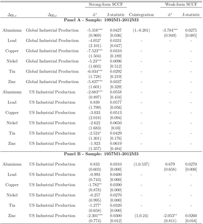
First, we analyze the pairwise behavior of metal commodity prices alone, asking whether they share common trends and/or common cycles. Results are presented in Ta-ble 1. Regarding cointegration, we find overwhelming evidence of common trends among pairwise prices (10 out of 15). Conditional on this evidence, we tested for common cycles using the GMM approach (robust to heteroskedasticity and serial correlation of unknown form), finding no signs of pairwise common cycles for the growth rates of metal-commodity prices – the only exception being the pair aluminum and lead, albeit the evidence is faint. Next, we investigate whether prices for metal commodities cointegrate and/or share common cycles with global industrial production. The analysis is pairwise, one commodity price at a time. Results are presented in Table 2 (panel A). Regarding cointegration, with the exception of aluminium, we find no evidence of a long-run relationship between metal prices and global industrial production for the last 20 years. On the other hand, results for common cycles are very different. Using the GMM approach, at 5% significance, we found evidence of strong-formcommon-cyclical features between industrial production and the following metals: copper, nickel, tin, and zinc. In addition to that, we also found evidence of weak-formcommon-cyclical features between industrial production and aluminium.

To motivate the findings of common cycles between global industrial production and the real price of copper, nickel, tin, and zinc, we detail here the results for copper, a metal for which its price is known to be associated with economic activity – the conventional wisdom of financial and business-cycle analysts for a long time7_{. In Figure 1 below, we}

plot the growth rates of copper prices – labelled ∆ln PCo

t – and the growth rates of global industrial production – labelled ∆ln IPG

t , both standardized (zero mean, unit variance).

6_{A slight caveat involves (log) aluminium prices, which rejects the null of a unit root at 5%} signif-icance when a constant is included, but rejects when a constant and trend are included. It also rejects Kwiatkowski et al. (1992) stationarity test. Thus, we chose to model it as aI(1) process.

(26)

Figure 1.1: Standardized growth rates of global industrial production and copper prices

Notice that both ∆ln PCo

t and ∆ln IPtG show signs of serial correlation, as is apparent from Figure 1 above. However, using the Ljung-Box test at 10% significance, our empirical results in Table 2 found that the following linear combination is white noise (unpredictable):

∆ln P_tCo 7.523

(1.50) ⇥∆ln IP G

t + 0.015

(0.006), (1.14)

with robust standard errors in parenthesis. This shows that ∆ln PCo

t and ∆ln IPtG are synchronized and that ln PCo

t and ln IPtG share a common cycle. As we argued in Section 2, this is consistent with a standard theory of derived demand for copper in producing industrial output for the global economy when the supply of copper is held fixed in the short run.

(27)

It is interesting to contrast the evidence of common cycles between metal-commodity prices and global industrial production with that between the former and U.S. industrial production. As is well known, there is a recent migration of industrial activity from developed countries to emerging economies, especially China and India. Global industrial production is highly influenced by the industrial production of these two countries, which may explain why it is synchronized with metal-commodity prices. On the other hand, developed countries such as the U.S. have witnessed a continued decline of its industrial sector, which may explain why we did not find strong evidence of synchronicity of U.S. industrial production and metal-commodity prices.

Quarterly Frequency

On a quarterly frequency, data for (log) prices of metals (or derived products) – Alu-minium, Copper, Lead, Nickel, Tin and Zinc – are available from 1957:01 through 2012:01. Table 3 presents results of pairwise cointegration between metal prices, reporting over-whelming evidence of cointegration between prices of different metal commodities. This is consistent with our previous finding at the monthly frequency, although our quarterly results are even stronger – 14 out of 15 pairs versus 10 out of 15.

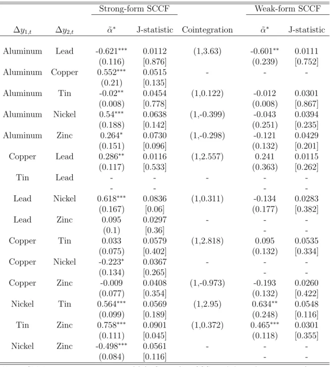
Regarding pairwise common cycles among commodity prices, we found limited evi-dence that they share common-cyclical features. Using the GMM approach described in Section 3, for all possible 15 pairwise cases, we found strong-form SCCF for 6 of them – aluminium-copper, aluminium-lead, aluminium-nickel, copper-nickel, lead-zinc, and nickel-tin. So, the growth rate of prices of aluminium and nickel are synchronized with those of other metal commodities. Similar results are also obtained for weak-form SCCF.

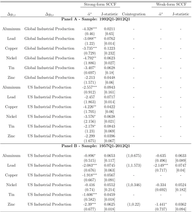
Next, using the sample 1992:1 through 2012:1, we investigate the existence of pairwise common trends and common cycles between metal-commodity prices and global and U.S. industrial production, respectively. Results are given in Table 4. First, in panel A, we find no evidence of cointegration between metal prices and global and U.S. industrial production. Second, regarding global industrial production, we find strong evidence of common cycles for aluminium, copper, and tin. For zinc, there is a common cycle at 5% significance, but not at 10%. Third, regarding U.S. industrial production, we find strong evidence of common cycles for aluminium only. For copper, tin, and zinc, there is a common cycle at 5% significance, but not at 10%. Thus, we conclude that the evidence of common cycles is stronger regarding global industrial production. This result is consistent with our findings for the monthly frequency.

(28)

evidence for lead and copper.

Annual Frequency

On an annual basis, metal-price data were provided by the United States Geological Service (USGS) from 1900 through 2010. Prices were deflated by the U.S. CPI. Table 5 presents results of pairwise cointegration between metal prices. We found overwhelming evidence of cointegration between prices of different metal commodities. Given the longer span of this annual database vis-a-vis the monthly and quarterly databases – more than twice as long – cointegrating evidence here should receive more weight vis-a-vis previous evidence. From all possible 15 cases, we found cointegration among 10 pairs of metal-commodity prices.

One interesting issue is the long-run behavior of real metal-commodity prices: while three of them displayed an obvious increase in prices (copper, nickel, and zinc) in 110 years – more than a twofold increase from 1900 to 2010 – the other three displayed an obvious decrease over time (aluminium, lead, and tin) of about 70%-90%. We conjecture here that the industrial processes of the beginning of the 20th Century used aluminium, lead, and tin in larger quantities than what was used by the end of the 20th Century. An inverse pattern being observed for copper, nickel, and zinc.

As we stressed above, cointegration analysis requires the use of long-span data. Higher frequency at the expense of span is not a substitute for the latter. Thus, our preferred results are the ones obtained in cointegration tests when using annual data, given it has the longest span – 110 years of data. Monthly and quarterly data are only available since 1957 (55 years of data) – half the span of annual data. Notice that cointegration results for annual data may not necessarily match those for monthly or quarterly data. This may be simply a consequence of the fact that the samples used in these analyses are different: 1900-2010 versus 1957-2012.

Conditional on the cointegration results, we investigate next the existence of common cycles for annual price data in pairwise analyses. Table 5 presents overwhelming evidence of common cycles for commodity prices in testing. For all possible 15 pairwise cases, we found strong-form SCCF for 14 of them, the only exception being the pair tin-zinc. Similar results are also obtained for weak-form SCCF. One point to note is that annual data for metal-prices showed much more synchronization than did quarterly and monthly data. This may be a sign that some high-frequency fluctuations that are not synchronized tend to disappear with time aggregation. Another plausible explanation for synchronization is the fact that we are using a longer sample period for the annual analysis.

(29)

to go any further on that regard8.

1.5.3 Multivariate Analysis: Cointegration and Common Cycles

for Metal Prices

We condition on previous evidence of bivariate cointegration and common cycles among metal prices and among metal prices and industrial production to build multi-variate models for (log) metal prices (or derived products) – Aluminium, Copper, Lead, Nickel, Tin and Zinc – and industrial production – either for the U.S. economy or at a global level. We expect these multivariate models to display common cycles, so we con-struct two different sets of vector autoregressive (VAR) models to serve as reduced forms: one for metal prices and global industrial production and one for metal prices and U.S. industrial production – both with seven variables – later investigating if they possess com-mon trends using Johansen’s (1991) test and comcom-mon-cyclical-feature restrictions using the GMM approach of Section 3.

We focus on monthly data, since data at the highest frequency represent best the short-run analysis which are the object of theoretical modelling of Section 2 and the empirical evidence above. We were careful in selecting the lag order of the VAR to avoid having “dynamically incomplete” models; see Vahid and Issler (2002) and Athanasopoulos et al. (2011)9_{. For monthly data and global industrial production, we selected a VAR with}

two lags in levels. There is no evidence of cointegration when all metal prices and global industrial production are jointly modelled. We selected five lags when U.S. industrial production was used instead, finding again no cointegration for the system.

Next, we present GMM tests for common-cyclical-feature restrictions in the two sys-tems described above. Results are presented in Table 6. We conclude for the existence of six cofeature vectors in both cases. Thus, all metal prices share a common cycle with industrial production (U.S. or global), given the form the contemporaneous relation-ships have in (1.6). This is consistent with our previous bivariate results, although a bit stronger, since, for the former, it was not unanimous.

To get an idea of the parsimony entailed by imposing common-cyclical-feature restric-tions in a multivarite setting, note that the unrestricted VAR in differences with one lag, such as (1.6), for six metal prices and global industrial production, has a total of 56 parameters. However, the same system where common-cyclical-feature restrictions are imposed (equation (1.9)) – with the existence of 6 cofeature vectors – has only 20 param-eters. Testing whether it is valid to impose those restrictions leads to a p-value of 0.7376,

8_{This has some implications for the implementation of the optimal forecast methods discussed above,} the main one being that we would not be able to build restricted VECMs (with common-cycle restrictions) to be later used in forecast combinations. Notice that, for the monthly frequency, we can do just that, linking theunderstanding part of this paper with theforecast part.

(30)

which validates the restricted model at usual significance levels10.

To see this explicitly, denote by ∆yt a vector stacking respectively the instantaneous growth rates of aluminium, copper, lead, nickel, tin zinc, and global industrial production, as shown in the right-hand-side of equation (1.15) below. The estimated quasi-structural

model took the form11_:

0 B B B B B B B B B B B @

∆ln PAL t

∆ln PCo t

∆ln PP l t

∆ln PN i t

∆ln PT N t

∆ln PZn t

∆ln IPG t 1 C C C C C C C C C C C A

7⇥₁

= 2 6 6 6 6 6 6 6 6 6 6 6 6 6 6 6 6 6 4

1 0 0 0 0 0 7.023 (1.13) 0 1 0 0 0 0 2.13

(1.49) 0 0 1 0 0 0 6.87

(1.50) 0 0 0 1 0 0 5.45

(1.31) 0 0 0 0 1 0 9.60

(2.06) 0 0 0 0 0 1 8.13

(1.80)

0 0 0 0 0 0 1

3 7 7 7 7 7 7 7 7 7 7 7 7 7 7 7 7 7 5 1 ⇥ (1.15) 2

4 70⇥6

0.02

(0.00) 0(0..002003) (00..002)005 (00..004002) (00..004)008 0(0..008003) (00..1404)

3

5_∆y_t ₁,

As theory and experience has taught us, the restricted VECM forecasts much better than their unrestricted counterparts. In our previous experience, to give some idea of how much better the restricted VECM forecasts, consider the following: Issler and Vahid (2001) find a 25% reduction for the determinant of the mean-squared forecast error matrix – |M SP E| – for U.S. macroeconomic aggregates, Vahid and Issler (2002) find a reduc-tion of 20% for |M SP E| when predicting U.S. coincident series using the same statistic, and Athanasopoulos et al. (2011) find a reduction of 47% for |M SP E| when predicting different measures of Brazilian Inflation.

Finally, in constructing the models that will be used in the forecast combination analysis, we will use some reduced-rank models where common cycles restrictions are imposed. Thus, our forecasts will benefit from what we have learned in the empirical analysis regarding the synchronicity of cycles in metal-commodity prices and between the former and different measures of industrial production.

1.5.4 Forecasting Metal Prices using Forecast Combinations

We now implement the forecast theory discussed in Section 3 above, where forecast accuracy is measured by the root of the mean-squared forecast error. Metal-price data used here is the same one used in the cointegration and common-cycle analyses of the

(31)

previous section, although we only focused on results for monthly and annual data alone. The former is appropriate to examine short-term forecast accuracy, whereas the latter is appropriate to measure long-term accuracy.

Our target variables in forecasting are commodity prices for Aluminium, Copper, Lead, Nickel, Tin and Zinc – made available from the London Mercantile Exchange (extracted from the IFS) for monthly frequency and from the USGS at annual frequency. For some of the estimated models, we used co-variates (predictors) which are highly correlated to metal prices. Some are related to economic activity, such as: the global industrial production, the U.S. industrial production, the Chinese industrial production, the pri-mary metals coincident index (USGS), a leading index of metals price (USGS), and some other financial-sector co-variates, such as: VIX – a volatility index, the U.S. real effective exchange rate and the S&P500 index.

Our monthly data set covers the period from January 1965 through December 2008, comprising 528 observations (T = 528). Our annual data set covers data from 1900 to 2010, comprising 111 observations (T = 111). Table 7 presents the correlations between the predictors are metal price data. Since there is evidence of a unit root for the metal prices and the co-variates used here, some series were transformed to instantaneous growth rates prior to computing correlations.

In order to fit well the cross-sectional asymptotic requirement (largeN) regarding the WLLN, we need to have a large set of diversified forecasts to eliminate the combination of idiosyncratic errors. For this reason, we chose a few classes of different econometric mod-els: AR, VAR, VECM, restricted VECM (common-cycle restrictions), all using distinct co-variates (predictors), and distinct functional forms (levels, logs), and stationarity as-sumptions (stationarity vs. difference-stationarity) for the target variable and predictors. Considering that some of these models were fairly similar, we discarded a few of those, ending up with N between 115 and 125, i.e., between 115 and 125 distinct models and distinct forecasts for each time horizon (h). Obviously, some of them are nested within each other, and we also have classes of nested models as well. As we argued before, this will not pose as long as we have a large enough number of diverse classes.

For implementing the BCAF and other combining techniques discussed above, we split the sample in three distinct parts, each with a specific purpose: the first one, from 1 toT1, to estimate the coefficients of each model; the second from T1 + 1 to T2, to compute the bias; and the third fromT2+ 1 toT, to implement truly out-of-sample forecasting, and to assess the forecast accuracy of different forecast strategies and of individual models using the root mean-squared error (RMSE) of forecasts.

To asses forecast accuracy, we constructed an algorithm which is appropriate for the bias-corrected average forecast (BCAF). For alternative forecast combinations or forecast-ing schemes, slight modifications are required. The algorithm runs as follows:

(32)

restric-tions, and a specific set of predictors), we estimate the coefficients of the regressors using the sub-sample from 1 to T1.

2. Forecast h-steps ahead the models estimated in step 1 (fh

it) from T1 to T2. Each model should be forecasted h-steps ahead T2 T1 h+ 1 times.

3. Calculate the bias associated with eachh-step ahead forecasts and each model; the bias is the average error between theh-steps ahead forecast and the observed value of the target series (from T1 to T2).

4. Forecast h-steps ahead the same models estimated in step 1 for only T2+h, using the same coefficients estimated in step 1.

5. Store the bias from step 3 and the forecast made in step 4, fh i,T2+h.

6. UpdateT1 =T1+ 1, T2 =T2+ 1.

7. Go to step 1 untilT2 =T.

8. Adjust the forecasts of each model (made fromT2+ 1 toT) by their respective bias.

9. Combine all these adjusted forecasts using equal weights.

10. Compute the RMSE of the BCAF, considering the series of metals price index as the target series.

For the monthly dataset, we took T1 = 200 and T2 = 378. Since T = 528, this leaves 150 observations to evaluate out-of-sample performance of different models. For the annual data set, we took T1 = 35 andT2 = 70. SinceT = 111, this leaves 41 observations for out-of-sample evaluation. In both cases, we kept enough data to estimate the models and two similar-size sub-samples to estimate their biases and to perform out-of-sample forecasts.

The maximum horizon was set to 6 months for monthly data and to 6 years with annual data. After computing the average bias for each forecast horizon (Bch_{), we tested} the null H0 : Bh = 0, using Issler and Lima’s t-ratio test. Tables 8 and 9 present the results, respectively with monthly and annual data.

From the results in Tables 8 and 9, we conclude that, for monthly data, none of the mean biases were significant using the t-ratio test in Issler and Lima. For annual data, zinc is the only metal for which the mean bias is clearly non-zero. There is also scattered evidence of non-zero mean bias for copper and nickel at higher horizons.

Recall from Section 4 that, when the mean bias is zero, the optimal forecast collapses to the simple average across models 1

N PN

(33)

Comparing forecast accuracy of different models

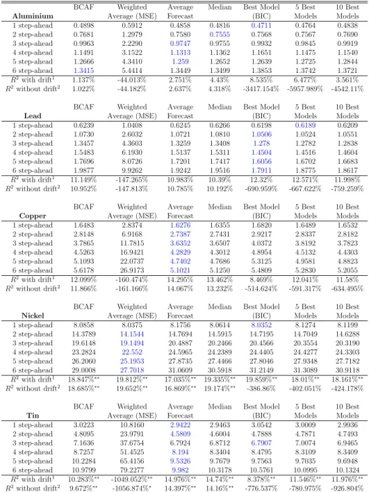
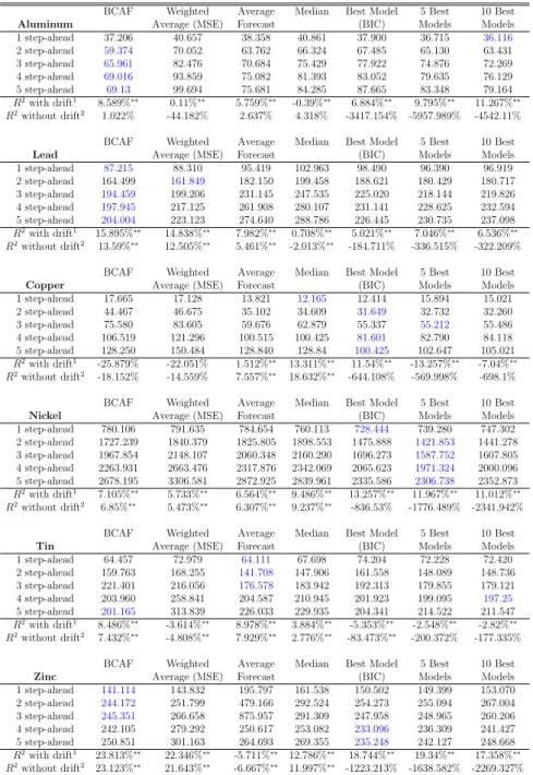
Given the theoretical results in Section 4 for optimality of combined forecasts, we con-sider here several forecast-combination strategies: (i) the bias-corrected average forecast (BCAF); (ii) the average forecast (AF); (iii) the weighted average forecast (WAF), where weights are based on the inverse of the mean-squared error for each model, normalized to add up to unity; (iv) the simple average (1/N) of the 5 best fitting models (by Bayesian Information Criteria – BIC, using a previous sample period); (v) the simple average (1/N) of the 10 best fitting models (BIC); (vi) the median forecast12_{. We computed the RMSE}

for these forecast strategies. Results are presented in Tables 10 and 11, respectively for monthly and annual data. We could not make most forecast models for zinc to converge at the monthly frequency, and thus refrain from presenting its forecast-evaluation results. For monthly data, for 1- through 6-steps ahead and across all metal prices, the best performance (by far) in terms of RMSE was achieved by the Average Forecast (AF), followed by the best model and then followed closely by the weighted average forecast (WAF). For 3 out of 5 metal prices, the Average Forecast (AF) was the best forecast strategy out of sample. This is exactly what one should expect from econometric theory (Section 4), given our evidence above that the average bias was statistically zero, i.e., that we could not reject the null H0 :Bh = 0, using Issler and Lima’s t-ratio test in Table 8. Moreover, for 4 out of 5 metal prices, forecast combinations were superior to choosing a “best” model.

In Table 10, we also present out-of-sampleR2 _{statistics (percentage) comparing} fore-cast strategies with the random-walk model with and without drift, which are important benchmarks to be beaten in the finance literature. R2_{-statistics were computed for} one-step ahead forecasts only to save space. For metal pricezt, we have:

R2 = 100_⇥

2 6 41

PT

t=T2+1 zt zbt|t 1 2

PT t=T2+1

⇣

zt zbBM K_t_|_t ₁ ⌘2

3 7 5,

wherebzt|t 1 is the one-step-ahead forecast of any given strategy andbztBM K|t 1 is the one-step-ahead forecast of the benchmark – random-walk with and without drift. For aluminium, copper and tin, our best strategy overall was the average forecast. It has R2 _{= 2}_._75% for aluminium, R2 _{= 14}_._{30% for copper, and} _R2 _{= 14}_._{98% for tin, vis-a-vis the random} walk with drift13_{. Table 10 also includes} _? _{tests for equal predictive accuracy applicable}

to nested models14_{. With the exception of nickel and tin, for all other models we cannot}

12_{For the median forecast, we have no theoretical optimality result. For the 5-best and 10-best models,} optimality can be justified as the number of best models increases with N, e.g., as a fixed quantile of models.

13_{Notice that, even when the average forecast was not the best strategy, it has beaten the random} walk.

(34)

reject the null of equal forecast accuracy between any forecast strategy and the random-walk models.

For annual data, the best forecast strategy in terms of the RMSE is to employ the bias-corrected average forecast (BCAF) – for aluminium, lead and zinc, followed by average forecast (AF) – best for tin. Thus, for 4 out of 6 metal prices, forecast combinations were the best forecast strategy out of sample; see Table 11. In terms of out-of-sample R2 _{statistics, these best models outperformed the random walk with and without drift:}

R2 _{= 8}_._{59% for aluminium,}_R2 _{= 15}_._{90% for lead,}_R2 _{= 8}_._{98% for tin, and}_R2 _{= 23}_._{8% for} zinc. Here, contrary to the evidence for monthly frequency, the best forecasts strategies are significantly different (better) than the random walk using Clark and West’s test.

Best Predictors and Models used in Forecast Combinations

Tables 12 and 13 report, respectively, the best models and predictors for monthly and annual forecasts, considering sample results across all horizons. For each out-of-sample observation, and each forecast horizon, we compared models using squared forecast errors. The model with the smallest squared error is considered the best. Tables 12 and 13 report the percentage which each model type is considered best across all horizons and out-of-sample observations. Regarding predictors, notice that the models being combined are all autoregressive, so the lags of metal prices are used as predictors in them. The category no extra predictors includes only the these lags. For some models, we use extra predictors as well, which are also reported separately.

For monthly frequency, the multivariate models – restricted vector error-correction models (VECM) described in Section 5.3 – with all metal prices and industrial production (U.S.), have the best forecasting performance overall. This connects “understanding” and “forecasting,” both in the title of this paper. Moreover, it serves as empirical validation of the theoretical model discussed in Section 2 above, where demand for metals commodities are modelled as aderived demand in producing industrial output and the supply of metal commodities are supposed to be fixed in the short run, due to the long maturity of metal-commodity projects and to their high capital intensity. The unrestricted VECMs also perform well, but not nearly as well as their restricted counterparts. Restricted and unrestricted VECMs highlight the importance of investigating short- and long-run relationships as done above.

The best predictors in monthly frequency are the lagged dependent-variables. This is expected, since most time-series models used here predict the future using the past and present. What is really informative is to look whichextra predictors do well out of sample. For monthly frequency, U.S. industrial production overwhelmingly outperforms all other predictors, with the S&P 500 and measures of realized volatility coming a far second for

(35)

different metals.

For the annual frequency, we did not did not forecast using restricted common-cycle

models (restricted VECMs), since U.S. industrial production has no serial correlation at that frequency. We were left with AR, VAR, and VECMs for forecasting metal prices. In this context, AR models were the best for aluminium and copper, VARs were best for lead and zinc, and VECMs were best for nickel and tin. For predictors, the best are lagged dependent-variables, as expected. In the class of extra predictors, U.S. industrial production and volatility measures performed well for different metals.

1.6 Conclusion and Further Research

The objective of this paper was to study (understand and forecast) spot metal price levels and changes at monthly, quarterly, and annual horizons. The data to be used consists of metal-commodity prices in a monthly and quarterly frequencies from 1957 to 2012 extracted from the IFS. At annual frequency we use USGS data from 1900 through 2010. We also employ the (relatively large) list of co-variates used in Welch and Goyal

(2008) and in Hong and Yogo (2009) , which are available for download.

Regarding the understanding part of the paper, we were able to show theoretically that there must be a positive correlation between metal-price variation and industrial-production variation if metal supply is held fixed in the short run when its demand is optimally chosen taking into account optimal production for the industrial sector. This is simply a consequence of the derived-demand model for cost-minimizing firms, which is paramount in microeconomics (Section 2). Our empirical evidence (monthly and quar-terly data) fully supports this theoretical result. Indeed, we have shown overwhelming evidence that cycles in metal prices are synchronized to those in industrial production. This evidence is stronger regarding the global economy but holds as well for the U.S. economy to a lesser degree. As far as we know, we were the first authors to investigate and find common cycles in this way, accounting for theory and empirics, and not just describing a stylized fact. This is one of the main contributions of this paper.

Essays in applied econometrics

FUNDAC

¸ ˜

AO GETULIO VARGAS

ESCOLA de P ´

OS-GRADUAC

¸ ˜

AO em

ECONOMIA

Rafael Burjack Farias Duarte

Essays in Applied Econometrics

Rafael Burjack Farias Duarte

Essays in Applied Econometrics

Tese submetida `a Escola de

P´os-Gradua¸c˜ao em Economia como

req-uisito parcial para a obten¸c˜ao do

grau de Doutor em Economia

´

Area de concentra¸c˜ao:

Econome-tria Aplicada

Orientador: Jo˜ao Victor Issler

List of Figures

List of Tables

Contents

Chapter 1

Using Common Features to

Understand the Behavior of

Metal-Commodity Prices and

Forecast them at Di

ff

erent Horizons

1.1

Introduction

1.2

Understanding the Fluctuations of Metal-Commodity

Prices

1.3

Cointegration and Common Cycles for Metal Prices

1.4

A Forecast-Combination Approach for Metal Prices

1.4.1

Forecast Combination for Nested Models

1.5

Empirical analysis

1.5.1

Data and Empirical Implementation

1.5.2

Bivariate Analysis: Cointegration and Common Cycles for

Metal Prices

1.5.3

Multivariate Analysis: Cointegration and Common Cycles

for Metal Prices

1.5.4

Forecasting Metal Prices using Forecast Combinations

1.6

Conclusion and Further Research

_ff