An econometric study on purchasing-power parity

(1)

1

Fundação Getúlio Vargas - São Paulo School of Economics

April 13

th

, 2011

Master Thesis

An Econometric Study on

Purchasing-Power Parity

Student: Flávio A. De Stéfani Machado

Supervisor: Prof. Dr. Márcio Holland de Brito

(2)

2

Fundação Getúlio Vargas – São Paulo School of Economics

April 13

th

, 2011

Master Thesis

An Econometric Study on

Purchasing-Power Parity

Student: Flávio A. De Stéfani Machado

Supervisor: Prof. Dr. Márcio Holland de Brito

Key Words & Key Topics:

1. Purchasing-Power Parity (PPP) 2. Brazil 3. Real Exchange Rate 4. Half-life

5. Economics 6. Macroeconomics 7. Econometrics 8. Time Series Econometrics

9. Unit-Root Tests 10. Cointegration 11. VAR (Vector Autoregressive)

12. VEC (Vector Error Correction) 13. Threshold Regression with Endogenous

Threshold Variable 14. Band-SETAR model 15. State Space Model

(3)

3 Machado, Flávio A. De Stéfani.

An Econometric Study On Purchasing Power Parity / Flávio A. De Stéfani Machado. - 2011.

53 f.

Orientador: Márcio Holland de Brito

Dissertação (mestrado) - Escola de Economia de São Paulo.

1. Poder aquisitivo. 2. Câmbio. 3. Econometria. 4. Análise de séries temporais. I. Brito, Márcio Holland de. II. Dissertação (mestrado) - Escola de Economia de São Paulo. III. Título.

(4)

4

Abstract

In this work we address some unresolved purchasing-power parity (PPP) puzzles;

during the process we propose a new nonlinear model and check the role of temporal

aggregation and of datasets covering only a small period of time. The hypothesis that

there is no convergence force acting on ARER has been strongly statistically rejected

and the nonlinearity showed itself as an important issue. The half-lives found for Brazil

using standard models seem to be one of the smallest ever found for a country.

However, we concluded that the speed of converge towards PPP is not a consensus yet.

Besides, we expect to give contributions to PPP literature by pointing out important

(5)

5

Resumo

Neste trabalho abordamos alguns “puzzles” da Paridade do Poder de Compra

(PPC) ainda não resolvidos; durante esse processo propomos um novo modelo

não-linear e estudamos o papel da agregação temporal e de bases de dados abrangendo

apenas um pequeno período histórico. A hipótese de que não existe uma força de

convergência agindo sobre o câmbio real ajustado (ARER) foi fortemente rejeitada

estatisticamente, e a não-linearidade se mostrou um questão importante. As meia-vidas

encontradas para o Brasil usando os modelos padrão parecem ser uma das menores já

encontradas para um país, e chegamos à conclusão de que a velocidade de convergência

em direção a PPC ainda não pode ser considerada um consenso. Pretendemos, em

adição, dar contribuições através do levantamento e esclarecimento de alguns resultados

(6)

6

Agradecimentos e Dedicatória

Agradeço ao professor Márcio Holland pela diligente orientação deste trabalho e pelos

valiosos aconselhamentos ao longo desse período de mestrado. Não posso deixar de

ressaltar que sua ajuda foi fundamental para a elaboração desta tese.

Agradeço à Fundação Getúlio Vargas e à CAPES pela oportunidade de dar continuidade

aos estudos. A FGV-EESP, em especial, forneceu um ambiente bastante propício, dando

todo o suporte necessário para realização de bons estudos e pesquisas.

Gostaria também de expressar minha gratidão aos professores que se esforçaram para

transmitir-me um pouco de seu conhecimento.

Não poderia deixar de agradecer aos amigos e colegas por todo o apoio e ajuda-mútua

durante esses anos de mestrado.

Por fim, agradeço minha mãe por ter me ajudado no período mais crítico de minha vida.

Sem essa ajuda, por consequência indireta, esta dissertação não existiria.

Dedico este trabalho:

A meu tio Sezino, in memoriam, por ter sido uma figura única, que nos proporcionou

tantos bons momentos, e contribuiu para que nossa vida fosse mais feliz e interessante.

Foi para mim um segundo pai e garanto que sua lembrança e legado não serão por nós

jamais esquecidos.

A meu avô Nilo, in memoriam, por sempre ter sido uma pessoa notavelmente bondosa e

generosa com todos que tiveram algum contato com ele, sem nunca fazer qualquer

distinção quanto à posição social ou econômica. Sem dúvida foi por essa grande virtude

(7)

7

Index of Figures and Tables

Figure 1 - Normalized Nominal Exchange Rate and Price Indexes ... 34

Figure 2 - Real Exchange Rate and Adjusted Real Exchange Rates ... 36

Table 1 - Estimated gamma Parameter, ̂ , from Model (23) ... 36

Table 2 - Quantiles for Parameter gamma in under the Null Hypothesis that = 0 (i.e., ARER Follows a Random Walk Process) ... 37

Table 3 - Residual Standard Errors Adjusted by the Degrees of Freedom ... 38

Table 4 - Half-Lives for the Real and the Adjusted Exchange Rates ... 38

Table 5 - Half-Lives for the Adjusted Exchange Rate under Model (23). ... 39

Table 6 - Half-Life Values for the ARER under Model (23). ... 39

Table A.1 - Testing the Presence of Two Unit Roots in Ln P using ADF Test ... 47

Table A.2 - Testing the Presence of One Unit Root in Ln[P] using ADF Test ... 47

Table A.3 - Testing the Presence of Two Unit Roots in Ln[P*] using ADF Test ... 48

Table A.4 - Testing the Presence of One Unit Root in Ln[P*] using ADF Test ... 48

Table A.5 - Testing the Presence of Two Unit Roots in Ln[E] using ADF Test ... 48

Table A.6 - Testing the Presence of One Unit Root in Ln[E] using ADF Test ... 49

Table A.7 - Testing the Presence of Two Unit Roots in Ln[RER] using DF-GLS Test ... 49

Table A.8 - Testing the Presence of One Unit Root in Ln[RER] using DF-GLS Test ... 49

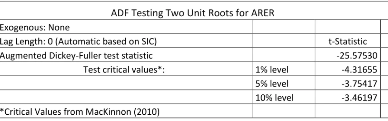
Table A.9 - Testing the Presence of Two Unit Roots in ARER using ADF Test ... 49

(9)

9

1. Introduction

Purchasing power parity (PPP) is one of the main theoretical macroeconomic

results arising from the hypothesis of rational economic agents at an environment of

open economies. PPP has always appealed to economists, one reason being that, if false,

it would put in check the hypothesis of rational agents - which is the essential

assumption of most economic theories – and/or the hypothesis of well integrated

international markets – which is a common belief nowadays.

The problem is that many studies using different methodologies were unable to

corroborate the validity of the PPP condition. Also, several studies statistically accept

PPP but find that it is only valid in the very long-run, having a large “half-life”. Why is

PPP so hard to verify? Why does it take so long for the forces behind PPP to act and

approximate the variables to the PPP condition? Those questions still entangle

economists and are still puzzles to be solved. It is timely to mention that the main PPP

puzzle nowadays is how can one conciliate the huge short-term volatility of real

exchange rates with their extremely low speed of convergence towards to PPP1. Here in

this work, we have a prior concern, namely, try to verify whether the speed of

convergence is indeed so low.

That said, it is no surprise that countless papers and studies on the issue of PPP

have emerged in recent decades. Many economists around the world are looking

forward to solving the PPP puzzles, be it by modifying the theory and/or the model, or

by using better statistical methodologies.

The main aim of this research is to address some PPP puzzles by identifying

empirically the relationship between exchange rate, domestic price and the international

price through a statistical model using monthly data, an ample historical period

(1957-2010) and a nonlinear specification; and also compare the empirical estimations made

by this model to the ones made by the most commonly used models. More particularly,

this work has several correlated objectives as following: i) present the theory underlying

the PPP (see chapter 2); ii) illustrate the cases in which the PPP standard condition is no

longer valid (see chapter 2 and 3); iii) give the intuition and/or derivation of certain

interesting and relevant results (see chapter 3); iv) present the basic statistical

1

(10)

10

procedures used to test the PPP thesis, as well their main limitations (see chapter 4); v)

show and compare some findings and proposals researchers have made (see chapters 5

and 6); vi) discuss what features a theoretic-statistical model and a econometric

methodology must have in order to be appropriate for the study of the absolute PPP (see

chapters 3 to 5); vii) and finally, by the analysis of the empirical estimations, be able to

conclude if there is enough evidences in favor of absolute PPP validity for Brazil (see

chapter 6).

It can be anticipated that the half-lives we found for Brazil using the standard

models seem to be one of the smallest half-lives ever found for a country (see Table 4),

which may indicate that the temporal aggregation and datasets covering only a small

period of time are important issues. As expected due to the small half-lives, we could

not reject absolute PPP validity applying these methodologies. Moreover, the half-lives

magnitude of one year and one or two months could mean that the low speed of

convergence puzzle is not as drastic as researchers think. Besides, we found that our

nonlinear model is at least as good as the AR(1) model in terms of adjustment level, so

it suggests that this specification might be useful for the PPP study. Also, using this

nonlinear model, we again were unable reject absolute PPP validity (see Tables 11 and

12). Furthermore, the estimated half-lives displayed at Table 6 show that the half-life

resulted from this model can be very changeful. It can be sometimes as small as ten

(11)

11

2. Basic Concepts

The Law of One Price (LOOP) is an essential and general result of economic

theory. In short, it says that, in efficient markets, the price of identical or equivalent

goods or basket of goods must be the same when expressed in terms of the same

currency. When prices diverge, a profit can be made by buying the good for the cheaper

price and selling it for the higher price until the prices converge into the same value, in

the operation known as “arbitrage”.

Economists do not expect LOOP to operate perfectly and strictly in the real world,

but most do believe that, in general, markets do not stray too far from it.

Purchasing power parity, in its turn, is just the LOOP applied to international

markets and can be algebraically depicted by:

Rt = Et / = 1 , (1)

where “R” is the real exchange rate (RER), “E” is the nominal exchange rate as defined by the foreign currency price in terms of the domestic currency , “P*” is the foreign price of any good or bundle, “P” is the domestic price of the same good or bundle, and

the subscript “t” indicates the period of time.

In order to make the equation easier to treat, it is common practice to use

logarithmic transformation to linearize the above equation, which gives2:

Ln[Rt] = Ln[Et] + Ln[ ] – Ln[Pt] = Ln[1] = 0 , using notations, we have:

rt = et + p - p = 0 , (2)

where lowercase letters indicate that the natural logarithm operator is applied to the

variable3.

2 _{L [.] is the logarith i operator.} 3

Throughout this text we are often going to refer to the natural logarithm version of the real

e ha ge rate o itti g the atural logarith term. The same is valid for other variables. In short,

ost ti es e are goi g to refer to log aria les without e tio the log ter . For i sta e, e are

(12)

12

This simply says that same goods or bundles in different countries, when expressed

in terms of the same currency, must have the same price. Therefore, if one sells a good

or a bundle of goods at any country and exchange the money received for another

country‟s currency, they would be able to buy the same good or bundle in that other

country.

Because that is a long-run relationship and every economic system has

fundamental random components – sometimes referred to as “disturbances” –, we do

not expect any of the foregoing equations to be perfectly satisfied at every point in time:

there would be always an error in the equation. This is why we require statistical tools

to check the validity of our relations. Furthermore, the real world involves quite a few

practical matters that make the observation of some idealized relations unlikely. Hence,

throughout our work we are going to try a variety of specifications for the PPP relation

and attempt to find, through statistical data analysis and economic intuition, the model

that is more compatible with reality.

Equations (1) and (2) represent the so-called “absolute PPP”. As we will show in a

while, absolute PPP as in (1) and (2) is harder to be tested and verified in practice. That

could be the reason why economists often opt to test “relative PPP” (the variational

form of absolute PPP) rather than absolute PPP, since its occurrence is more plausible.

The relative PPP condition is true whenever absolute PPP is valid, even though the

converse is not true. In other words, relative PPP is a weaker condition than absolute

PPP. The log version of relative PPP is given by:

∆rt= ∆et+ ∆pt* - ∆pt = 0 , (3)

where the operator “∆” means the first difference in time (variablet – variablet-1).

Even with rational agents and non-sticky prices, absolute PPP in its strong form as

is given in (2), is unlikely to be observed in the real world, since there are several

impediments to its occurrence. The most common obstacles are the following: freight

costs, insurance costs, customs tariffs and non-tariff barriers (E.g.: legal restrictions or

impediments). As a result, most researchers choose to test relative PPP instead, or a

modified version of absolute PPP given by:

(13)

13

The log-transformed equation is:

rt = et +p - pt = Ln[K] = k = constant , (5)

where “k” can be interpreted as transaction costs.

Unfortunately, even equations (3) and (5) may not be valid. One reason is the fact

that transaction costs are not likely to remain the same over time. Another reason lies in

the use of Price Indexes (PIs) instead of P* and P; it is not difficult to understand why

this takes place:

i) Domestic PI and foreign PI are not comparable. Since PIs are not real prices, they are

measures in relation to a basis arbitrarily chosen. Moreover, domestic PI and foreign PI

use different baskets of goods, with different weightings.

ii) One other flaw is associated with the fact that the available PIs almost always have

non-tradable goods in their compositions, and, as we know, non-tradable goods do not

abide by the LOOP.

In the next section we build several simple hypothetical situations and explain the

emerging results or problems. We expect to illustrate: i) the transaction costs

consequences; ii) how tricky can be utilizing PIs to investigate PPP; iii) other PPP

(14)

14

3. Analytical Studies

This section aims to give contributions to PPP literature by pointing out important

results and potential issues and pitfalls on PPP research. Each case illustrates a situation

where a naive and careless analysis and interpretation would fail.

Notations:

(a) The price of the domestic tradable good or bundle ( ) is

(b) The price of the domestic non-tradable good or bundle ( ) is

(c) The price of the foreign tradable good or bundle ( ) is

(d) The price of the foreign non-tradable good or bundle ( ) is

(e) α and α* are the domestic index weight for the tradable bundle and the foreign index

weight for the tradable bundle, respectively.

(f) π and π* are the domestic and the foreign inflation rate, respectively.

(g) P and P* are the domestic and the foreign Price Index, respectively.

Case 1: Is Ln[Et] = 0 + (1)Ln[Pt] + (-1)Ln[ ] realistic?

PPP condition in (2) implies Ln[Et] = Ln[Pt] – Ln[ ]. So it is intuitive to propose

a simple linear statistical regression as below and then test if 0 = 0 , 1 = 1 and 2 = -1.

Ln[Et] = 0 + 1 Ln[Pt] + 2 Ln[ ] + ut , (6)

where “ut” is the disturbance term. Or, using the notation:

et = 0 + 1 p + 2 p* + ut

But is 0 = 0 a realistic assumption? (see Cases 1 and 2). Now if we are using PIs, are

(15)

15

In general there is no reason to 1 = 1 and 2 = -1 when we are using PIs, since the

variation in “p” and “p*” might be due to the variation in the non-tradables prices. Also,

there is no reason to expect “ 1” and “ 2” to be invariant over time, once the portion of

“p” and “p*” variation due to tradable good prices variation might be varying over time.

Further, there are good reasons to “ 0”do not be the same over time, seeing that

transaction costs vary quite often. In the Appendix B, we suggest a theoretical model

that tries to describe that kind of inconstancy.

Nonetheless, later we will see that running the regression based on (6), actually, is

not an inappropriate idea, for it allows some useful corrections (farther in this text it

shall be clear).

Case 2: Impact of transaction costs.

Assumptions 2:

(a) There is just one and the same tradable good.

(b) There are freight charges equal to “τ”.

Applying LOOP, we have =1, thus Ln = Ln[1] , hence

e + p* - p + Ln[ + = 0 , then e + p* - p = -Ln[ + , therefore

e = -Ln[1+ τ] + p – p*

That is a situation where equation (5) is more reasonable than equation (2), which

is no longer valid.

Case 3: The use of PIs requires a constant in PPP equation, like in (4) and (5).

Assumptions 3:

(16)

16

(b) The PIs (P and P*) are composed of only one and the same bundle of tradable

goods.

As we know, P and P* are not the real prices of that bundle. To obtain the real

value (in monetary units) we have to multiply both indexes by some appropriate value,

let‟s say “ ” and “ *”. Applying LOOP, we have:

= 1, applying Ln[.] in both sides, we get e + p* - p = Ln[ ] , hence:

e = Ln[] + p - p*

So this is another situation where equation (5) is more reasonable than equation

(2), which is no longer valid.

Case 4: Equal inflation rates for all prices do not affect the

exchange rate of equilibrium given by (4) and (5).

We know that prices of non-tradables must not affect the exchange rate given by

PPP condition, however it generally does when using PIs. Nonetheless, we are going to

show that, under some assumptions, if the inflation rate is the same for all goods

attending the PI„s bundle, equation (4) rightly predicts that the exchange rate of

equilibrium does not change.

Assumptions 4:

(a) There is no barriers.

(b) There is a bundle, , composed of only tradable goods.

(c) There is a bundle, composed of only non-tradable goods.

(d) The foreign bundles are the same as the domestic ones.

(e) The domestic PI is P =

(17)

17

(g) α and α* belong to the interval [0,1]

(h) α ≠ α*

(i) For t ≥ 0, all prices ( evolve as the following: P0 (1+π)t, where “π”

is the inflation rate.

According to equation (4), in all periods of time the condition of equilibrium is:

Rt = Et Pt*/Pt = Et

₍ ₎

( ) ( ) = K (7)

In t = 0, equation (4) gets:

E0

₍ ₎

( ) ( ) = K , (8)

where “E0”is the exchange rate that satisfies (8).

Due to the fact that both PIs are homogeneous functions of degree 1, the inflation

does not impact on the exchange rate of equilibrium depicted in (8), thus Et = E0 for any

t ≥ 0.

Proof:

Rt = Et Pt*/Pt = Et

₍ ₎ ( ) ( ) = Et

₍ ₎

( ) ( ) =

= Et

₍ ₎

( ) ( ) = Et

₍ ₎

( ) ( ) (9)

So, in order to relation (7) keeps held, we must have Et

₍ ₎

( ) ( ) = K, but by (8)

(18)

18 Case 5: Even the same inflation rate in foreign and domestic

tradables prices may invalidate equations (4) and (5).

Assumptions 5:

(a) Assumptions 4 (a) to (h) hold.

(b) All non-tradables prices remain the same as in t = 0, except the tradables prices that

evolve by the process P0 (1+π)t in both countries.

Since prices of the tradables have the same evolution in both countries, ceteris

paribus, it is expected that the exchange rate of equilibrium determined by (4) remains

the same as in t = 0. Nevertheless, we are about to show that it does not happen when

we are using PIs.

Proof:

Rt = Et Pt*/Pt = Et

₍ ₎

( ) ( ) = K (7‟)

E0

₍ ₎

( ) ( ) = K , (8‟)

where “E0”is the exchange rate that satisfies (8‟).

Then, for t > 0, we have:

Rt = Et Pt*/Pt = Et

₍ ₎ ( ) ( ) = Et

₍ ₎ ( ) ( ) =

= Et

₍ ₎

( ) ( ) +

_.

Using (8‟)and (7‟) we have:

(19)

19

since we assumed α ≠ α*, which is a very realistic assumption.∎

(10) is a contradictory result, another distortion caused by the use of Price Indexes

(PIs).

Case 6: The acceleration of Balassa-Samuelson Effect invalidates (4) and (5).

Another drawback by using Price Indexes that include non-tradables is due to

Balassa-Samuelson Effect4. That effect is the tendency of rich countries to have higher

non-tradable prices and consequently higher Price Indexes. Thus, if one is comparing

prices between countries with substantial income level difference, he would have just a

little extra problem. It does not seem to cause extra-distortion in the estimations made

by regressions (6)since there would be just a shift at the intercept. But that can

dramatically change if the countries were experiencing considerable different

productivity growth rate in tradable sector; it would prompt different non-tradables

pricesinflation rates between the countries. In those cases it is often to mis-accept the

presence of unit root. Fortunately, it is possible to soften this distortion as we are going

to see.

Assumptions 6:

(a) Assumptions 4 (a) to (h) hold.

(b) The tradables prices remain the same as in t = 0, but the countries experience

different inflation rates in the non-tradables prices.

Since non-tradables do not abide by the LOOP, it is expected that non-tradables

prices changes do not affect the exchange rate of equilibrium determined by (4),

however it does when we are using PIs. We are about to show a case where it happens.

4

(20)

20

Proof:

Rt = Et Pt*/Pt = Et

₍ ₎

( ) ( ) = K (7‟‟)

E0

₍ ₎

( ) ( ) = K , (8‟‟)

where “E0”is the exchange rate that satisfies (8‟).

Then, for t > 0, we have:

Rt = Et Pt*/Pt = Et

₍ ₎

( ) ( ) = Et

( ) ( ) ( )

Using (8‟‟) and (7‟‟) we have:

Rt = Et

= K, what implies that Et =

≠ E0 ∎

Applying the logarithmic operator, the time trend shows up:

Ln[Et] = Ln[

] = Ln[Eo] + t (1- Ln[1+ ] - t (1- Ln[1+ ]

= Ln[Eo] + t { (1- Ln[1+ ] - (1- Ln[1+ ] } ≠ Ln[Eo] (11)

∎

There is a clear time trend in (11), so, in order to diminish the estimation bias,

we can add a time trend coefficient in the PPP regression equation or in RER unit

root tests5_.

5

(21)

21 Case 7: A case in which ₁ = 1 and ₂ = -1 in equation (6) does make sense.

Consider the estimation based on (6) using Price Indexes. We already expect to

have 0 ≠ 0 (and consequently ̂0 ≠ 0) and, by Case 0, very often 1≠ 1 and 2≠ -1 (and

consequently ̂1 ≠ 1 and ̂2 ≠ -1)6. But, if so, why it is so common in the literature to test

if 1 = 1 and 2 = -1 ?

In Case 0, we pointed out reasons to not expect 1 = 1 and 2 = -1, thus it would be

purposeless to test it, but not just that, even if we find statistically that 1 = 1 and

2 = -1, it would be mere coincidence.

However, in this section, we are going to show that, by some feasible hypotheses,

obtaining statistically 1 = 1 and 2 = -1 in the regression based on (6) using PIs is

perfectly consistent with the validity of PPP. That might be a reason of the fact that

sometimes researchers cannot reject the hypothesis of 1 = 1 and 2=-1.

Assumptions 7:

(a) Assumptions 4 (a) to (g) hold.

(b) For any arbitrary initial prices, ( , we have ( = , where

“ ” is any positive constant, and “Xt” is a random variable that determines and links the

dynamics of and .

(c) For any arbitrary initial prices, ( , we have ( = ),

where “ ” is any positive constantand “ ” is a random variable that determines and

links the dynamics of and .

(d) The true valid PPP condition is:

Ln(Et) = K0 + Ln( - Ln( = Ln( - Ln( =

= Ln( + Ln( - Ln( - n , (12)

where K0 is a positive constant that makes the adjustments in order to be valid in t = 0.

6_{Notatio : Letters ith a hat o er itself ea s the esti ate of the para eter de oted}

(22)

22

The logic behind (12) being the true valid PPP condition stems from the fact that

non-tradables - since they do not abide by the LOOP – cannot be in included in any PPP

condition.

Therefore, any model should respect the conditions below, which are derived from

(12); that is to say, any realistic model must be consistent with (12), which is by

assumption the true relation between the variables:

{ ( ) = ( ) = = = = = (13)

Now let‟s check in the regression equation (6), disregarding the error term7, what

parameters values (“ s”) are consistent with (12) and (13):

Ln(Et) = 0 + 1 Ln(Pt) + 2 Ln( =

= 0 + 1 Ln[ ( ) ] + 2 Ln[ ( ) =

= 0 + 1 n + n ( ) + n +

+ 2{ n + n + n }

From the expression above it is not hard to see what are the parameters in (6).

1 =

=

, but by (13)

= hence 1 = 1

2 =

=

, but by (13)

= - hence 2 = -1

Conclusion: If, using Geometric PIs, the non-tradables bundle price moves

proportionally to the tradables bundle price, the estimations made by the regression

based on (6) will not get distorted by the presence of non-tradables. Thus, in this case, it

would not be unrealistic to get ̂1 = 1 and ̂2 = -1 when running the regression based on

(6).

7

(23)

23 Case 8: Even with fixed non-tradable good prices, there is still distortion

in the estimations made by the regression based on (6).

Assumptions 8:

(a) Assumptions 4 (a) to (g) hold.

(b) The true valid PPP condition is:

Ln(Et) = K0 + Ln( - Ln( , (14)

where “K0”is a positive constant that makes the adjustments in order to (14) be

valid in t = 0.

Therefore, any PPP model should respect the conditions below, which are derived

from (14). That is to say, any realistic model must be consistent with (14), which is by

assumption the true relation between the variables.

{

( ) =

=

(15)

(c) For any arbitrary initial prices, ( , we have ( =

(d) For any arbitrary initial prices, ( , we have ( = )

Assumptions (c) and (d) just say that tradables bundle price varies freely while

non-tradables bundle price does not change over time. In fact, that assumption does not

appear to be much plausible. However, as we are about to see, the implications are

interesting and, due to this, we proceed on the analysis of this case.

Now let‟s check in the equation (6), disregarding the error term8, what parameters

values (“ s”) are consistent with (14) and (15):

Ln[Et] = 0 + 1 Ln[Pt] + 2 Ln[ ] =

= 0 + 1 n + n ( )

+ 2 n + n ( )

8

(24)

24

From the expression above it is not hard to see what are the parameters in (6).

1 = = = , but, by (15), ₍ ₎= , therefore:

1 = (1/ ) > 1

2 =

( ) =

=

, but, by (15), ₍ ₎= , hence:

2 = (-1/ *) < -1

Conclusion: Even if the non-tradables bundle price do not move at all, the usual

estimations made by the regression based on (6) will get distorted by the mere

presence of non-tradables. Nonetheless, if we know “ ” and “ *”- although it is

improbable -, we could correct the estimation distortion since its form is known.

By now it must be clear the hardship of working with non-tradable goods. That is

why we choose to utilize Wholesale PIs, which give less weight on non-tradables,

thereby reducing the distortions in our analysis.

In the real world, PIs are formed by hundreds of goods, including non-tradables,

and the weighting of each good varies (usually according to relative consumed

amounts). In addition, each country uses different basket of goods for its PI. However,

we expect some similarity between the chosen domestic and foreign bundle, for

(25)

25

4. Standard Methodologies

In this chapter we present the standard methodologies that researchers resort to for the purpose of studying PPP. We first present the standard single-equation linear model

methodology and after, due to some drawbacks of that methodology, we show the

standard cointegration methodology.

In an attempt to mitigate some of the distortions mentioned earlier, researchers

usually make use of the following econometric equations to test absolute and relative

PPP9, respectively:

et = 0 + 1p + 2 pt + ut (16)

∆et = 1∆p + 2∆pt +𝛆t , (17)

where “ut” and “𝛆t” are the error vectors of the regressions (16) , (17), respectively.

The residual “ût”in (16) can be interpreted as an adjusted real exchange rate (ARER).

If “ 1”and “ 2”are statistically ≠ 0, in order to find evidences of a true

relation among “e”, “p”, and “p*”10_{, we need to reject the hypothesis that}“û

t”,the

regression residual, is non-stationary, because, otherwise, the (e, p, p*) relation

could be spurious since “e”, “p” and “p*” are likely to be non-stationary11_.

In that approach, one concludes that PPP holds if “ût”is stationary in the sense that

it systematically returns to zero mean. Intuitively we would consider that PPP holds if

“ût”does not remain with high positive or negative values for long periods of time. The

economy does not usually remain stable over time, so we would not expect constant

volatility (homoscedasticity) in “ût”;rather, we would expect shocks at a variety of

levels.

The basic procedure is to test statistically if “ût”has one or more unit roots. If

rejected, “ût”is deemed stationary, and the PPP condition is accepted as valid.

9

See Wallace (2009) and Kannebley (2003).

10

1 and 2 not necessarily need to be -1 and 1, some researchers (including the authors of the

present work) accept a solute PPP e e i that ase, ut so eti es de ote it as a eaker ersio , see Kannebley (2003) and Macdonald (1993).

11

(26)

26

The foregoing is the most common methodology and is, in essence, the two-step

Engle-Granger methodology to test cointegration between three variables.

The most frequently used unit root test is ADF (Augmented Dickey-Fuller test),

which is specified as follows:

∆ût= ( - ∆ût-1 + ∑ ∆û+ t , (18)

where “ ” and“ ” are parameters to be estimated, with j = 2, 3,…d; “ t” is the error term.

If the null hypothesis, = 1, is rejected in favor of 0 < < 1, “ût” is statistically

accepted as stationary and the PPP version tested is deemed valid.

Although ADF is the most common unit root test, some researchers claim that

more suitable unit root tests exist to analyze PPP, such as the DF-GLS test. Still, it

might not be more powerful than ADF in a variety of cases12. There is no consensus so

far on which test should be used.

If we have evidence that PPP holds, the next step is to calculate its half-life, or how

long it takes to a deviation from PPP to reduce to the half its value. For example: If ût

follows an AR(1) model like ût = ût-1 + t , where “ t”is the error term, then it is

particularly easy to show that the half-life is given by13_:

Half- ife = n n (19)

The majority of the studies estimate a half-life of 3 to 5 years, which is much

longer than expected. Some studies show that the half-life of goods prices within

country is mostly months and at most usually between one and two years 14.

A possible drawback of the single-equation methodology is that it is not able to

capture the real variables dynamics, since they are analyzed separately, but are in fact

interconnected. Due to this, univariate unit-root tests, for instance, might not be the

most appropriate method to check whether a variable is stationary. Another possible

fault of the forgoing methodology is that in the Engle-Granger procedure the

cointegration relation may depend on what variable is chosen as dependent in the first

12

See Lopez, et al.(2008).

13

See Appendix A for the derivation.

14

(27)

27

step. The methodology described in this section has the advantage that it does not incur

into that shortcoming, also it treats the variables jointly, which may provide a richer

description of variables dynamics. Generally, the required multi-equation analysis is

made by using the Vector Error Correction (VEC)15 methodology, as follows.

Assuming that all variables are at most integrated of order 1, I(1), consider the

model below:

∆Xt = Γ0 + ∑Γ∆Xt-i - Π Xt-1 + t , (20)

where X = [ ], “Γ0” is a vector of constants , “Γi” with i d are matrices 3 x 3,

“d” is the maximum lag order , “ t” is the error vector.

We first determine “d” by making successive estimations of the system above and

then comparing the information criteria obtained, while also checking the normality and

the non-autocorrelation of the residuals. We then estimate system (20) using the “best”

“d”16

, obtaining estimates for remaining parameters. Next, we use the Johansen

procedure to test the rank of “Π”. If we conclude that rank(Π = 0 all variables are

I(1) but do not cointegrate, i.e., there is no long-run relationship between the three

variables, and, as such, the PPP condition is discarded. On the other hand,

rank(Π = means that no variables are integrated which is a very implausible

outcome. However, if 0 < rank(Π < the variables do cointegrate and,

consequently, there is at least one long-run relationship among them, which can be

interpreted as evidence for PPP validity. Intuitively speaking, to say that variables

cointegrate is the same as saying that a non-spurious long-run relationship holds among

them. Furthermore, in this case, the matrix“Π” can be rewritten as “ ”, where

“ ” is the “adjustment matrix” and “ ” is the cointegration matrix .

15_{See Juselius (2006).}

16_{Here, a good d e ea the d that i plies a odel that:}

i) produces a residual that has small or none autocorrelation;

ii) is one of the best by some Information Criterium, where Schwarz, Akaike and Hannan-Quinn are the most used). It is important to note that the models taken in consideration only differ by the choice of

(28)

28

The long-run relation is given by “ Xt-1”. If rank(Π = and is normalized

by = [ ] , “ Xt-1” can be interpreted as the PPP relation, i.e., the real exchange

rate adjusted by VEC methodology, which we will call “VEC-ARER”.

It is important to point out that a similar analysis can be made by including a time

trend in and/or out the cointegration relationship.

That methodology certainly has many advantages, but has some critical limitations

in its standard form. The weakness of the above procedure is that the parameters

estimations and the Johansen rank test are only valid under homoscedasticity and

(29)

29

5. Dealing with PPP Puzzles

During the last decades, many studies using different methodologies were unable

to corroborate the validity of the PPP condition. Also, several studies statistically accept

PPP but find that it is only valid in the very long-run, having a large “half-life”. Why is

PPP so hard to verify? Why does it take so long for the forces behind PPP to act and

approximate the variables to the PPP condition? Those questions still entangle

economists and are still puzzles to be solved. In this chapter, we will try to arrive in a

feasible17 methodology that is more suitable to study the PPP and those PPP puzzles.

A.M.Taylor (2001) came out with an important pitfall18 PPP studies are subject to,

temporal aggregation. Suppose the real temporal dependence of a variable is monthly,

that is, a variable in month j depends on itself in month j-1. Then, if one were to use

annual data, the simple mean of the last twelve observations, A.M.Taylor (2001) shows

that this kind of aggregation would prompt serious estimation bias. In the PPP context,

it would enlarge substantially the half-life. Of course, the larger the aggregation period,

the higher is the bias. That is one reason why we choose monthly data for our analysis.

Now we are going to present two reasonable nonlinear models, one proposed by

A.M.Taylor (2001) and other proposed by the authors of the present study.

5.1 Band-SETAR Model For The RER

A.M.Taylor (2001) points that the usage of a linear model when the correct is a

nonlinear model of the Threshold Autoregressive (TAR) kind often leads to a

considerable bias at the half-life estimation. Furthermore, A.M.Taylor (2001) uses

simulations to show that both problems combined, temporal aggregation plus

nonlinearity, generate a bias bigger than their simple sum. The nonlinearity proposed by

A.M.Taylor (2001) is given by the Band-SETAR model as below:

17

In Appendix B, we propose a model that seems to describe well the reality, though it is not feasible, in the sense that it cannot be estimated correctly.

18

(30)

30

r = {

+c + r c + r +c

r + c r +c

c + r + c + r < c

} (21)

where “rt” is the natural logarithm of real exchange rate given by equation (2); “c” and

“ ” are the parameters of the model that need to be estimated; “c” defines the

symmetric “band of inaction”; and “ ” is a “persistence parameter”, it implicitly defines the speed at which “rt” returns to its “band of inaction”, that is, how fast “rt” resumes a random walk.

If 0 < < 1, we deem the PPP condition valid (for it indicates that the RER is

stationary outside the band of inaction), and the half-life of “rt” is obtained in the usual

way:

Half-Life = Ln[1/2] / Ln[ ].

Since A.M.Taylor (2001) did not aim to focus on modeling, it did not provide an

interpretation for (21). Nonetheless, it is almost straightforward, for it is a very intuitive

model.

Following, we are going to give a possible interpretation:

(21) defines an ARER or RER interval (namely [-c ; c]) within which the agents have

no profit or utility gain in importing international goods identical (or similar) to the

domestic ones. It might be due to tariff or non-tariff barriers, disutility caused by the

delivery time, or due to any other reason you might think. As a result, within that

interval, there is no convergence force acting over the RER (or ARER), and hence the

RER moves as a random walk process. On the other hand, outside that interval, agents

get the opportunity to arbitrage, creating a force that leads the RER back to the

bandwidth [-c ; c]. Finally, it is important to notice that “ ” is constant and so the speed

(31)

31

5.2. A New Nonlinear Model Specification

Although it is a very interesting model, we suspect that the speed of adjustment

probably varies according to the equilibrium deviation. The intuitive idea is that the

larger the deviation, the bigger is the motivation for the agents to arbitrage, and

consequently, the higher the speed of adjustment. Analogously, the smaller the

deviation, the more the RER behaves similar to a white noise process. So, we propose a

nonlinear specification that allows that kind of behavior:

r = r–

(r k + , (22)

where “k” is retrieved from (5)“ ” is a parameter related to the speed of adjustment and

0 + , which implies that

0 .

To simplify, let‟s define φ≡

. It is worth to mention that “φ” has a

clear interpretation in (22), it is the percentage of correction in “t” of the disequilibrium

in “t-1”. So it is not a coincidence that when φ = 0, r = r , and when φ→ , r →k.

We can also define a variable “ ” defined as ≡

, which has an

interpretation similar to the “ ” interpretation in (21).

As it can be seen, (22) does not have the desirable “band of inaction” as (21) has;

nevertheless, when the deviation from equilibrium is small, the convergence force

implied by equation (21) is so small that can be neglected.

Some features and properties of (22):

(i) lim_→ r = k

When the deviation tends to infinity, the convergence happens in the period

immediately after the period of disequilibrium.

(ii) rt (rt-1 = k) = rt-1 = k

(32)

32

(iii) rt ( = 0) = rt-1

“rt” follows a random walk process when = 0.

Obs: That property is very convenient, since we thus can test directly the null

hypothesis that “rt” follows a random walk process.

(iv) lim_→ r = k

The convergence happens in the period immediately after the period of disequilibrium

when “ ” tends to infinity.

If k = 0 (for example if we use ARER instead of “rt”(RER)), (22) reduces to19:

rt = rt-1

+ (23)

Can be shown from (23) that20:

rt+s = , (24)

assuming there is no shocks in the considered period.

As a result, the half-life from (23) is21:

Half-Life =

; (25)

as expected, it depends on how large is the initial deviation from the equilibrium, which

is rt = 0.

Model (23) can be rewritten as a two regime model which allows asymmetry in

“ ”, as it follows:

r = {r + r 0

r + r < 0

} (26)

As it can be seen, it is just a SETAR model with a nonlinear functional form.

In this work we are going to estimate (23), adopting rt≡ ARER, and compare the

results with the estimations of the standard linear models already presented.

19

20

21

(33)

33

6. Empirical Results

The aim of this section is to present the estimations we have done and compare our

empirical findings with the ones obtained by other studies of the PPP literature.

Before that, we are going to provide the data details. The domestic price index (Pt)

used was the IPA (Wholesale Price Index, Brazil). The nominal exchange rate used is

expressed in terms of Brazilian currency per United States currency (R$/US$). Both

were retrieved from IPEA (Applied Economic Research Institute, Brazil). The foreign

price index ( ) used was the WPI (Wholesale Price Index, U.S.A.) retrieved from IFS

(International Financial Statistics from International Monetary Fund). The period for all

the three series is from January of 1957 to February of 2010, the frequency is monthly.

All the data are concerning to the end of each month.

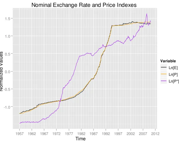
The figure below shows the normalized logarithm of P, P* and E. Clearly all the

three variables have an ascending trend. Also, it seems that the nominal exchange rate

and the domestic price index are highly correlated. However, the relationship between

the three variables is not clear by the graphic, thus we need statistical tools to unveil

(34)

34 Figure 1: Normalized Nominal Exchange Rate and Price Indexes.

Source: The series are based on data retrieved from IFS and IPEA.

Note: Here “normalized” means the following transformation for a variable, say, “y”:

y_normalized = (y – y mean) / (y standard deviation).

With the view to find the order of integration of the variables at issue, we

performed a succession of unit root tests, which are displayed at Tables A.1 to A.10.

The alternative hypothesis of the tests shown at Tables A.1, A.3, A.5, A.7 and A.9 is:

the variable has one or none unit root. The alternative hypothesis of the tests shown at

Tables A.2, A.4, A.6, A.8 and A.10 is: the variable has none unit root. Except the tests

displayed at Tables A.7 and A.8 – which are the Elliott-Rothenberg-Stock DF-GLS test

– the other unit root tests are the Augmented Dickey-Fuller test (ADF Test).

At a significance level of 5%, based on the results displayed at Tables A.1 to A.6,

we statistically accepted that “Ln[P]”, “Ln[P*]” and “Ln[E]” are I(1). As explained

earlier, that result allows us to study absolute PPP and not only relative PPP. Nominal Exchange Rate and Price Indexes

Time N o rm a li ze d V a lu e s -1.0 -0.5 0.0 0.5 1.0 1.5

1957 1962 1967 1972 1977 1982 1987 1992 1997 2002 2007 2012

Variable

Ln[E]

Ln[P]

(35)

35

As can be seen in Tables A.7 and A.8, at a significance level of 5%, “Ln[RER]”

has been statistically accepted as having one unit root, what means “Ln[RER]” is non -stationary and consequently absolute PPP is not deemed as valid using the

corresponding methodology.

As shown in Tables A.9 and A.10, using the critical values formula suggested by

MacKinnon (2010), we reject, at a confidence level of 5%, that the adjusted real

exchange rate (ARER) has one or more unit roots. The fact that ARER was statistically

accepted as stationary by the corresponding methodology constitutes an evidence for the

validity of absolute PPP.

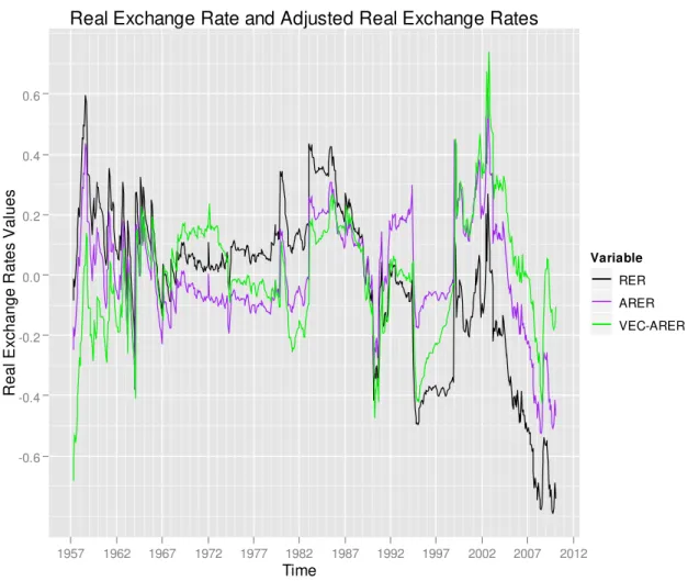
Figure 2 shows together the graphics of RER22, ARER and VEC-ARER. Although

the general behavior is similar for all variables, at some periods of time the behaviors

diverge considerably, it suggests that the real exchange rate is sensitive to the

methodology adopted to calculate it.

22_{Re e} _{er that al ost e er ti e e e tio RER e are a tuall referri g to the}

(36)

36 Figure 2: Real Exchange Rate and Adjusted Real Exchange Rates.

Source: The series are based on data retrieved from IFS and IPEA.

The next table presents the estimated value of the parameter “ ” from (23) by the

nonlinear least squares method.

Table 1: Estimated “gamma” Parameter,“ ̂”, from Model (23).

Model / Parameter Estimated Gamma Coefficient

ARER in (23) 0.16730

In order to check the statistical significance of “ ” in (23) we estimated the

quantiles under the hypothesis that = 0 (i.e., ARER follows a random walk process).

We obtained those estimates through two different methods: the first is the

Real Exchange Rate and Adjusted Real Exchange Rates

Time R e a l E xch a n g e R a te s V a lu e s -0.6 -0.4 -0.2 0.0 0.2 0.4 0.6

1957 1962 1967 1972 1977 1982 1987 1992 1997 2002 2007 2012

Variable

RER

ARER

(37)

37

parametric bootstrap method, the second is the method of Monte Carlo simulation using

gaussian error terms with the same mean and standard deviation as the residual. The

results are at Table 2.

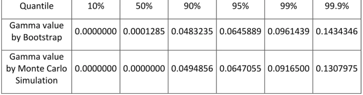
Table 2: Quantiles for Parameter “gamma” in (23) under the Null Hypothesis that = 0 (i.e., ARER Follows a Random Walk Process).

Quantile 10% 50% 90% 95% 99% 99.9%

Gamma value

by Bootstrap 0.0000000 0.0001285 0.0483235 0.0645889 0.0961439 0.1434346 Gamma value

by Monte Carlo Simulation

0.0000000 0.0000000 0.0494856 0.0647055 0.0916500 0.1307975

Since ̂ = 0.16730, we were able to reject the null hypothesis that ARER follows a

random walk process at a significance level smaller than 0.1%, what means a strong

evidence in favor of the existence of a convergence force over ARER.

Although during the last two decades there has been more evidences supporting

PPP as exposed in Rogoff (1996), Froot & Rogoff (1995), M.P.Taylor (2003), there are

still some papers as Murray & Pappel (2005), Cuddington & Liang (2000) and Zini &

Cati (1993) with contrary evidence. However, this study, as shown at Tables 2, A.9 and

A.10, provides one more evidence of PPP validity.

One of the criteria to decide whether a model is better than other concurrent

models is to check if its adequacy with the data is the highest. With that in mind, we

compared in Table 3 the residual standard errors23 of (23) and an AR(1) model, both

taking ARER as the dependent variable.

23

(38)

38 Table 3: Residual Standard Errors Adjusted by the Degrees of Freedom.

Regression / Parameter Residual Standard Error AR(1) for ARER 0.05521 on 636 degrees of freedom

(23) for ARER 0.05511 on 636 degrees of freedom

Bearing in mind that the two regressions above have the same dependent variable

and the same number of parameters, we can say that our nonlinear model is at least as

good as the linear model (autoregressive of order 1) in terms of adjustment level, as we

can see by their residual standard errors. This might mean that nonlinearity is an

important issue on PPP study.

The main method we used to estimate the half-lives for the real exchange rate and

the other adjusted real exchange rates, ARER and VEC-ARER, consists in finding the

ARIMA model that is the best according to the Schwarz information criterium, and then

applying the formula given by equation (19) if the chosen model is an AR(1). Where the

chosen model is not an AR(.) of any order, there is no trivial and general half-life

calculation method, therefore requiring specific analysis. Note that, when (23) is applied

for ARER, the half-life is analytically given by (25). However, as expression (25)

makes it clear, the half-life depends on the initial deviation from equilibrium.

The “best” ARIMA model for the real exchange rates – RER, ARER and

VEC-ARER – according to all of the information criteria considered24 was a simple AR(1), so

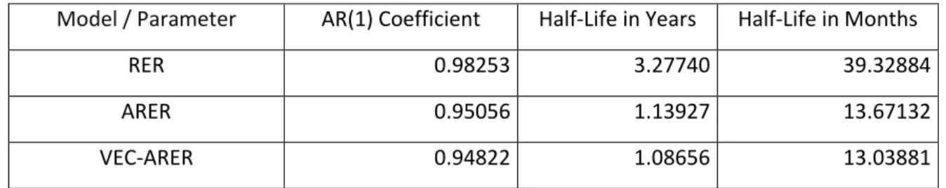
the half-lives could be easily calculated. The results are presented in Table 4.

Table 4: Half-Lives for the Real and the Adjusted Exchange Rates.

Model / Parameter AR(1) Coefficient Half-Life in Years Half-Life in Months

RER 0.98253 3.27740 39.32884

ARER 0.95056 1.13927 13.67132

VEC-ARER 0.94822 1.08656 13.03881

24

(39)

39

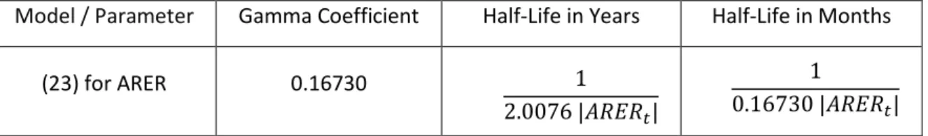
In the table below, it is shown the estimated half-life formula from model (23) for

the ARER.

Table 5: Half-Lives for the Adjusted Exchange Rate under Model (23).

Model / Parameter Gamma Coefficient Half-Life in Years Half-Life in Months (23) for ARER 0.16730

In the next table, we calculate some values for the half-lives of the Table 5. In

order to get some idea of the half-lives for the observed ARER serie, we replace the

“|ARERt|” of Table 5 by the median of |ARER| serie and its maximum value.

Table 6: Half-Life Values for the ARER under Model (23).

Frankel & Rose (1996), Pappel (1997), M.P.Taylor (2003), M.P.Taylor (1996),

Abuaf & Jorion (1990), Froot & Rogoff (1995), Rogoff (1996), altogether these papers

seem to provide a consensus that the half-lives are of the order of two and half to six

years. Nevertheless, the ARER half-lives estimates we present in Table 4 contradict that

consensus, what may suggest that the amplitude and the frequency of the data

substantially affect the estimations results or that there is some unusual heterogeneity at

the mean-reversion process of the ARER between Brazil and U.S.A.25. However, the

economic relationship between those two countries does not seem to be so peculiar to

justify the hypothesis of heterogeneity. Unfortunately, there is almost none papers

providing half-life estimates for Brazil, so that we could not make comparisons.

Regarding model (23), since the shocks that prompt the deviations from equilibrium are

very changeful, the half-life resulted from this model is also very changeful. It can be

25

See Koedijk, et al. (2011) for more details about the heterogeneity issue.

(40)

40

sometimes as small as ten months and sometimes as high as the magnitudes usually

found in PPP literature, as can be viewed in Table 6. In terms of adjustment level,

model (23) is as good as an AR(1) to explain the ARER behavior, therefore the real

magnitude of the speed of convergence is still uncertain and actually far from a

(41)

41

7. Conclusions

For decades economists has been entangled by PPP puzzles and there are still

many doubts on the issue. In the present research we opted to deal with and study more

accurately two of them, namely, the difficulty to statistically accept the PPP condition,

and the unexpected long time the RER, or the ARER, takes to return back to the

equilibrium value preconized by the absolute PPP. We intended with the present work

to check, if one applies more suitable methodologies for the study of the absolute PPP,

whether the mentioned puzzles are still puzzles. In this regard, we: i) propose an

original nonlinear model, check its suitability for Brazilian monthly data, and analyze

the estimation results; ii) make new estimations for some of the most commonly used

PPP models using (Brazilian) monthly data in order to mitigate the temporal

aggregation problem and increase the number of observations, thereby exploiting a

larger amount of information; moreover, we use a wide period of observation in order to

be able to get the long-run behavior of the variables concerning to PPP.

This work also tried to give contributions by pointing out some results and

problems inherent to PPP study that, if ignored, lead to non-negligible methodology

errors.

The ARER half-lives we obtained for Brazil using standard models seem to be one

of the smallest half-lives ever found for a country (see Table 4), which may indicate that

the temporal aggregation and datasets covering only a small period of time are

important issues. As expected due to the small half-lives, we could not reject absolute

PPP validity applying these methodologies. Moreover, the half-lives magnitude of one

year and one month could mean that the puzzles at issue are not as drastic as researchers

think.

Besides, we found that our nonlinear model is at least as good as the linear model

(autoregressive of order 1) in terms of adjustment level, so it suggests that this

specification might be useful for the PPP study. Using this nonlinear model, we again

were unable reject absolute PPP validity (see Tables 11 and 12). Furthermore, the

estimated half-lives displayed at Table 6 show that the half-life resulted from this model

(42)

42

high as the magnitudes usually found in PPP literature (2.5 to 6 years). With that result,

since we do not know yet for sure the specification that better depicts the reality (see

Table 3), we conclude that the magnitude of the convergence speed towards PPP is

actually far from a consensus. Nonetheless, our estimations reached one consensus, the

hypothesis that there is no convergence force acting on ARER has been strongly

rejected, what constitutes an evidence in favor of the absolute PPP validity26.

In this work we only use Brazilian data, so we plan in the near future to test if

those findings are valid for other countries too. By analyzing data of other countries, we

hope to get enough information to decide which model better depicts the reality: the

nonlinear model presented here or the standard models.

26

(43)

43

Appendix A: Some Derivations

Deriving (23) from (22) in case of k = 0:

r = r–

(r k + ⇒ r = r –

(r + ⇒

⇒ r = r

+ = r

+ = r + ∎

Deriving (24) from (23):

rt = rt-1

⇒ rt+1 = ⇒

⇒ rt+2 = rt+1

= [ ] = [ ] = ⇒

⇒ rt+3 = rt+2

= [ ] = [ ] =

⇒ … By now it must not be hard to see the pattern that has emerged from the

recursion: rt+s = , (24)

for any “t” that belongs to integer set and for any “s” that belongs to natural numbers.

To prove this result, we are going to use the mathematical induction method, as

follows:

Assuming as valid for s = j let’s check if remains valid for s = j+ .

So, we have that rt+j = , what implies that rt+j+1 =

.

Since r =

by the model equation (23), rt+j+1 =

| | |

. Since 0 ,

rt+j+1 =

| |

_{| |} ⇒ ⇒ rt+j+1 = .

Hence, if (24) is valid for s = j, (24) is also valid for s = j+1.

We know, by (23), that (24) is valid for s = 0. As a result, (24) is valid for s = 1, 2,

…

(44)

44 Deriving (25) from (24):

rt+s = ⇒ rt+H = = ⇒ + r = 2 ⇒

⇒ alf-Life =

∎

Deriving (19):

Consider the AR(1) model ̂t = ̂t-1 + t . In addition we have to assume “ t”, the

disturbance term, is equal to zero for all t, i.e., there are no shocks. Then, ̂s = ̂0.

Applying the Half-Life (H) definition, we have:

(45)

45

Appendix B: Time-Varying Parameters Model

A notable shortcoming in the standard methodology is the assumption of

constant parameters in equation (6), which is poorly plausible in the real world.

However, the usual estimation technology, i.e. ordinary least squares, cannot

handle shifting parameters. It requires the use of the so-called article Filter

estimation technique. But let’s first present the model we propose in its state space form:

{

= Exp[ ]p + Exp[ ]p + 0

= + 0

= + 0 }

(27)

Note that we cannot apply the standard “Kalman Filter” estimation technique

since the model contains nonlinearities.

The model is intuitively simple. All parameters follow a random walk, i.e., they tend to keep the same unless affected by a shock, which is permanent. The exponential

function is applied to the parameters in order to impose them to be positive; however,

although Exp[ 1,t ] and Exp[ 2,t ], by construction, are not random walks and have

an asymmetric probability distribution, they exhibit an inertia similar to a random

walk process. This kind of inertia has an intuitive appeal, and it is no surprise that, in

the real world, several variables indeed behave statistically as random walks.

The advantage of that model is its attempt to get the parameters dynamics and

thereby make the model more realistic.

Although we think the model above is a reasonable approximation of the reality, it

is very problematic to test empirically if it is indeed a “good” model27

, since the

estimation technique, in this case, artificially produces an extremely high match with

the data, no matter what the true data generation process is28. In addition, (27) has too

much randomness. In order to turn (27) into an useful model, it would require much

27 _{good odel here ea s a odel that}

explains well the reality.

28

(46)

46

extra information, thereby knowing more about the behavior of “ ” , “ ” and

“ ”.

For those reasons, we decided not to perform estimations for this model, and let it

(47)

47

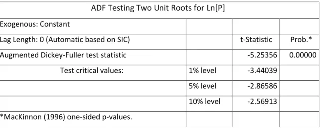
Appendix C: Tables

Table A.1: Testing the Presence of Two Unit Roots in “Ln(P)” using ADF Test.

ADF Testing Two Unit Roots for Ln[P]

Exogenous: Constant

Lag Length: 0 (Automatic based on SIC) t-Statistic Prob.* Augmented Dickey-Fuller test statistic -5.25356 0.00000

Test critical values: 1% level -3.44039

5% level -2.86586

10% level -2.56913

*MacKinnon (1996) one-sided p-values.

Table A.2: Testing the Presence of One Unit Root in “Ln[P]” using ADF Test.

ADF Testing One Unit Root for Ln[P]

Exogenous: Constant, Linear Trend

5% level -3.41688

10% level -3.13080

(48)

48 Table A.3: Testing the Presence of Two Unit Roots in “Ln[P*]” using ADF Test.

ADF Testing Two Unit Roots for Ln[P*]

5% level -3.41691

10% level -3.13082

Table A.4: Testing the Presence of One Unit Root in “Ln[P*]” using ADF Test.

ADF Testing One Unit Root for Ln[P*]

5% level -3.41691

10% level -3.13082

Table A.5: Testing the Presence of Two Unit Roots in “Ln[E]” using ADF Test.

ADF Testing Two Unit Roots for Ln[E]

Exogenous: None

5% level -1.94132

10% level -1.61637

An econometric study on purchasing-power parity

Fundação Getúlio Vargas - São Paulo School of Economics

April 13

, 2011

Master Thesis

An Econometric Study on

Purchasing-Power Parity

Fundação Getúlio Vargas – São Paulo School of Economics

April 13

, 2011

Master Thesis

An Econometric Study on

Purchasing-Power Parity

Abstract

Resumo

Agradecimentos e Dedicatória

Table of Contents

Index of Figures and Tables

1. Introduction

2. Basic Concepts

3. Analytical Studies

4. Standard Methodologies

5. Dealing with PPP Puzzles

5.1 Band-SETAR Model For The RER

5.2. A New Nonlinear Model Specification

6. Empirical Results

7. Conclusions

Appendix A: Some Derivations

Appendix B: Time-Varying Parameters Model

Appendix C: Tables