❊♥s❛✐♦s ❊❝♦♥ô♠✐❝♦s
❊s❝♦❧❛ ❞❡
Pós✲●r❛❞✉❛çã♦
❡♠ ❊❝♦♥♦♠✐❛
❞❛ ❋✉♥❞❛çã♦
●❡t✉❧✐♦ ❱❛r❣❛s
◆◦ ✻✾✷ ■❙❙◆ ✵✶✵✹✲✽✾✶✵
❈❛♥ ❛ ❍❛❜✐t ❋♦r♠❛t✐♦♥ ▼♦❞❡❧ r❡❛❧❧② ❡①♣❧❛✐♥
t❤❡ ❢♦r✇❛r❞ ♣r❡♠✐✉♠ ❛♥♦♠❛❧②❄
❈❛r❧♦s ❊✉❣ê♥✐♦ ❞❛ ❈♦st❛✱ ❏✐✈❛❣♦ ❳✳ ❱❛s❝♦♥❝❡❧♦s
❖s ❛rt✐❣♦s ♣✉❜❧✐❝❛❞♦s sã♦ ❞❡ ✐♥t❡✐r❛ r❡s♣♦♥s❛❜✐❧✐❞❛❞❡ ❞❡ s❡✉s ❛✉t♦r❡s✳ ❆s
♦♣✐♥✐õ❡s ♥❡❧❡s ❡♠✐t✐❞❛s ♥ã♦ ❡①♣r✐♠❡♠✱ ♥❡❝❡ss❛r✐❛♠❡♥t❡✱ ♦ ♣♦♥t♦ ❞❡ ✈✐st❛ ❞❛
❋✉♥❞❛çã♦ ●❡t✉❧✐♦ ❱❛r❣❛s✳
❊❙❈❖▲❆ ❉❊ PÓ❙✲●❘❆❉❯❆➬➹❖ ❊▼ ❊❈❖◆❖▼■❆ ❉✐r❡t♦r ●❡r❛❧✿ ❘❡♥❛t♦ ❋r❛❣❡❧❧✐ ❈❛r❞♦s♦
❉✐r❡t♦r ❞❡ ❊♥s✐♥♦✿ ▲✉✐s ❍❡♥r✐q✉❡ ❇❡rt♦❧✐♥♦ ❇r❛✐❞♦ ❉✐r❡t♦r ❞❡ P❡sq✉✐s❛✿ ❏♦ã♦ ❱✐❝t♦r ■ss❧❡r
❉✐r❡t♦r ❞❡ P✉❜❧✐❝❛çõ❡s ❈✐❡♥tí✜❝❛s✿ ❘✐❝❛r❞♦ ❞❡ ❖❧✐✈❡✐r❛ ❈❛✈❛❧❝❛♥t✐
❊✉❣ê♥✐♦ ❞❛ ❈♦st❛✱ ❈❛r❧♦s
❈❛♥ ❛ ❍❛❜✐t ❋♦r♠❛t✐♦♥ ▼♦❞❡❧ r❡❛❧❧② ❡①♣❧❛✐♥ t❤❡ ❢♦r✇❛r❞ ♣r❡♠✐✉♠ ❛♥♦♠❛❧②❄✴ ❈❛r❧♦s ❊✉❣ê♥✐♦ ❞❛ ❈♦st❛✱ ❏✐✈❛❣♦ ❳✳ ❱❛s❝♦♥❝❡❧♦s ✕ ❘✐♦ ❞❡ ❏❛♥❡✐r♦ ✿ ❋●❱✱❊P●❊✱ ✷✵✶✵
✭❊♥s❛✐♦s ❊❝♦♥ô♠✐❝♦s❀ ✻✾✷✮
■♥❝❧✉✐ ❜✐❜❧✐♦❣r❛❢✐❛✳
Can a Habit Formation Model
really explain the Forward
Premium Anomaly?
∗
Carlos E. da Costa
Funda¸c˜ao Getulio Vargas
Jivago X. Vasconcelos
Funda¸c˜ao Getulio Vargas
May 11, 2009 - 11:43 am
Abstract
Verdelhan(2009) shows that if one is to explain the foreign exchange forward premium behavior usingCampbell and Cochrane (1999)’s habit formation model one must specify it in such a way to generate pro-cyclical short term risk free rates. At the calibration procedure, we show that this is only possible in Campbell and Cochrane’s framework under implausible parameters specifications given that the price-consumption ratio diverges in almost all parameters sets. We, then, adopt Verdelhan’s shortcut of fixing the sensivity functionλ(st) at its steady state level to
attain a finite value for the price-consumption ratio and release it in the simulation stage to ensure pro-cyclical risk free rates. Beyond the potential inconsistencies that such procedure may generate, as suggested by Wachter (2006), with pro-cyclical risk free rates the model generates a downward sloped real yield curve, which is at odds with the data. Keywords: Forward Premium Puzzle, Equity Premium Puzzle, Habit formation, Asset Pricing; J.E.L. codes: G12, G15.
Introduction
The forward premium anomaly or Forward Premium Puzzle – FPP, henceforth - is closely related to the failure of Uncovered Interest Parity – UIP henceforth – relation, i.e. if covered interest parity holds then the forward discount and the interest differ-ential should be unbiased predictors of the ex-post change in the spot rate, assuming rational expectations. The UIP arises from a simple arbitrage argument in a risk neutral world. Higher interest rates imply currency devaluation so that the expected returns on domestic and foreign short-term bonds are equalized. Once we depart from risk neutrality, violations of UIP need not be puzzling, it is always possible to define a risk premium that accommodates the behavior of excess returns on foreign markets.
∗ We thank Caio Almeida, Jo˜ao Ayres, Jefferson Bertolai, Luis Braido, Jaime de Jesus Filho and
The relevant questions are whether this risk premium is derived from a sensible model and whether it is compatible with the behavior of other asset prices. The main difficulty one faces in trying to accommodate foreign market facts with a risk model is the poor performance of most asset pricing models, as evidenced by the Equity Premium Puzzle—EPP.
It is in this context that the results in Verdelhan (2009) seem very heartening. There it is shown that the external habit model of Campbell and Cochrane (1999) may, at the same time, account for most stylized facts in both domestic and foreign markets.
Campbell and Cochrane(1999) external habit formation model delivers time-varying countercyclical risk premia. In bad times investor’s risk aversion is higher, so he de-mands a larger risk premium. Hence, when consumption falls, expected returns, return volatility and the price of risk rise. Economic fluctuations generate in the model impor-tant aspects of asset prices behavior: (a) long-horizon predictability of excess returns from consumption-price ratio; (b) mean reversion in returns; (c) high stock price and return volatility despite smooth consumption growth. All these characteristics make the model a suitable candidate for the exercise conducted by Verdelhan(2009).
In this paper, we follow Verdelhan’s lead and calibrate Campbell and Cochrane
(1999) model for US post-war data and created endowment processes for fictitious countries based on US data. The process of each fictitious country is generated arbi-trarily aiming to reach a target correlation with US consumption data. Thus, we can use the same model to generate the stochastic discount factor for each fictitious coun-try, which allow us to evaluate the real exchange rate between US and its counterparts. So, we are able to evaluate an appropriate forward premia in currency markets which fits domestic markets asset behavior.
simultaneously.
As we will show, this assumption has a significant impact on real yields. In contrast with empirical data, which usually exhibits an upward sloping real yield curve, we show that when risk free rates are pro-cyclical the habit formation model delivers a downward sloping real yield curve. This behavior is at odds with evidence in almost all data sets. In a broad sense, although our results seem to indicate that the original Campbell and Cochrane consumption-based model is not able to produce the behavior of exchange markets we cannot state it for sure, given the inconsistency in the procedure. Indeed, this another drawback of this application of the model: the calibration shortcut used to reach a finite price-consumption ratio and all its potential inconsistencies. These potential inconsistencies should result given that stock market returns depend on price-consumption ratio.
The remainder of the paper is organized as follows. Section 2 explains the FPP puzzle and presents UIP null hypothesis in nominal and real terms. Section 3 describes the model and how the exchange rates are attained. Moreover, is derived a sufficient and necessary condition to reproduce the FPP evidence in simulated data. Section 4 exhibits the methodology and simulation results after having imposed a constant sensi-bility function, besides a critical analysis about that assumption. Section 5 concludes.
1
Literary Review: a glance at the FPP
1.1 The null hypothesis in nominal terms
Following the seminal work of Hodrick (1987), a large volume of research aiming at evaluating the efficiency of forward markets for foreign exchange has been produced. The focus of such agenda has been to explain the most puzzling aspect of this market’s behavior: an apparent large conditional bias in the use of forward rates to forecast the future spot exchange rates.
If a market is said to be efficient, in equilibrium, all agents have access to all relevant information in the market and possibilities of excesses of returns by arbitrage are impossible.1
In an efficient market with rational expectations and that risk neutrality by the agents, the expected earnings in keeping a foreign currency more valued than the domestic will be compensated by the opportunity cost of maintaining foreign assets instead domestic assets.
The following expression,
1 +it= (1 +i
∗
t)
EtEt+1
Et
, (1)
for UIP holds, whereitis the domestic nominal interest rate;i∗t is the equivalent foreign
nominal interest rate,Et andEtEt+1 are, respectively, the spot exchange rate at time t and the expected future spot exchange rate evaluated in units of domestic currency. In all that follows,Etrepresents the mathematical expectation conditional on information
available to the market at timet.
Thus, in logs, and if expectations are rational, et+1−et=Et(et+1−et) +ǫt+1 with
ǫt+1 uncorrelated with timet variables representing the error on future spot exchange rate expectations. Using log-approximation log(1 +x)∼x, the expression (1) becomes
Et(et+1−et) =Et∆et+1=it−i∗t (2)
with et = log(Et). Using the covered interest parity relation in logs ft = it−i∗ t +et,
whereftrepresents the log of exchange rate one period forward, the expression (2) can
be rewritten as the forward discount version of UIP
Et∆et+1=α+β(ft−et) +εt+1 (3)
This regression appears frequently in the literature. Generally, the null hypothesis tested isα = 0 andβ = 1 assuming thatEt[εt+1|Ωt] = 0 andEt[εt+1(ft−et)|Ωt] = 0
where Ωt is the available information set in period t. Under this null hypothesis, ft is
an unbiasedness predictor of spot exchange rate one period forward.
However, empirical studies likeHansen and Hodrick(1980) and many others,2 have produced strong evidence against the unbiasedness hypothesis showing an apparent large conditional bias in models which use forward rates to forecast the future spot exchange rates. A large volume of studies have found that currency devaluation are negatively correlated with the cross-country interest differentials, i.e. currencies with higher interest rates tend to appreciate. This outcome is often referred to as the forward discount anomaly. Indeed, according to Froot(1990), the mean estimate ofβ
over 75 empirical works is −0.88, challenging on empirical grounds the unbiasedness hypothesis.
Because this widespread evidence poses a serious challenge to our understanding of international financial markets, the nature of this anomaly has been the focus of an
2
enormous literature concerning the efficiency of these markets. We can mention three main lines of work aiming at explaining the FPP. First, the existence of a distortion on the component of rational expectations carried by exchange market participants turns the forward discount anomaly a rejection of the rational expectation hypothesis. Second, market imperfections as source of asymmetries in foreign exchange markets, which are supported by evidence of conditional-mean nonlinearities in risk premia. Third, the presence of a risk premium not appraised in the UIP expression.
Concerning the first research line, one can mention as example Rogoff (1979) who suggested that, in a context where agents attribute a low probability for rare nature states (for instance, great changes in economy foundations) an asymmetry will ap-pear in a prior event distribution, the well-known Peso Problem. Froot and Frankel
(1989) attributed the anomaly to expectation errors. In a recent work, Bacchetta and Van Wincoop (2006) developed a model of rational inattention that produces sticky prices and it is consistent with the FPP. The role of market imperfections in FPP explanation, as the second research line, could be seen, for instance, in Coakley and Fuertes (2001) where authors considered an extension of the Dornbusch exchange rate overshooting theory as a special case of asymmetric or nonlinear behavior in foreign exchange markets that fits the FPP.
The third line of research, perhaps the most natural explanation for why the forward premium predicts the wrong direction of exchange rate movements, focuses on a wedge between expected changes and actual changes driven by a risk premium. How to model the risk premium is the challenge of this literature and the purpose of our work. Hodrick
(1987) concluded: ”We do not yet have a model of expected returns that fits the data” (p.157). Engel(1996) provides a survey.
Many researchers tried to reproduce models of asset pricing that taking into ac-count the forward premium correctly in the cross-ac-country exchange market. Those models reproduced a negative slope coefficient when the theoretical spot rate changes are regressed on the theoretical lagged forward premium. See e.g. Backus et al.(1995),
Bekaert (1996), Bekaert et al. (1997) and Macklem (1991). Unfortunately, many of these models cannot explain most of already mentioned foreign exchange market styl-ized facts.
US government bonds,3 individuals must have implausible high risk aversion according
to classical models. In fact, the consumption-based asset pricing model (CCAPM) with power utility fails to explain important facts about stock returns, including the high equity premium, the high volatility of returns and the countercyclical variation in the equity premium.4
However, consumption-based models have been resurrected for forward risk premia evaluations by appealing to more sophisticated preferences. Moore and Roche(2007) relies upon external habit preferences imbedding them into a monetary model. More recently,Verdelhan(2009) has also forwarded a model using external habit preferences, which led to quantitatively large risk premia and matched the variance of real exchange rates. The purpose of our work is very similar to the forthcoming work by Verdelhan. Contrary to him, our findings are not favorable to the model.
1.2 The null hypothesis in real terms
The condition for the absence of profit opportunities by a risk neutral domestic investor endowed with rational expectations from forward market speculation is
Et
Ft− Et+1
Pt+1
= 0,
wherePt+1 is the domestic price of goods.
For simplicity, assume that all variables above are conditionally log-normally dis-tributed.5 We may, in this case, rewrite the expression above as
Et(et+1) =ft−0.5V art(et+1) +Covt(et+1, pt+1).
Note that the risk premium rpt=ft−Et(et+1) for the risk neutral investor is not
zero because the term 0.5V art(et+1)−Covt(et+1, pt+1) is not zero. This term is the
Jensen inequality term—JIT.6 Thus,f
tis not necessarily a conditional predictor ofet+1
despite the very small absolute value of JIT. According toEngel(1996), most empirical works do not consider the JIT due to its very small size.
3This feature prevails in many other industrialized countries, as pointed out byKocherlakota(1996). 4
SeeGrossman and Shiller(1981),Shiller(1981) andKandel and Stambaugh(1990). For a deeper discussion about EPP, seeKocherlakota(1996) andMehra and Prescott(2003). Both reviews present a detailed analysis of these explanations in financial markets and conclude that the puzzle is real and remains unexplained. Subsequent reviews of the literature have similarly found no agreed upon resolution.
5
An analytically convenient assumption, very common in finance literature, though not very suc-cessful on empirical grounds.
6
The true risk premium can, nonetheless, be calculated as follows
trpt≡ft−Et(et+1)−0.5V art(et+1) +Covt(et+1, pt+1) =rpt−JIT.
By the same token, a foreign risk neutral investor would require a risk premium given by
trpt=ft−Et(et+1)−0.5V art(et+1) +Covt(et+1, p∗t+1+et+1),
wherep∗
t+1is the log of the foreign price in foreign currency. The two expressions above will be the same when the purchasing power parity—PPP—condition holds, i.e.,
pt+1 =p∗t+1+et+1.
If PPP does not hold, then domestic and foreign investors evaluate real returns differently, so that there would be no equilibrium with risk neutral investors in each country.
The null hypothesis described in the latter subsection is equivalent to
rpt=ft−Et(et+1) = 0.
Considering the covered interest parity again and risk neutrality of domestic investor we can rewrite the null hypothesis as
it−i
∗
t =Et(et+1−et) + 0.5V art(et+1)−Covt(et+1, pt+1). (4)
When a foreign investor is assumed to be risk neutral, the null is
it−i∗t =Et(et+1−et) + 0.5V art(et+1)−Covt(et+1, p∗t+1+et+1)) (5)
So, we can express each the nulls (4), (5) as
it−Et(pt+1−pt) =
i∗
t −Et(p∗t+1−p
∗
t)
+Et
(p∗
t+1+et+1−p∗t −et)−(pt+1−pt)+JIT
(6) where the second term in right side of (6) could be referred as PPP deviation term. Note that the JIT terms will be different between foreign and domestic investors, unless PPP holds.
Using the Fisher relation between nominal and real interest rates, then
rt−rt∗=Et
(p∗
Assuming there are no arbitrage opportunities in forward exchange market, the law of one price holds, then pt = p∗t,∀t. Besides, following a large number of papers in this
literature, we will assume thatJIT ≈0. Thus,
Et∆et+1=rt−r∗t.
Further in section 3, under complete markets assumption we will be able to rewrite the UIP expression in real terms
Et∆qt+1 =rt−r
∗
t (7)
whereqt+1 denotes the log of real exchange rate express in domestic goods.
2
The model
To depart from risk neutrality, one would like to have a model for the risk premium. We have chosen to use Campbell and Cochrane (1999) external habit model. The model is, in some sense, a reverse engineering procedure aimed at reproducing many of the stylized facts in domestic markets. Our idea is to calibrate the model as in Campbell and Cochrane (1999) to handle the behavior of US domestic asset markets, then, to assume complete foreign markets in order to make predictions about foreign exchange.
We start by presenting Campbell and Cochrane (1999)’s model.
2.1 An external habits pricing model
Campbell and Cochrane(1999) is a variant of presented byAbel(1990) external habit model. Identical investors have preferences over consumption that depend on a refer-ence pointXt, the habit. Preferences are represented by a CRRA utility function,
U(Ct, Xt) =E "∞
X
t=0
δt.(Ct−Xt)
1−γ
−1 1−γ
#
,
where δ > 0 is the subject discount parameter of time preferences and γ > 0 is the utility curvature parameter.
It is convenient to model the behavior of habits indirectly through another variable calledconsumption surplus ratio,St, defined as
St≡
Ca t −Xt
Ca t
,
whereCa
In equilibrium, given identical agents,Ca
t =Ct. So, the agent’s coefficient of relative
risk aversion rate is simply
−Ctucc
uc
= γ
St
.
The expression above shows that St works as a proxy variable for economic
reces-sion periods, in which the risk averreces-sion raises because St becomes low and vice-versa.
This feature provides a time-variant risk aversion for investors which, as we are going to see soon, results in countercyclical risk premia for asset returns. So, the agent’s main concern is the decline of consumption relative to the external habits. This latter feature characterizes this model as a Catching Up with the Joneses model, to use the terminology of Abel (1990). This model differs, however, from Abel’s model in two aspects. First, the agent’s risk aversion varies with the level of consumption relative to habit, whereas risk aversion is constant in Abel’s model. And, second, consumption must always be above habit for utility to be well defined, whereas this is not required in Abel’s model.
To ensure that consumption is always above habit, the model specifies a non-linear process by which habit adjusts to consumption, remaining below consumption level at all times. We specify this process next.
Consumption growth is an i.i.d. log-normal process ∆ct+1=g+vt+1, where ∆ct+1 = log(Ct+1)−log(Ct),gis the mean of the process andvt+1∼i.i.d.N(0, σ2v). The process
for the log surplus consumption ratio, st= log(St),is assumed to be a heteroskedastic
AR(1) model,
st+1 = (1−φ)s+φst+λ(st)vt+1, (8)
where ¯srepresents steady-state log consumption surplus, φthe habits persistence pa-rameter and λ(st) a sensitivity function to innovations in consumption growthvt+1.
Notice that the process ofstis heteroskedastic and perfectly conditionally correlated
with innovations in consumption process. The sensitivity function is originally built to completely offset the intertemporal substitution and precautionary savings effects in
Campbell and Cochrane(1999), thus making the real risk-free rate constant. However, we will specifyλ(st) so that the real risk-free rate is linear instand xt+1≡logXt+1 is a deterministic function of past consumption on a neighborhood ofs,st≈s.7
Taking a linear approximation around the steady state in (8) the model can be shown to be a traditional habit formation model in which log habit responds slowly to
log consumption
xt+1 ≈
(1−φ) ln(1−S) +g
+φxt+ (1−φ)ct
=
ln(1−S) + g 1−φ
+ (1−φ)
∞
X
i=0
φict−i,
where ln(1−S) is the steady-state value of (xt−ct).
These features imply that
λ(st) = (
1
S p
1−2(st−s)−1 ; st≤smax
0 ; st> smax
, (9)
S =σv s
γ
1−φ− b γ
, (10)
and
smax=s+ 1 2(1−S
2
), (11)
where b is a preference parameter that determines the behavior of interest rates and has an important economic interpretation that we shall explained soon.
Given that the st+1 process is driven by (8), using (9), and knowing that habits are external, the marginal utility of consumption is given by u′
(ct) = (Ct−Xt)−γ =
(StCt)
−γ
. We, thus, obtain the pricing kernel
Mt+1 =δ
St+1
St
Ct+1
Ct −γ
=δe−γ[g−(1−φ)(st−s)+(1+λ(st))vt+1]. (12)
The reverse engineering nature of the sensitivity function is easily understood by taking into account that it was built to satisfy four properties: i) the domain of the pricing kernel is R+; ii) the natural logarithm of the risk-free rate,rft, is linear in st;
iii) the derivative of xt with respect to ct is zero at s, and; iv) the second derivative
of xt with respect to ct is zero at s. Note that the last two properties implies that
habits are predetermined at the steady-state and near it, so it moves non-negatively with consumption everywhere.
Using the fundamental pricing equation for any asset returns Rt+1
Et[Mt+1Rt+1] = 1
(12) and (8) the model delivers
rtf = ln(1/Et[Mt+1]) (13)
=−lnδ+γg−γ(1−φ)(st−s)−
(γσv)2
2 (1 +λ(st)) 2
The first two terms are familiar from the power utility. The third term reflects intertemporal substitution, or mean-reversion in marginal utility. If the surplus con-sumption ratio is low, the marginal utility of concon-sumption is high. However, the surplus consumption ratio is expected to revert to its mean, so marginal utility is expected to fall in the future. Therefore, the consumer would like to borrow and this drives up the equilibrium risk-free rate. The fourth term reflects precautionary savings. As un-certainty increases, consumers become more willing to save and this drives down the equilibrium risk-free rate.
Although (13) is, in fact, an approximation, for it is derived under the assumption that there is zero probability thatstexceedssmax, the approximation is highly accurate,
as discussed byWachter (2005).
Substituting λ(st) from (9) in (13) we obtain
rft =−lnδ+γg−γ(1−φ)−b
2 −b(st−s). (14)
As mentioned before, b ascribes important economic interpretations to the model. Ifb >0, the intertemporal smoothing effect dominates the precautionary savings effect and an increase in the surplus consumption ratio,st, drives down the interest rate, so
that interest rates are anti-cyclical. Ifb <0, the precautionary savings effect dominates and an increase in the surplus consumption ratio, st, reduces the sensitivity function
and drives up the interest rate so that interest rates are pro-cyclical. Setting b = 0 results in constant real interest rates because the two effects cancel each other and drives the results presented inCampbell and Cochrane (1999).
While the functional form of λ(st) is chosen to match the behavior of the risk-free
rate, it has important implications for returns on risky assets too. It follows from Euler equation that the Sharpe ratio of any asset return must obey
Et(Rte+1)
σt(Ret+1)
=−ρt(Mt+1, Ret+1)
σt(Mt+1)
Et(Mt+1)
whereRe
t+1 =Rt+1−Rft+1 andρt denotes conditional correlation.
(12),8
Et(Ret+1)
σt(Ret+1)
≈ −γρt(Mt+1, Ret+1)σv(1 +λ(st)). (15)
Becauseλ(st) is decreasing inst, the ratio of the volatility of the stochastic discount
factor with respect to its mean varies countercyclically. This provides a mechanism by which Sharpe ratios and risk premia vary countercyclically over time.
Campbell and Cochrane models stocks as a claim to the consumption stream, taking stocks to represent the wealth portfolio.9 Using the Euler equation, one can verify that the price-consumption ratio for a consumption claim satisfies
Pt
Ct
(st) =Et
Mt+1Ct+1
Ct
1 + Pt+1
Ct+1 (st+1)
, (16)
wherePt denotes the ex-dividend price of this claim.
Note that st is the only state variable in expression above. The model is solved
by substituting the stochastic discount factor expression (12) and endowment process exp (∆ct+1) = exp(g+vt+1) into (16) and solving it by numerical integration for a grid of st over the normally distributed shockvt+1.This allows one to evaluate conditional expectations and to determine the price-consumption ratio fixed-point. Then, we must calculate expected and conditional standard deviations of returns to match calibration parameters over the real data.
Evaluation of simulated stochastic discount factors and, consequently, risk-free rates, are easier. We simulate the model by drawing consumption shocks vt+1 and feeding (8) with these draws. In this fashion, we obtain draws forst and use them to
attain the simulated risk-free rate and stochastic discount factor.
2.2 Exchange rates
Some extra notation is needed to introduce foreign markets. We following the presen-tation of Lustig and Verdelhan (2006) and Lustig and Verdelhan (2007). Let Ei
t be
the nominal exchange rate defined at amount of domestic currency that one must pay for a unit of country icurrency as described in Section 2, and Rf,it,t+1, the one-period return of the risk-free rate in country icurrency units. We shall associate this latter with the nominal interest rate that drives the returns of a one-year discount bond. Let
8
Assume logM ∼iid(µ, σ2
). Then,
σ(M)
E(M) =
s
E(M2)
−E(M)2
E(M)2 =
s
e2µ+2σ2
−e2µ+σ2 e2µ+2σ2 =
p
eσ2
−1≈σ
9
finallyRi,t,t$+1 denotes the domestic investor exchange risk return from buying a foreign one-year discount bond in country i, selling the payoff - one unit of foreign currency - after one year and converting the proceeds back into domestic currency. Using this notation the following expression obtains
1 +Ri,t,t$+1= 1 +Rt,tf,i+1
Ei t+1 Ei t .
Assuming no-arbitrage in bond markets, absence of frictions (e.g. bid-ask spreads
and short-sale constraints), and market completeness, we have:
(i) Domestic investors who acquire a foreign one-year discount bond in country i
have the following Euler equation:
Et
Mt+1Ri,t,t$+1
Pt
Pt+1
=Et
Mt+1Rf,it,t+1
Ei t+1
Ei t
Pt
Pt+1
= 1 (17)
where
Rt,ti,$+1
Pt
Pt+1
denotes the return in domestic consumption units from foregoing investment and
Pt the price of a domestic consumption unit in period t. By the same token, the
Euler equation for a foreign investor’s who made the same investment in country
ibonds is
Et
Mti+1R
f,i t,t+1
Pti
Pi t+1
= 1, (18)
wherePi
t denotes the price of a country’siconsumption unit in period t.
(ii) If no-arbitrage assumption holds it implies the law of One Price. Consequently,
Pt
Pt+1
= Pi t Pi t+1
and we obtain the equivalence between nominal and real exchange rates, i.e.:
Ei t+1 Ei t = Qi t+1 Qi t ,
whereQi
t denotes the real exchange rate express in domestic goods.
country,10 which allows us to match (17) and (18). Hence,
Qi t+1
Qi t
= M
i t+1
Mt+1
.
Taking logs in expression above we obtain
∆qit+1 =mit+1−mt+1. (19)
Interpreting log(1 +Ri,t,t$+1) = ri
t - the country’s i one-year discount bond
log-return - as the abroad interest rate, substituting (7) above and considering that
ri
t=−Etmit+1 ,∀i, we attain
Et∆qti+1=rt−rti (20)
the expression that represents UIP for real terms.
2.3 A necessary and sufficient condition to reproduce the FPP
Here, we will show conditions under which the Campbell and Cochrane external habits model is able to reproduce a negative slope coefficient in regression
∆qti+1= (mit+1−mt+1) =α+βU IP(rt−rti) +ǫt+1 (21)
whereǫt+1 is the regression error.
Finding βU IP < 0 in simulated data would be an evidence that the FPP is a
phenomenon, at least in part, explained by a model that fits coherently the risk premia. In our environment it is necessary to force interest rates to be pro-cyclical. That is we set the preference parameter that determines the interest rates behavior, b, to be negative. To show this dependence, we begin explaining how the model generates exchange risk premia.
The exchange risk premium is the excess returns obtained by an investor that makes the following operation: i) borrows resources in domestic currency to purchase foreign bonds; ii) converts these resources into foreign currency; iii) buy bonds and receives the yields at foreign risk-free rates; iv) resells the bond after a reference period, converting it again into domestic currency.
Excess returns can be described by three components: the real exchange rate de/appreciation during the income period; the yield rate from foreign country; and
10
the opportunity cost of not having acquired a domestic bond. In logs we obtain:
Etrte+1 =Et∆qti+1+rti−rt. (22)
Note that if there is no risk premium, the expression (22) is given by the UIP real version (20). So, given the log-normality of stochastic discount factor (12) we obtain
logRf,it,t+1=ri
t=−logEtMti+1 =−Etmit+1− 1
2V art(m
i t+1).
Using the previous expression to evaluate domestic interest rate rt, we can express
rt−rti as
rt−rit=Etmit+1−Etmt+1+ 1 2
V art(mit+1)−V art(mt+1)
.
In section 2.2, we have shown that ∆qi
t+1 = mit+1−mt+1. Using this expression, we obtain the expectations form of (22),
Et∆qti+1= (rt−rit)−
1 2
V art(mit+1)−V art(mt+1)
,
or
Etret+1 = 1 2
V art(mt+1)−V art(mit+1)
. (23)
In Campbell and Cochrane’s model,
V art(mt+1) = (γσv)2[1 +λ(st)]2 =
(γσv)2
S2 [1−2(st−s)]. (24)
Henceforth, we will adopt a simplifying assumption by imposing the same model parameters (g,σv,γ, φ, S) for home and foreign countries. Given thatst comes from
stochastic process, it allows for each country to have its ownst.Substituting (22), (24)
in (23), the exchange risk premia may be found as
Et∆qit+1 = rt−rit
+ (γσv) 2
S2 (s
i
t−st) (25)
As we have seen in (14), the model delivers linear interest rates and is straight-forward to see that rt−rit = b(sit−st). So, the expression above could be rewritten
as
Et∆qti+1=
"
1 +(γσv) 2
bS2
#
Finally, replacing S with (10), we obtain
Et∆qit+1 =
γ(1−φ)
b (rt−r
i t).
This calculation is found in Verdelhan (2009). Note that the coefficient
βU IP = γ(1−φ)
b
must be negative to reproduce empirical findings in UIP estimation. This can be accomplished settingb <0. Verdelhan gives a nice intuition to why pro-cyclical interest rates causesβU IP <0 in Campbell and Cochrane model.
In periods in which economy does poorly, domestic investors are more risk averse than foreign investor, sost< sit. This delivers a higher conditional variance of
stochas-tic discount factor at home than abroad as it can be seen in (24), due to λ′
(st) < 0.
So, the domestic consumption shocks effects on the real exchange rate dominate their foreign counterparts shocks. This relation can be seen by merging (12) and (19),
∆qit+1 =γ(1−φ)(sit−st) +γ[1 +λ(st)](∆ct+1−g)−γ[1 +λ(sit)](∆cit+1−g).
The exchange rate decreases in response to a domestic negative consumption growth shock and vice-versa. Foreign currency is riskier the more risk averse the domestic investor relative to his foreign counterpart. Then, a greater risk premium is required by domestic investors for them to hold foreign bonds. As a result, the domestic investor gets a positive excess return if he is more risk averse than his foreign counterpart. Further, times of high risk aversion correspond to low interest rates. In other words, when st is low enough and is imposed pro-cyclical interest rates (b < 0) the equation
(14) provides low interest rates.
Summarizing, domestic investors expects positive foreign bonds excess returns when two situations happen at the same time: they are more risk averse than their foreign counterparts and domestic interest rates are low and foreign ones are high. This results inβU IP <0. As we have seen, the Campbell and Cochrane model guarantees that these
two situations always happened simultaneously when interest rates runs pro-cyclically.
2.4 Business cycle behavior of real interest rates
reasonable, i.e., if real interest rates keep up with economic cycles.
Ang and Bekaert (2002) summarized a set of stylized facts about nominal and real interest rates and inflation that are seen commonly in empirical papers. We quote them:
Interest rates are often associated with the business cycle. According to the conventional wisdom, interest rates are pro-cyclical and spreads counter-cyclical (see, for example, Fama (1990)). In fact, interest rates are overall larger during recessions. However, when we focus on real rates, the conven-tional story is right.
The same conclusion is found in Veronesi and Yared(1999).11,12
3
Methodology and Results
In what follows, we present our results and our interpretation of their meaning for the model’s capacity of accommodating the forward premium puzzle.
3.1 Creating fictitious countries
As in subsection 3.3, we assume that each pair, US/fictitious country i, can be char-acterized by the same set of parameters (g, σv, γ, φ, b). We draw values for vt+1 to form the US endowment shock process ∆ct+1 and use it to generate the other country’s consumption processes by setting their correlation ρi in the following manner:
∆cit+1 =ρi∆ct+1+
q
1−(ρi)2∆c
t+1 (26)
where ∆ci
t+1 is the consumption process for fictitious foreign country “i”.
There is a subtle difference in these two simulated variables ∆ct+1 presented in (26). Both represents the same US consumption process but are generated by different
seeds in their Normal random process.13 This assures that the two process are
instan-taneously different from one another, which allows us to create ∆ci
t+1 with a controlled correlation value ρi. We input 21 different correlation values equally spread between
11In the work quoted above,Fama(1990), shows that the one-year U.S. interest rate is lower at the
business trough than at the preceding or following peak in every business cycle of the 1952-1988 period.
12Other policy rules would imply different behavior. For instance, if the target is mainly inflation,
during a stagflation period (a depressed GDP with high inflation) the interest rates may be particularly high. Thus, a counter-cyclical pattern would emerge.
13Seed:
−1 and 1. So, we have 21 different countries to evaluate exchange rates. Note that (26) did not attribute correlation values exactly as those we have input but they become very alike as the number of vt+1 draws grows.
3.2 Calibration
The task here is to calibrate the external-habit asset pricing model to US post-war data.14 Following Campbell and Cochrane (1999), Wachter (2005) and Verdelhan
(2009), we fix the intertemporal elasticity, γ, to 2. For other model parameters we adjust them to fit the mean and volatility of US consumption process, 90-day T-Bill mean rate, as the US risk-free asset, and average equity excess returns. The parameter
φ is the first-order autocorrelation of price-consumption ratio verified in the data. It determines the speed of mean reversion exhibited by theststochastic process described
in (8).
The preference’s free parameterbis quite difficult to determine and has been shown to be very controversial. Its absolute value does not make much difference in equity returns, asWachter(2006) has pointed out, but its sign determines the slope of the term structure of interest rates generated by the model. In order to generate an upward-sloping yield curve and anti-cyclical interest rates, it is necessary that b >0, i.e., the risk-free rate loads negatively onband, consequently, negatively correlated with surplus consumption ratio. Wachter (2006) estimate b = 0.011 for US data in the 1952-2004 quarterly sample.15
However, in contrast to what is claimed by Wachter, there is also large empirical evidence in favor of pro-cyclical interest rates, as we have already discussed. Indeed,
Ma(2006) uses pro-cyclical interest rates to investigate the macroeconomic conditions that accompany high interest rates and currency appreciation by observing the cyclical behavior of cross-country interest differentials and exchange rate movements.
14
We are avoiding the well acknowledged structural break between pre and post-war data.
15
Wachter(2006) conducted a brief investigation of real risk-free rate time-series implications. She ran the following regression
rtf+1−∆πt+1=a0+a1 40
X
k=1
φk∆ct−k+εt+1,
where the regressed variable is the ex-post real interest rate and the regressor is a consumption surplus ratio proxy for quarterly simulation, which is approximately equal tost. Data is quarterly, beginning
3.3 Data sources
Annual US population and consumption expenditures data are from Robert Shiller’s database between 1947 and 2004.16 We use the return of 90-day Treasury bill deflated
by the CPI index as our measure of US real interest rate. Stock market excess returns, Treasury bill rates and CPI are from CRSP.
3.4 Simulation
We simulate 100,000 quarters of data. To check the calibration of US data, the price-consumption ratio and, consequently, stock market returns and real yields we use a numerical algorithm based on a fixed-point evaluation of Euler equation (16), as in
Campbell and Cochrane (1999).17 For numerical procedures, we have used a grid of state variableSt with 24 grid points, where 15 of them are equally distributed between
(0, Smax], 4 additional points were added at intervals of 0.01 slightly bellow Smax and 5 other discretional points closer to zero.18
3.5 Is it possible to impose b <0?
We have imposed b < 0 in the calibration, which we have already shown, in section 3, to be necessary and sufficient to reproduce a negative value for βU IP. However, we
were not capable of finding a finite value for the consumption ratio. The price-consumption ratio diverges for any reasonable set of calibration parameters when b is negative. Thus, we did not get to match other real data such as mean and volatility of equity returns, risk-free rate, etc..
To show the robustness of our calculations and rule out the possibility of computa-tional errors we ran our algorithm using the calibration parameters of two well-known works: Campbell and Cochrane(1999) andWachter(2005). Given that we are capable to find the fixed point of (16) only when b≥0, these papers are useful benchmarks for a robustness test, becausebis non-negative in both works. The annualized parameters for each paper are summarized in table bellow.
16
http://www.econ.yale.edu/˜shiller/data/chapt26.xls
17
To check the robustness of our results, we have also computed the equilibrium price-consumption ratio through the series algorithm proposed byWachter (2005). All results are similar to the results found by the method of fixed point used in this paper.
18By discretional points we mean [.0005 .0015 .0025 .0035 .0045], as inWachter(2005). We added
Parameter Symbol Cochrane Wachter
Used:
Consumption growth mean g 1.89 2.20
Consumption growth volatility σv 1.5 0.86
Risk-free rate rf 0.94 −
Habits persistence φ 0.87 0.89
Utility curvature γ 2 2
Interest behavior coeff. b 0 0.011
Derived parameters:
Intertemporal discount factor δ 0.89 0.93
Steady consumption surplus S 0.057 0.04
Max. consumption surplus Smax 0.094 0.07
Tab. 1 - Calibration parameters fromCampbell and Cochrane(1999) andWachter(2005)
Feeding our program with these parameters we reach the following results.19 Campbell and Cochrane (1999) - C&C
Statistic C&C Simulated
E(∆ct+1) (%) 1.89 1.90
σ(∆ct+1) (%) 1.22 1.20
E(rf) (%) 0.94 0.94
σ(rf) (%) 0.00 0.00
E(rm) (%) 6.64 6.68
σ(rm) (%) 15.20 15.08
Sharpe ratio 0.44 0.44
E(p−d) 2.91 2.90
σ(p−d) 0.27 0.27
Corr(p−d) 0.87 0.87
Tab. 2 - Comparison between simulation results from Campbell and Cochrane (1999) and our computational calculations at same calibration parameters set.
Wachter (2005)
19InCampbell and Cochrane(1999), the authors have simulated 500,000 months of artificial data.
We adopted the same procedure. Later, 400,000 quarters of artificial data were generated. Wachter
Statistic Wachter Simulated
E(∆ct+1) (%) 2.20 2.20
σ(∆ct+1) (%) ∼0.86 0.71
E(rf) (%) 1.47 1.46
σ(rf) (%) − 1.91
E(rm−rf) (%) 5.43 5.25
σ(rm−rf) (%) 16.07 15.53
Sharpe ratio 0.34 0.34
E(p−d) 3.10 3.15
σ(p−d) 0.31 0.32
Corr(p−d) 0.89 0.89
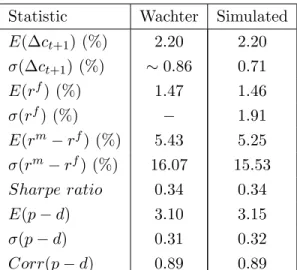
Tab. 3 - Comparison between simulation results from Wachter (2005).
Taking into account the fact that in a computer simulation there are many variables that we cannot match exactly, for instance: virtual random machine used in normal
vt+1 draws, decimal number approximation rules and so many others issues that make two computer simulations different from one another, we do not believe that program errors underlie the divergence that we found withb <0.Our program seems appropriate as we can see for its ability to reproduce finely the results in Campbell and Cochrane
(1999) and Wachter(2005).
Unfortunately, we do not have a reasonable explanation as of why we cannot reach finite values for the price-consumption ratio when interest rates are increasing in st.
Technically, by focusing on (24) one can see that the absolute value of λ(st) drives
positively the pricing kernel volatility. We can see in expression (10) that a negative
bdecreases the steady-state consumption surplus ratioS and, therefore, reduces Smax. Thus, the state-variable grid is filled with lower values. Given that λ is decreasing in
st, the sensitivity function will be higher than when a positive bis set on consumption
surplus grid points raising the stochastic discount factor volatility. How this increased volatility produces a divergence of our calibration procedure is of as this moment still not understood.
In another effort to understand the computational problems with b < 0, we have used an approach which is similar to the one proposed by Campbell and Cochrane
(1995), footnote 10. When we impose b < 0, the risk free rate is pro-cyclical and a linear increasing function of consumption surplus. In this case, if we fix an upper bound for the risk-free rate,20 we were able to find a closed expression forb in terms of γ,φ,
20
σv,r0f and the upper bound using (14) as follows:
rf(smax) =r0f−b[smax−s]≤rupper bound.
We then created three grids for (γ, φ, σv) 21 and used all possible combinations of
these parameters to find which ones have implied negative values for b. Our outcomes point to the fact that there is a very narrow range of parameters (0,98%) that delivers
b < 0. Moreover, all parameters combinations which yielded b < 0 displayed φ = 1, implying that the consumption surplus is a random-walk. This feature creates many difficulties to accommodate asset pricing phenomena other than the one the model is aiming at matching.
These results reinforce our perception that Campbell and Cochrane’s consumption-based model does not deal with pro-cyclical interest rates, at least in a well-behaved way, i.e. with φ < 1. To overcome this difficulty, Verdelhan (2009) proposed an
ad hoc approach to the original external habits model, which consists in making the sensitivity function,λ, described in (9), constant, at least during the price-consumption ratio computation from (16). The approach and its consequences will be the issue of our next subsection.
3.6 Verdelhan’s assumption
How is it possible to reconcile our negative results with Verdelhan’s well succeeded use of Campbell and Cochrane’s approach? That is, how did Verdelhan succeed in finding a finite value for the consumption-price ratio while at same time imposingb <0? The answer lies in the sensitivity function, λ(st). To find a closed form expression for the
risk-free volatility,Verdelhan(2009) assumes thatλ(st)≈λ(s), i.e.,λ(st) is a constant.
With a constant λno divergence problem arises and we can calibrate the model.22 After finding an appropriate price-consumption ratio, we release the sensitivity functionλin the simulations to vary as the original model does. In this manner, we are ensuring that risk free rate is pro-cyclical and, consequently, the UIP slope coefficient in simulated data is negative. In contrast, with a fixed λ, the risk fee rate is driven by rtf =−γ(1−φ)(st−s) +κ, where κ≡ −lnδ+γg−.5(γσv)2(1 +λ(¯s))2.Because
γ(1−φ) > 0, rft is still decreasing in st, the model would not generate a negative
βU IP. Also, fixing λ in simulation stage implies that risk premium no longer varies
21We estabilished grids for (
γ, φ, σv) using 50 points equally-spaced, respecting each one of the
following intervalsσv(%)∈[0,10]; γ∈(0,20];φ∈[0,1] and setrf0 at 0,9%. 22
Note,that, if one does not impose constancy of λ, λ(.) exhibits significant variation in st. For
counter-cyclically. This can be verified by examination of the Sharpe ratio expression for risky asset returns, (15).
To summarize, the procedure is potentially problematic because we are computing the price-consumption ratio under a stochastic discount factor that leads to anti-cyclical risk free rates although we intend to set interest rates pro-cyclically. We guess that this shortcut may generate inconsistencies for the model, mainly in realized equity returns that are driven by price-consumption’s time series.23
Instead of focusing on this potential source of inconsistencies we shall focus on other aspects of the model’s output. So, we pursue the strategy of fixingλin the calibration part of the exercise, and letting it vary in the simulations.
By running the calibration parameters from table II of his working paper, our program has been successful in reproducing his simulation results. Verdelhan draws 10,000 endowment shocks to create artificial quarterly data. Unfortunately, we do not know which state variable grid format was assumed in his working paper, thus little differences between his results and ours could happen at his parameters set.24
Verdelhan (2009)’s 25
Calibration parameters Verdelhan Statistic Verdelhan Simulated
g 2.12 E(∆ct+1) (%) 2.13 2.13
σv 1.02 σ(∆ct+1) (%) 1.04 0.84
rf 1.36 E(rf) (%) 1.65 1.40
φ 0.96 σ(rf) (%) 2.54 2.35
γ 2 E(rm−rf) (%) 3.98 3.93
b −0.01 σ(rm) (%) 8.72 13.62
Implied parameters Sharpe ratio 0.46 0.29
δ 1.00 E(p−d) 3.44 3.60
S 0.07 σ(p−d) 0.49 0.49
Smax 0.12 Corr(p−d) 0.97 0.97
23
Realized equity returns are computed as follows
Rt=
Ct+1
Ct
Pt+1
CT+1(st+1)
Pt
Ct(st)
,
so, any price-consumption inconsistency will affect realized returns.
24How much the use of different grids could change simulation results in this framework may be seen
inWachter(2005). The author uses 3 different grid types and summarizes her simulation results in tables 2 and 3 where great differences can be seen.
25
Notice that the difference in simulated consumption growth deviations displayed here and in
Tab. 4 - Comparison between simulation results from Verdelhan (2008) working paper and our computational calculations at same annualized calibration parameters set.
[Fig. 1 - Price-consumption ratio with Verdelhan parameters]
Our numerical exercise seems to match all results fromVerdelhan(2009), but equity returns volatility, and, consequently, the Sharpe ratio. However, we ought to highlight the low numbers of draws used by Verdelhan (10,000), which can make such results less reliable. To see this, we ran the model with the same calibration parameters used in latter comparison exercise but different seeds (See footnote 13). There are significant differences in such results as one can see in table 5. Whether one is matching or not the results becomes a more fuzzy matter.
Statistics Verdelhan seed1 seed2 seed3 seed4 seed5
E(∆ct+1) (%) 2.13 2.10 2.06 2.10 2.12 2.15
σ(∆ct+1) (%) 1.04 1.04 1.02 1.03 1.02 1.02
E(rf) (%) 1.65 1.13 0.72 0.99 1.24 1.93
σ(rf) (%) 2.54 2.07 2.51 2.51 2.32 1.47
E(rm−rf) (%) 3.98 4.32 5.10 4.66 4.17 2.82
σ(rm) (%) 8.72 14.08 14.49 13.78 13.48 12.02
Sharpe ratio 0.46 0.31 0.34 0.34 0.31 0.25
E(p−d) 3.44 3.53 3.44 3.51 3.57 3.72
σ(p−d) 0.49 0.49 0.54 0.55 0.52 0.47
Tab. 5 - Comparison between simulation results from Verdelhan (2008) working paper using 10,000 draws for consumption artificial data with different random seeds.
Nevertheless, the equity returns volatility found in simulations are consistently higher than his. Apparently, this is the only difference between the results in exercises using our algorithm and those elsewhere, given that we have succeeded in replicating
Campbell and Cochrane (1999) and Wachter (2005) results and almost all statistics from Verdelhan’s paper.
Now, assuming that λis constant and equal to its steady-state value, λ(s), allows us to calibrate the model and match the US real data.26 The parameter values and simulation results are described in tables 6, below.
26Setting
λ(st) = λ(s) is just an intuitive choice. Any other constant value, ¯λ, results in model
convergence. However, the choice of ¯λ affects dramatically the equity returns volatility. Indeed, for
Calibration parameters Statistic Real data Simulated
g 2.19 E(∆ct+1) (%)∗ 2.21 2.21
σv 2.02 σ(∆ct+1) (%)∗ 1.73 1.73
rf 0.98 E(rf) (%)∗
1.02 1.02
φ 0.931 σ(rf) (%) 2.96 2.16
γ 2 E(rm−rf) (%)∗
6.27 6.27
b −0.01 σ(rm−rf) (%) 15.15 17.32
Implied parameters Sharpe ratio 0.41 0.36
δ 0.95 E(p−d) 3.33 3.11
S 0.095 σ(p−d) 0.44 0.45
Smax 0.156 Corr(p−d) 0.915 0.93
Tab. 6 - Annualized calibration parameters set and simulation results chosen to match 1947-2004 US consumption, price and equity real data. Statistics that calibration parameters were chosen to
replicate.
The UIP coefficients we found confirms that the model delivers a consistent negative bias, whatever correlation between consumption processes of different nations is used. Therefore, the ad hoc Campbell and Cochrane model version proposed by Verdelhan is able to reproduce the FPP. Its values are summarized below.
UIP Coefficients
ρi βU IP ρi βU IP
-1.0 -3.2444 0.9 -4.4325
-0.9 -3.3499 0.8 -4.8277
-0.8 -3.4146 0.7 -5.0623 -0.7 -3.4911 0.6 -5.0707
-0.6 -3.5485 0.5 -4.9533
-0.5 -3.6016 0.4 -4.8047 -0.4 -3.6726 0.3 -4.6212
-0.3 -3.7593 0.2 -4.4344 -0.2 -3.8693 0.1 -4.2607
-0.1 -3.9948 0.0 -4.0883
Tab.7 - Respective UIP coefficients in relation toρi. All values are significant under an 95% confidence interval. The level coefficientαwas statistically null in every regression.
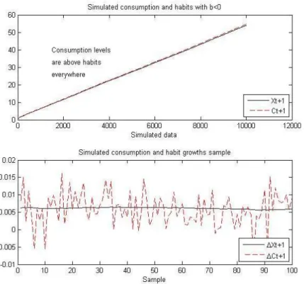
In their original paper,Campbell and Cochrane(1999) built the sensitivity function
λto reach 3 main goals: i)to make risk-free rate linear in the state variable st,ii) to
guarantee that habits are always lower than consumption, and; iii) to impose a non-negative co-movement between habits and consumption. The first objective is attained and can be seen in (14). For our calibration parameters, the latter two objectives are intact as can be seen in figure below. So, up to this moment, imposing a constant sensitivity function does not hurt the stated goals ofCampbell and Cochrane (1999).
[Fig.2 - Consumption and Habits]
3.7 Real bond yields
Nevertheless, impose pro-cyclical interest rates to match the forward discount anomaly in habits formation framework results in a detachedness between the average slope of the real yield curve delivered by model’s simulation and that observed in data.
Wachter (2006), like us, used Campbell and Cochrane external habits model to fit main features of the US nominal and real term structure of interest rates. She pointed out that under a positive b, i.e. when intertemporal substitution effects dominates precautionary savings effects in investor preferences, this model generates a positive real bond premia that increases with maturity. Hence, an upward-sloped yield curve, a feature which Boudoukh et al.(1999) have found support in real data, is generated by the model whenb >0.
As mentioned in Andersen and Lund (1996), inspection of historical U.S. interest rates reveals that the real yield curve tends to be upward-sloping and quite steep at the short end (0 to 5 years), while it is relatively flat for maturities in excess of 5 years. To check this observation in more recent data, figure 3 displays the real yields at 2-yr and 20-yr maturities for the period that runs from Apr/99 to Jan/04.27
[Fig. 3 - Real Yields]
To understand the link between the sign ofband the slope of the real yield curve we followWachter (2006) and write the standing representative investor’s Euler equation in the covariance form,
E(Rn,t−R1,t) =−Cov(Rn,t−R1,t, Mt)
σ(Mt)
E(Mt)
. (27)
27
Return at t on a bond maturing n periods in the future is Rn,t, the real short-term
interest rate is the one-period maturity returnR1,t and Mt is the pricing kernel.
The reason why this model generates a positively sloped yield curve is the combina-tion of two facts. First, the fact that bonds returns move in the opposite direccombina-tion from short term returns. Second, the fact that, withb >0,short term returns is negatively related to st,as one can see in (14).
Adjusting a positive b and calibrating the model to match real data we were able to reproduce an upward-sloping real yield curves for 1-year and 5-year bonds coincid-ing with Wachter (2006) and Andersen and Lund (1996) findings. These curves are presented below.
[Fig. 4 - Bond yields withb >0]
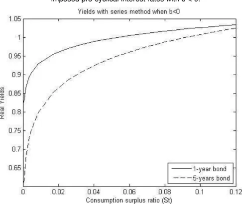
Turning back to our calibration parameters, i.e with b < 0, the model attain the following yield curves for same long-term bonds
[Fig. 5 - Bond yields withb <0]
In figure 5 we have a downward-sloping real yield curve with negative values. Using the symmetrical argument discussed above in case b > 0, the pro-cyclical behavior of interest rates results in a positive covariance between economic cycles and short term interest rate. Since bond returns move in opposite direction from the short term interest rate, when economy goes badly bond returns are higher. This behavior brings real bonds closer to insurance assets. Then, investors demands smaller risk premia or even negative to hold them. Because long-term bonds have smaller expected returns than if there were no risk premia, they must have smaller yields.
This real yield curve behavior contradicts the well documented empirical statements discussed before. The reader can find out more about this in Mishkin (1990) and
Piazzesi and Schneider(2006).
4
Conclusion
inca-interest rates were imposed in our calibration process. This outcome is strengthened by the lack of other works in literature that have used such model with pro-cyclical risk-free rates.
In a recent work, Verdelhan has had success using Campbell and Cochrane’s model to reproduce FPP findings in exchange markets calibrating it for industrialized economies. In the same way, our paper could match real data for US economy and reply the styl-ized fact of a negative UIP slope coefficient. However, this triumph is attained at some costs.
First, the shortcut proposed by Verdelhan to deal with the difficulties in the cal-ibration stage may lead to inconsistencies on the model’s time series, given that the price-consumption ratio is computed under an anti-cyclical environment. We did not explore this path so we do not provide any evidence of inconsistencies.
Another notable cost, not necessarily due Verdelhan’s shortcut, is the real yield downward-sloped shape delivered by the model when pro-cyclical risk free rates are imposed. It is well-known in literature that real yields almost always display an upward-sloping curve or a humped curve, but only seldom a downward-sloped, whilst here this shape shows always under pro-cyclical interest rate assumption.
Campbell and Cochrane’s consumption-based model seems not to be able to repro-duce simultaneously stylized facts in bond markets and in exchange markets because pro-cyclical interest rates must be settled to match the forward discount anomaly. Our results are not very conclusive, however, since we used Verdelhan’s shortcut. Un-fortunately, as of this moment we do not have a satisfactory explanation as of why the price-consumption ratio lack of convergence during original model’s solution when
b <0 is imposed. We know that there are definitely parameter values that can lead to non-convergence.
References
Abel, Andrew B., “Asset prices under habit formation and catching up with the Joneses,” The American Economic Review, 1990, pp. 38–42. 8,9
Andersen, T.G. and J. Lund, “Stochastic volatility and mean drift in the short rate diffusion: sources of steepness, level and curvature in the yield curve,” Manuscript, Northwestern University, 1996. 26,27
Bacchetta, P. and E. Van Wincoop, “Can information heterogeneity explain the exchange rate determination puzzle?,” American Economic Review, 2006, 96 (3), 552–576. 5
Backus, D.K., S. Foresi, and C.I. Telmer, “Interpreting the forward premium anomaly,” Canadian Journal of Economics, 1995, pp. 108–119. 5
Bekaert, G., “The time variation of risk and return in foreign exchange markets: A general equilibrium perspective,” Review of Financial Studies, 1996, pp. 427–470. 5
, R.J. Hodrick, and D.A. Marshall, “The implications of first-order risk aversion for asset market risk premiums,”Journal of Monetary Economics, 1997,40(1), 3–39.
5
Boudoukh, J., M. Richardson, T. Smith, and R.F. Whitelaw, “Ex ante bond returns and the liquidity preference hypothesis,”Journal of Finance, 1999, pp. 1153– 1167. 26
Campbell, John Y. and John H. Cochrane, “By force of habit: A consumption-based explanation of aggregate stock market behavior,” Technical Report 4995 1995.
9,21
and , “By force of habit: A consumption-based explanation of aggregate stock market behavior,” Journal of political Economy, 1999, 107 (2), 205–251. 1,2, 8, 9,
11,18,19,20,21,24,26,27
Coakley, J. and A.M. Fuertes, “Exchange Rate Overshooting and the Forward Premium Puzzle,” Technical Report, working paper, University of Essex 2001. 5
Cochrane, John H.,Asset pricing, Princeton University Press, 2001. 14
Engel, Charles, “The forward discount anomaly and the risk premium: A survey of recent evidence,” Journal of Empirical Finance, 1996,3 (2), 123–192. 5,6
Fama, Eugene F., “Term-structure forecasts of interest rates, inflation and real re-turns,” Journal of Monetary Economics, 1990, 25(1), 59–76. 17
Froot, K.A. and J.A. Frankel, “Forward discount bias: Is it an exchange risk premium?,” The Quarterly Journal of Economics, 1989, pp. 139–161. 5
Grossman, Sanford J. and Robert J. Shiller, “The determinants of the variability of stock market prices,” The American Economic Review, 1981, pp. 222–227. 6
Hansen, Lars P. and Robert J. Hodrick, “Forward exchange rates as optimal predictors of future spot rates: An econometric analysis,” The Journal of Political Economy, 1980, 88(5), 829. 4
Hodrick, Robert J.,The empirical evidence on the efficiency of foward markets and futures foreign exchange markets, Harwood, Chur, 1987. 3,4,5
Kandel, S. and R.F. Stambaugh, “Expectations and volatility of consumption and asset returns,” Review of Financial Studies, 1990, pp. 207–232. 6
Kocherlakota, Narayana R., “The equity premium: It’s still a puzzle,” Journal of Economic Literature, 1996, pp. 42–71. 6
Lustig, H. and A. Verdelhan, “The cross section of foreign currency risk premia and consumption growth risk,” American Economic Review, 2007, 97 (1), 89–117.
12
Lustig, Hanno and Adrien Verdelhan, “Investing in foreign currency is like bet-ting on your intertemporal marginal rate of substitution,” Journal of the European Economic Association, 2006, 4(2-3), 644–655. 12
Ma, A., “Macroeconomic Fundamentals and the Forward Discount Anomaly,” draft, 2006. 18
Macklem, Tiff, “Forward exchange rates and risk premiums in artificial economies,”
Journal of International Money and Finance, 1991, 10(3), 365–391. 5
Mehra, Rajnish and Edward C. Prescott, “The equity premium in retrospect,”
NBER working paper, 2003. 6
Mishkin, F.S., “Yield curve,” NBER Working Paper, 1990. 27
Moore, M.J. and M.J. Roche, “Solving exchange rate puzzles with neither sticky prices nor trade costs,” Manuscript, Queens University Belfast, School of Manage-ment and Economics, 2007. 6
Piazzesi, M. and M. Schneider, “Equilibrium yield curves,”NBER Macroeconomics Annual, 2006, 21(1), 389–442. 27
Shiller, Robert J., “Do stock prices move too much to be justified by subsequent changes in dividends?,” The American Economic Review, 1981, pp. 421–436. 6
Taylor, M.P., “The economics of exchange rates,” Journal of Economic literature, 1995, pp. 13–47. 3
Verdelhan, Adrien, “A habit-based explanation of the exchange rate risk premium,”
Working paper, 2009. 1,2,6,18,22,23,24
Veronesi, Pietro and F. Yared, “Short and long horizon term and inflation risk premia in the US term structure: Evidence from an integrated model for nominal and real bond prices under regime shifts,” CRSP Working Papers, 1999. 17
Wachter, J.A., “Solving models with external habit,”Finance Research Letters, 2005,
2 (4), 210–226. 11,18,19,20,21,23,24
Appendix - Figures
Figure 1 – Simulated price-consumption ratio with Verdelhan (2009)’s working paper parameters.
Figure 3 – The US Treasury real yield curve for maturities between 2-yr and 20-yr. Data are from US Federal Reserve daily yields between April/99 and Jan/04.