Stochastic Simulation of the Exchange Rate

(1)

The Annals of “Dunarea de Jos” University of Galati

Fascicle I - 2007. Economics and Applied Informatics. Years XIII - ISSN 1584-0409

117

Stochastic Simulation of the Exchange Rate

Corina SBUGHEA

sbughea@yahoo.com

“Dunărea de Jos” University of Galaţi

Anamaria ALDEA

Academy of Economic Studies - Bucharest

Abstract. This paper aims to illustrate the turbulent processes from financial markets, using stochastic simulation tools for this. In order to achieve this goal, we chose a suggestive model of the exchange rate behaviour, proposed by De Grauwe and Grimaldi. Having at our disposal the modelling facilities offered by EViews software, we managed to trace some significant trajectories for the actual behaviour of the exchange rate, which are consistent with the conclusions reached by the authors of the model.

Keywords: behavioral finance, rational expectations, fundamental exchange rate, non-fundamental equilibrium

1. Introduction

A long time, most macroeconomic studies were based on the assumption that market actors behave rationally. This type of agents is assumed that always act in order to continuously maximize their utility. It is said that the forecasts made by these agents are rational, if they take into account all available information, even that which derives from the structure of the functional dependence of variables, and they will not make systematic errors in anticipation of future values of the variables. According to Efficient Market Hypothesis (EMH), prices are formed in such a way to reflect all public information (both fundamental and price history are discounted). So, the prices change only when new information appears. Moreover, in an efficient market, speculation can not be made because, not only do the prices reflect all available information, but the large number of investors will make sure that the prices are fair (Peters, 1996). But the empirical evidence of the foreign exchange market contradicts the rational expectations and efficient market hypothesis. In fact, the agents may not know how to interpret all the available information and may move according to trends, thus adjusting their current actions according to past information.

An alternative model was presented by De Grauwe and Grimaldi (2006). They started from the observation that the information is too complex so no single agent can understand it entirely. Because agents are aware that they can not perceive the full complexity of market mechanisms, they will form different strategies that are not consistent with rational expectations model. Thus the authors of the model assumes that agents act in two stages. The first step is choosing a simple forecasting rule, called heuristic rule, which uses only parts of the entire set of the available information on the market. In the second stage, they will check whether the rule applied was efficient, comparing it with other rules used by other agents. If they find a more effective rule, they will use it in the next period. But if their rule has provided the highest profit, they will keep it also in the following period. This is called by the authors a trial and error learning strategy, because the agents will get to know the market, by trying different rules.

(2)

118

profitable. But they are limited to only choose between simple rules. Thus, the authors characterize the behavior of agents as being limited rational, ie “boundedly rational”, like it was first proposed by Simon in 1955, becoming one of the basic concepts of “behavioral economics”.

2. De Grauwe and Grimaldi’s behavioural finance model of the exchange rate

Using these assumptions, De Grauwe and Grimaldi developed a simple exchange rate model. They started by defining the concept of fundamental exchange rate as the level of the exchange rate, which corresponds to the equilibrium of the real economic system (which may be even the Purchasing Power Parity-value). The fundamental exchange rate, st, is supposed to be an exogenous

variable, wich behaves like a random walk without drift (we kept authors’s notations):

t t

t

s

*

=

*₋₁

+

ε

(1) where st is a white noise error variable.

They assumed that agents can use two types of simple forecasting rules. One type of forecasting rule will be named fundamentalist, and the agents who are using this rule will be called fundamentalists. The second type will be named the chartist rule and the agents who use this rule will be named chartists or analysts who are using the technical rule. It is considered that the fundamentalists agents are aware of the fundamental level of the exchange rate, and they can compare it with the current market rate. They will expect the exchange rate to tend to the fundamental level, so that adjustment will be made through a negative feedback loop:

(2)

In equation (2), Ef,t is the anticipation made in period t by the fundamentalists using information up

to time t, st is the market exchange rate at the moment t, ∆st+1 is the change in the exchange rate,

and ψ > 0 is a coefficient expressing the speed with which the fundamentalists expect the exchange rate to reach the fundamental level.

Regarding the second category of agents, they will observe the previous rate changes and they will extrapolate ahead. So, the chartists will follow a positive feedback rule, by extrapolating only last period’s exchange rate movement, into the next interval of time:

t t

t

c

s

E

_,

(

∆

₊₁

)

=

β

∆

(3)

In previous equation, Ec,t is the forecast made by the chartists using information up to time t, and

β

(

β

∈(0,1)) is the parameter that measures the extent to which chartists extrapolate the past movements of the exchange rate. These technical analysts are considered by the authors as being noise traders, because they do not relate in any way to the fundamental exchange rate, which is considered the equilibrium level.

All agents on the market are using in a time interval, one of these two rules. Then they compare the efficiency of the used rule, being willing to move to the other one, if that was not profitable. This idea was implemented using concepts of discrete choice theory. Thus the set of all market actors is divided into these two groups, fundamentalist and chartist, using risk adjusted functions of the relative profitability of their forecasting rules:

' , ' , ' , , exp exp exp t c t f t f t f w

γπ

+

= (4)

)

(

)

(

1 *

,t t t t

f

s

(3)

119 (6) ' , ' , ' , ,

exp

t c t f t c t c

w

γπ

+

=

(5)

where wf,t and wc,t are the weights of the fundamentalists, respectively the chartists, on the market,

thereby wf,t + wc,t =1. The variables '

,t f

π

and

π

_c'_,_t are the adjusted profits of the both types of forecasting rules in period t, , 2,

'

,t f t ft

f

π

µσ

π

=

−

and , 2,

'

,t ct ct

c

π

µσ

π

=

−

, where

π

_f,_t and

π

c,tare the profits made by each rule, and

σ

2_f_,_t and

σ

_c2_,_t are the risks the two categories of agents are exposed to, by using these rules. The risks are expressed as error variables and the level of risk aversion is introduced through parameter μ.

In equations 4 and 5, the parameter γ reflect the intensity with which the chartists and fundamentalists are currently reviewing the rules they are using. Thus, a high value of γ, means that the agents are very sensitive to the adjusted profits of the two rules. If γ tends to infinity, all the agents choose the most profitable forecasting rule. In the opposite, if γ tends to zero agents are insensitive to the adjusted profits of the rules and the weights of fundamentalists and chartists are equal to 0.5.

The profits are defined as the earnings of investing $1 in the foreign asset, in one interval of time (for simplicity, we have not taken into account the correction with the interest rates):

]

)

(

sgn[(

]

[

₁ ₁ ₁

,

=

−

− − t

−

t−

i t t

t t

i

s

E

s

π

where











<

−

=

>

=

0 .

,

1

0 .

,

0

0 .

,

1 ]

sgn[

x

for

x

for

x

for

x

,

with i=c,f

Thus, when agents are expecting an increase in the exchange rate and this increase occurs, they

make a profit (per unit) equal to the observed increase in the exchange rate. But if instead the exchange rate decreases, they register a loss (per unit), which equals this decrease, because in this situation they invested in assets which have been devalued.The risk associated with each forecasting

rule is the forecast error, and agents take into account only the last period’s forecast error:

2 1

2

,

[

t

(

t

)

t

]

i

t

i

=

E

−

s

−

s

σ

(7)

The forecast at market level is obtained by aggregating the chartist and fundamentalist forecasts:

t t c t t t f t

t

s

w

s

w

s

E

∆

₊

=

−

ψ

−

+

,

β

∆

* ,

1

(

)

₍₈₎

The movement of the market exchange rate in period t+1 is equal with the market forecast made at time t, perturbed with a white noise type of error, at time t+1, which may include the information

that could not be anticipated at time t:

1 ,

* ,

1

(

)

+

=

−

+

∆

+

(4)

120

3. Stochastic simulation of the model in EViews

We defined the model in EViews by choosing Objects/ New Object...Model, and added one by one the equations, which can be identities or stochastic equations.

where sf is the fundamental rate, which is random generated using the normal distribution, s is the market exchange rate, Esf and Esc are the fundamental and chartist forecasts, wf and wc are the corresponding fractions of the population, pic and pif are the profits of the rules, and pifl and picl are the risk adjusted profits. The sgn function was defined using the default function @recode.

In EViews, a model can be simulated deterministically or stochastically. In case of the stochastic simulation, the equations of the model are solved so that they have residuals which match to randomly drawn errors. Optionally, the parameters and the exogenous variables of the model can also vary randomly. In this case, the software generates a distribution of results for the endogenous variables in every period. A stochastic simulation follows a sequence which has some differences from the deterministic one1:

■ The variables in the model are bound to series, so a temporary series is created for every calculated variable. For every tracked endogenous variable is created an additional serie in the work file which will hold the statistics.

1

(5)

121

■ The model is solved repeatedly for different draws of its stochastic components. If there are uncertainty coefficients in the model, then a new set of values is generated before each repetition. Every time, errors are generated for each observation in accordance with the residual uncertainty and the exogenous variable uncertainty in the model. The statistics for the tracked endogenous variables will be updated after each repetition, with the additional results.

We can select the algorithm that will be used to solve the model for one period, from the Solution algorithm box, which offers the following choices:

■ Gauss-Seidel: which is an iterative algorithm, that at each iteration solves each equation in the model for the value of its associated endogenous variable, keeping fixed the other endogenous variables.

■ Newton: which is also an iterative algorithm, where at each iteration is taken a linear approximation of the model, and then the linear system is solved to find a root of the model. It is considered that this method can solve a larger class of problems than Gauss-Seidel, but requires more resources, so has a much greater computational cost when it is applied to complex models.

(6)

122

Varying the parameters of the model, we can observe the evolution of the market exchange rate towards the fundamental rate.

The fundamental exchange rate has a random walk type of trajectory, as it contains a white noise error. In different simulation runs of the model, but using the same values for input parameters, it can be observed that the exchange rate deviates very often from the fundamental exchange rate (which corresponds to authors' conclusions):

Fig.1- Fundamental and market rate

So, the market exchange rate evolves differently from the fundamental rate. De Grauwe and Grimaldi separated these exchange rate movements in two regimes. In one regime the exchange rate follows the fundamental exchange rate closely, so they called these episodes “fundamental regimes”. The other type of behaviour is called “bubble” or non-fundamental regime, corresponding to the situations in which the chartists’ fractions tend to 1. The fundamental regimes occur, on the contrary, when the chartists’ weights are below 1.

(7)

123

Fig2. – Change in fundamental and market rate

The stochastic simulations of the market and fundamental exchange rates, for different values of γ are presented in Fig. 3. As the parameter γ measures the sensitivity of the switching rule to risk adjusted profits, is expected that, when γ has a greater value, agents will be very active in changing the forecasting rules according to their profitabilities. On the contrary, when γ has lower values, the agents do not take into account profits when choosing the rule.

These expectations are confirmed in the simulations from Fig. 3. So, for a greater γ, the market exchange rate moves away from the fundamental level, having almost all the time bubble regimes. Instead, for a lower γ, the market exchange rate converges in time to the fundamental level.

(8)

124

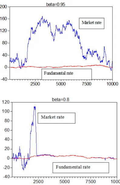
As the chartist are noise traders, is expected that the parameter β, which measures the degree of extrapolation in the technical forecasting rule, will have a great influence on the evolution of the market exchange rate. In Fig.4 can be seen that, when β has values close to 1, the exchange rate diverges strongly from the fundamental level, and when β decreases (but not so much) the market exchange rate converges in time to the fundamental rate.

Fig. 4 – Simulations for different values of β

Conclusions

(9)

125

real systems must take into account the large degree of uncertainty, therefore the simulations performed on stochastic models are closer to the actual behavior of systems.

References

[1] Anderson S., de Palma A., Thisse J.-F., Discrete Choice Theory of Product Differentiation, MIT Press, Cambridge, Mass. 1992

[2] Brock W., andHommes C., A Rational Route to Randomness, Econometrica,65, 1059-1095,1997

[3] Brock, W., and Hommes, C., Heterogeneous beliefs and routes to chaos in a simple asset pricing model,

Journal of Economic Dynamics and Control, 22, 1235-1274,1998

[4] Calvo G., and Mendoza E., Rational Contagion and the Globalization of Securities Markets,1999,

http://www.bsos.umd.edu/econ/ciecrp6.pdf.

[5] Calvo G., Capital Market Contagion and Recession: An Explanation of the Russian Virus, University of

Maryland, College Park. Processed, 1998

[6] Corsetti G., Pesenti P., and Roubini N., What Caused the Asian Currency and Financial Crises? A

Macroeconomic Overview., Processed (September), New York University,1998

[7] DeGrauwe P., Grimaldi M., The Exchange Rate in a Behavioral Finance Framework, Princeton

University Press, 2006

[8] Diamond D. W., and Dybvig P.H., Bank Runs, Deposit Insurance, and Liquidity, Journal of Political

Economy,91: 401-19, 1983

[9] Dooley M., A Survey of Literature on Controls Over International Capital Transactions, IMF Staff

Papers 43(4):639-87, 1996

[10] Dornbusch, R., Expectations and exchange rate dynamics, Journal of Political Economy 84, 1976

[11] Edison H., and Reinhart C., Stopping Hot Money, 1999, http://www.puaf.umd.edu/papers/reinhart.htm.

[12]Eichengreen B., and Mathieson D., Hedge Funds and Financial Market Dynamics, Occasional Paper

181, International Monetary Fund, Washington, D.C, 1998

[13] Hood R., Malaysian Capital Controls, World Bank, Washington, D.C., 2000

[14]Ito T., The Development of the Thailand Curency Crisis: A Chronological Review, Hitotsubahi

University, 1998

[15]Kaminsky G., and Reinhart C., On Crises, Contagion, and Confusion, Journal of International

Economics 51, 2000

[16]Kaminsky G., and Reinhart C., The Twin Crises: The Causes of Banking and Balance-of-Payments

Problems, American Economic Review 89, 1999

[17]Krugman P., A Model of Balance-of-Payments Crises, Journal of Money, Credit, and Banking 11:31125,

1979

[18]Krugman P., Saving Asia: It's Time to Get Radical, Fortune Investor 7:33-8, 1998b

[19]Mishkin F.S., Financial Policies And The Prevention Of Financail Crises In Emerging Market Countries,

, NBER, Working Paper 8087, 2001

[20]Mishkin F.S., Understanding Financial Crises: A Developing Country Perspective, Annual World Bank

Conference on Development Economics, 1996a

[21]Obstfeld M. and Rogoff K., Foundations of International Macroeconomics, MIT Press, Cambridge,

Mass. 1996

[22]Obstfeld M., Rational and Self-Fulfilling Balance of Payments Crises, American Economic Review

76:72-81, 1986

[23]Peters E., Chaos and order in the Capital Markets, John Wiley & Sons, 1996

(10)

126 Sons, 1994

[25]Perry G., Lederman D., Financial Vulnerability, Spillover Effects and Contagion: Lessons from the Asian Crises for Latin America, Washington, D.C.: World Bank, 1998

[26]Radelet S., Sachs J., The East Asian Financial Crisis: Diagnosis, Remedies, Prospects, Brookings Papers on Economic Activity 1: 1-90. 1998a

[27]Radelet S., Sachs J., The Onset of the East Asian Financial Crises, NBER Working Paper 6680, 1998b

[28]Simon H. A., A Behavioral Model Of Rational Choice, The Quarterly Journal of Economics, Vol. 69, No.

1, 99-118. Feb., 1955.

[29]Taylor M., and Allen H, The Use of Technical Analysis in the Foreign Exchange Market, Journal of

International Money and Finance, 11, 304-14, 1992