Anomalous gauge couplings from composite Higgs and warped extra dimensions

JHEP03(2014)102

Received_: January 11, 2014

Accepted_{: February 26, 2014} Published_{: March 24, 2014}

Anomalous gauge couplings from composite Higgs

and warped extra dimensions

Sylvain Ficheta and Gero von Gersdorffb

a_{International Institute of Physics, UFRN,}

Av. Odilon Gomes de Lima, 1722, Capim Macio, 59078-400, Natal-RN, Brazil b_{ICTP South American Institute for Fundamental Research,}

Instituto de Fisica Teorica, Sao Paulo State University, Brazil

E-mail: [email protected],[email protected]

Abstract: _{We examine trilinear and quartic anomalous gauge couplings (AGCs)} gener-ated in composite Higgs models and models with warped extra dimensions. We first revisit the SU(2)L×U(1)Y effective Lagrangian and derive the charged and two-photon neutral AGCs. We derive the general perturbative contributions to the pure field-strength opera-tors from spin 0, 1₂, 1 resonances by means of the heat kernel method. In the composite Higgs framework, we derive the pattern of expected deviations from typical SO(N) embed-dings of the light composite top partner. We then study a generic warped extra dimension framework withAdS5 background, recasting in few parameters the features of models

rele-vant for AGCs. We also present a detailed study of the latest bounds from electroweak and Higgs precision observables, with and without brane kinetic terms. For vanishing brane kinetic terms, we find that the S and T parameters exclude KK gauge modes of the RS custodial [non-custodial] scenario below 7.7 [14.7] TeV, for a brane Higgs and below 6.6 [8.1] TeV for a Pseudo Nambu-Goldstone Higgs, at 95% CL. These constraints can be re-laxed in presence of brane kinetic terms. The leading AGCs are probing the KK gravitons and the KK modes of bulk gauge fields in parts of the parameter space. In these scenarios, the future CMS and ATLAS forward proton detectors could be sensitive to the effect of KK gravitons in the multi-TeV mass range.

Keywords: _{Electromagnetic Processes and Properties, Beyond Standard Model, Field} Theories in Higher Dimensions, Technicolor and Composite Models

JHEP03(2014)102

Contents

1 Introduction 1

2 The effective Lagrangian 3

3 Anomalous gauge couplings in the broken phase 4

4 The generic loop contributions to L∂ ₇

5 Composite Higgs models and their holographic description 9

6 Integrating out a warped extra-dimension 13

6.1 The 5d framework 13

6.2 Contributions from KK gravity 17

6.3 Contributions from KK gauge modes 18

6.4 Contributions from KK-loops 18

7 Bounds from Higgs and electroweak precision measurements 19

8 Probing a warped extra dimension using anomalous gauge couplings 22

9 Conclusion 26

A The heat kernel coefficients 28

B Integrating out a warped extradimension at tree-level 29

B.1 KK gravity 29

B.2 KK gauge 31

1 Introduction

Several major facts like the gauge-hierarchy problem or the observation of dark matter suggest that physics beyond Standard Model of particles (SM) should be present in nature at a mass scale relatively close to the electroweak scale. However, in spite of naturalness arguments, the paradigm of a TeV-scale new physics is challenged by both direct LHC searches and by indirect observables like the LEP electroweak precision tests. In a scenario of new physics out of reach from direct observation at the LHC, one may expect that the first manifestations show up in precision measurements of the SM properties.

JHEP03(2014)102

interactions. This is a domain relevant for the CMS and ATLAS main detectors, and also for the future CMS and ATLAS forward proton (FP) detectors [1–3] whose construction may start in 2014.

Just like the couplings of other sectors of the SM, anomalous gauge couplings can be systematically analyzed through the effective Lagrangian framework. This approach relies on the assumption that the energy scaleEaccessible by the experiment is small with respect to the new physics mass scale Λ ,

E_≪Λ. (1.1)

This fundamental assumption allows one to describe any manifestation of new physics by local operators of higher dimension. The low-energy effective Lagrangian is written as the SM Lagrangian plus an infinite sum of these higher dimensional operators (HDOs),

Leff =LSM+ X

i

αi

ΛmiOi. (1.2)

For a given set of observables of interest (in our case, the anomalous gauge couplings), it is then sufficient to keep only the operators at the appropriate first orders of the expansion. By construction these operators capture the leading effects induced by the heavy new physics. In the present study, the observables of interest are the trilinear gauge couplings and quartic gauge couplings (TGCs, QGCs). As the FP detectors provide particularly good sensitivity to the process of diffractive photon fusion, we are going to limit our study to two photon QGCs. In order to describe the effects of new physics on TGCs and QGCs, it turns out that we have to keep dimension 6 operators for charged anomalous gauge couplings (CGCs) and dimension 8 operators for neutral anomalous gauge couplings (NGCs). Higher order effects in the observables will be of order O(E2_/Λ2_{, v}2_/Λ2_{) where E is the typical}

energy involved in the process. We will also keep some charged dimension 8 operators relevant for two-photon physics. Anomalous gauge couplings have already been studied from the effective Lagrangian point of view, see e.g. [4,5], and the recent review [6] and references therein.

In this paper we aim at going one step further, by mapping actual models of new physics onto the effective Lagrangian. In particular we investigate the effects of composite Higgs and of warped extra dimensions. Although we consider actual theories of new physics, we adopt an effective parametrization of the theories in order that our predictions cover the broadest range of possibilities and facilitate comparison with other approaches.

JHEP03(2014)102

in composite Higgs models. In section6 we study warped extra dimensions, including the case of brane gauge field (sometimes referred to as RS I) and the Randall-Sundrum model with bulk gauge fields, as well as the composite Higgs models via holography. Section 7 contains an update on the bounds from Higgs and electrowek precision tests on KK gauge modes and radion masses. In section 8 we present and discuss the anomalous couplings predicted in the warpedAdS5 framework, including the effect of the radion/dilaton and of

the KK gravitons. Section 9is devoted to our conclusions.

2 The effective Lagrangian

First we define the set of higher dimensional operators entering the effective Lagrangian eq. (1.2).1 _{The complete Lagrangian describing anomalous gauge couplings in the broken} phase, needed for phenomenology and experimental studies, will be derived in the next section. Throughout this paper we use the conventions of [8], including the mostly minus metric signature (+,₋,₋,₋). We limit the expansion of_Leff to order 8, such that

Leff =LSM+L(6)+L(8). (2.1)

The_L(6) piece induces the leading deviations to TGCs, while the_L(8)generates anomalous quartic NGCs.

The HDOs at a given order can be brought into an irreducible set, i.e. a basis, using the equivalence relations provided by integration by parts and equations of motion. There is a freedom in the choice of the particular basis.2 Here our dimension six basis is defined in such a way that (in renormalizable theories) the operators_OF F,OW3 are only generated

pertubatively at the loop level while the other ones can potentially be generated at tree-level. This particularly convenient basis has been already used in [9], is discussed more formally in [10], and is consistent with the general basis presented in [11]. We display below only the operators which will feed into anomalous gauge couplings, or will be closely related to their study. In particular, dipole operators and Yukawa-like dimension six operators are not shown.

The dimension six Lagrangian _L(6) contains the operators3

OD2 =|H|2|D_µH|2, O_D′ 2 =|H†DµH|2, (2.2)

OD =JH µa Jf µa , O′D =JH µY Jf µY , (2.3)

O4f =Jf µa Jf µa , O′4f =Jf µY Jf µY , (2.4) OWW =H†H(Wµνa )2, OBB =H†H(Bµν)2, OWB =H†WµνH Bµν, (2.5)

OW3 =εIJKW_µνI W_νρJW_ρµK. (2.6)

1_{It is sufficient to use the linearly realized SU(2)×U(1) Lagrangian, as the nonlinear realization tends}

to the linear one in the limitv≪Λ. See e.g. [7] for more details about anomalous gauge couplings in the nonlinear realization.

2_{Note that although the effects on the physical observables from different basis must be the same, they}

can appear in a rather different way. For example, a modification of theW propagator in a given basis may be recasted in a shift of the Fermi constant in another basis.

3_{The four fermion operatorsO}

4f andO′4f do not appear in the basis of ref. [9], as they can be eliminated

JHEP03(2014)102

J_fa µ=X ψL

1 2ψ¯Lγ

µσa

2 ψL J

Y µ f =

X

ψ

Yψψγ¯ µψ (2.7)

and

J_Ha µ= i 2H

†_σa←_D→µ_{H , J}Y µ H =

i 2H

†←_D→µ_{H (2.8)}

whereYψ is denotes the hypercharge.

The dimension eight Lagrangian relevant for neutral gauge couplings is [5]

L(8)= α1

Λ4D

µ_H†_D

µHDνH†DνH+α2 Λ4D

µ_H†_D

νHDνH†DµH

+α3 Λ4D

ρ_H†_D

ρHBµνBµν+

α4

Λ4D

ρ_H†_D

ρHWµνI WIµν+

α5

Λ4D

ρ_H†_σI_D

ρHBµνWIµν

+α6 Λ4D

ν_H†_D

ρHBµνBµρ+

α7

Λ4D

ν_H†_D

ρHWµνI WIµρ

+α8 Λ4B

µν_B

µνBρσBρσ+α9 Λ4W

Iµν_WI

µνWJρσWρσJ +

α10

Λ4W

Iµν_WJ

µνWIρσWρσJ

+α11 Λ4B

µν_B

µνWIρσWρσI +

α12

Λ4 B

µν_WI

µνBρσWρσI

+α13 Λ4B

µν_B

νρBρσBσµ+

α14

Λ4 W

Iµν_WI

νρWJρσWσµJ +

α15

Λ4 W

Iµν_WJ

νρWIρσWσµJ

+α16 Λ4B

µν_B

νρWIρσWσµI +

α17

Λ4 B

µν_WI

νρBρσWσµI . (2.9)

We limit ourselves to two-photon QGCs, such that by gauge invariance the operators_O1,2

cannot contribute.

3 Anomalous gauge couplings in the broken phase

In this section we revisit and expand the anomalous Lagrangian in the broken phase, i.e. expressed in terms ofFµν,Zµ,Wµ±, containing all leading contributions to anomalous TGCs and QGCs. One can distinguish two types of deviations, those correcting couplings already existing in the SM at tree-level, denoted by coefficientsκ, and those corresponding to new Lorentz structures, denoted by coefficientsλ,η,ζ. The Standard Model corresponds to takingκi →0, λi →0,ηi →0,ζi→0.

We organize the Lagrangian as

Leff =Lkin+LCGC+LNGC. (3.1)

The first term _Lkin contains the kinetic terms and no anomalous interactions. We write

it only to set up the conventions. The second term _LCGC contains the charged gauge

couplings, including the Standard Model ones. The third term_LNGC contains the neutral

gauge couplings, which do not exist in the SM at tree-level. One can further decompose the anomalous Lagrangians as

LCGC =LSMCGC,v+L∂CGC, LNGC=LvNGC+L∂NGC, (3.2)

JHEP03(2014)102

two regimes, the “broken phase” regime E < v in which the effect of the _L∂ Lagrangian in the observables can typically be neglected with respect to the effects of _Lv _{, and the} “unbroken phase” regimev < E <Λ where the effects of_L∂ dominate over the ones of_Lv. In the regime Λ< E the effective field theory prescription breaks down and our results do not apply.

The kinetic Lagrangian reads

Lkin =−

1 2Wˆ

+

µνWˆµν− − 1 4F 2 µν− 1 4Z 2 µν (3.3)

where we defined U(1)em covariant field strength

ˆ

W_µν+ =DµWν+−DνWµ+. (3.4)

where hereDis only covariant w.r.t. U(1)em. The kinetic term ˆWµν+Wˆµν− contains all U(1)em interactions between the photon and theW’s which are protected from any deviations. The LSMCGC,v piece reads4

LSMCGC,v = −ie(1 +κ1)FµνW

−

µWν+−igZ(1 +κ2)ZµνWµ−Wν+

−igZ(1 +κ3)[ ˆWµν+Wν−−Wˆµν−Wν+]Zµ−gZ2(1 +κ4)2 |Wµ+|2|Zν|2− |ZµWµ+|2

+1 4g

2

W(1 +κ5)2(Wµ−Wν+−Wµ+Wν−)2+η1WFµνFµνW+ρWρ−

+η₂WFµνFµσW+νWσ−, (3.5)

where in terms of the operator coefficients

κ1 = αW B

2t2

w

v2 Λ2 ,

κ2 =−

swcw (c2

w−s2w)

αWB

v2 Λ2 −

1 4(c2

w−s2w)

[α′_D2 +αD−α4f]

v2 Λ2,

κ3 =κ4=−

sw 2cw(c2w−s2w)

αWB

v2 Λ2 −

1 4(c2

w−s2w)

[α′_D2 +αD −α4f]

v2 Λ2,

κ5 =−

cwsw 2(c2

w−s2w)

αWB

v2 Λ2 −

c2_w 4(ˆc2

w−s2w)

[α′_D2+αD−α4f]

v2 Λ2

η₁W = m

2

W Λ4 (c

2

wα3+s2wα4+cwswα5)

η₂W = m

2

W Λ4 (c

2

wα6+s2wα7).

(3.6)

The _L∂_CGC piece reads

L∂CGC =λZ[igZZµν( ˆWνρ−Wˆρµ+ −Wˆνρ+Wˆρµ−)] +λγ[ieFµν( ˆWνρ−Wˆρµ+ −Wˆνρ+Wˆρµ−)] +ζ₁WFµνFµνW+ρσWρσ− +ζ2WFµνFνρW+ρσWσµ−

+ζ₃WFµνW_µν+FρσW_ρσ− +ζ₄WFµνW_νρ+FρσW_σµ− .

4_{Theκanomalous couplings are related to the customary parametrization of [12] followingκ}

γ= 1 +κ1,

κZ= 1 +κ2,g1Z= 1 +κ3. The SU(2)×U(1) gauge invariance implies in generalκ2=κ3−κ1s

2 w c2

JHEP03(2014)102

λZ =λγ = 3αW3 gΛ2

ζ₁W = Λ−4 4s_w2 α9+ 2c2wα11

ζ₃W = Λ−4 4s_w2 α10+ 2c2wα12

ζ₂W = Λ−4 4s_w2 α14+ 2c2wα16

ζ₄W = Λ−4 4s2_wα15+ 2c2wα17 .

(3.7)

The _Lv_NGC piece is

LvNGC=ηZ1FµνFµνZρZρ+ηZ2FµνFµσZνZσ (3.8)

with

ηZ₁ = m

2

Z 2 Λ4(c

2

wα3+s2wα4−cwswα5)

ηZ₂ = m

2

Z 2 Λ4(c

2

wα6+s2wα7).

(3.9)

Finally, the _L∂

NGC piece is5

L∂NGC=ζ1γFµνFµνFρσFρσ+ζ2γFµνFνρFρσFσµ +ζ₁γZFµνFµνFρσZρσ+ζ2γZFµνFνρFρσZσµ

+ζ₁ZFµνFµνZρσZρσ+ζ2ZFµνFνρZρσZσµ +ζ₃ZFµνZµνFρσZρσ+ζ4ZFµνZνρFρσZσµ,

with

ζ₁γ= Λ−4 _c4

wα8+s4w(c9+α10) +c2ws2w(α11+α12)

ζ₁γZ = Λ−4 ₋4swcw3α8+ 4s3wcw(α9+α10) + 2cwsw(c2w−s2w)(α11+α12) ζ₁Z = Λ−4 2c_w2s2_w(α8+α9+α10−a12) + (c4w+s4w)α11

ζ₃Z = Λ−4 4c_w2s2_w(α8+α9+α10−α11) + (cw2 −s2w)2α12

(3.10)

ζ₂γ= Λ−4 c_w4 α13+s4w(α14+α15) +c2ws2w(α16+α17)

ζ₂γZ = Λ−4 ₋4swcw3α13+ 4s3wcw(α14+α15) + 2cwsw(c2w−s2w)(α16+α17) ζ₂Z = Λ−4 _4c2

ws2w(α13+α14+α15−α17) + (c2w−s2w)2α16

ζ₄Z = Λ−4 2c_w2s2_w(α13+α14+α15−α16) + (c4w+s4w)α17 . (3.11)

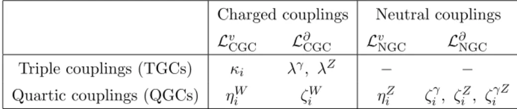
A summary of our notation for the many anomalous couplings can be found in table1. Before we close this section, let us comment on the validity of EFT and the experi-mental sensitivity. The operators_Oi are supposedly generated by a heavy particle of mass

5_{The neutral coefficients have been computed in [5]. We observe a discrepancy between our coefficients}

JHEP03(2014)102

Lv

CGC L∂CGC LvNGC L∂NGC

Triple couplings (TGCs) κi λγ, λZ − −

Quartic couplings (QGCs) ηW

i ζiW ηiZ ζiγ, ζiZ, ζiγZ

Table 1. Summary of our notation for the anomalous gauge couplings.

Λ, and hence EFT is valid as long as E _≪ Λ. In practice (i.e. at a hadron collider) the energy will be distributed over a certain range, but bounded from above by some Emax,

hence it is reasonable to only demand

Emax≤Λ, (3.12)

with the equality still being reasonably consistent with the EFT approach. Let us define the experimental sensitivity Λs

i to be the (say) 95% C.L. bound on the interaction (Λsi)−miOi. Clearly Λs is a function of Emax, and a given heavy particle can be constrained only if

Λ_≤(αi)

1

mi _Λi

s(Emax). (3.13)

One can obtain a rough estimate of the sensitivity by combining eq. (3.13) with the EFT criterion eq. (3.12). This implies that Λi

s(Emax)≥(αi)−

1

mi_{Emaxin order for the experiment}

to be sensitive to a particular New Physics effect. The ratio Emax/Λis(Emax) is a measure

of how strongly coupled new physics has to be in order to be tested experimentally by the effective interaction _Oi.

4 The generic loop contributions to L∂

We observed above that the_L∂ piece of the effective Lagrangian dominates in thev < E < Λ regime, i.e. the _Lv piece can be neglected. This implies that the effective Lagrangian is not only U(1)em symmetric, but also SU(2)L×U(1)Y symmetric in this regime. Given that _L∂ contains only pure gauge operators, one can then make the crucial observation that any one-loop diagram contributing to_L∂ has all its vertices fixed by gauge-invariance. As a consequence, any perturbative contribution to_L∂ _{is fixed once the quantum numbers} and the mass of the states running in the loop are specified. This allows us to provide formulas to easily compute _L∂ in any model of new physics. We employ the heat kernel method to derive these loop contributions. Some elements of the derivations are collected in appendixA.

Let us consider a (real) heavy vector Xµ with mass mX charged under SU(2)L× U(1)Y ≡ GEW. In order to obtain a consistent Lagrangian, we will write the theory as

a nonlinearly realized theory of a larger, not necessarily simple, gauge group G, i.e. we assume that the heavy gauge bosons live in the coset G/GEW. The interactions of this

heavy vector with the electroweak gauge bosons Vµ= (Wµ, Bµ) are described by

L=₋1 4( ˆX

˜

a µν)2−

1 4(V

a µν)2−

c 2X

˜

a µX

˜

b νf˜a

˜_bc

JHEP03(2014)102

G split into those of GEW, fabc, and the coset f˜a˜bc which form a (in general reducible)

representation of GEW. The ˆXµνaˆ is the GEW covariant field strength,

ˆ

X_µν˜a =DµXνa˜−DνXµa˜ (4.2)

The coefficientccould in general be arbitrary, but at leading order is given by c=g, if we assume that there is at least a small hiearchyf _≪Λ between the cutoff of the theory and the scalef of the breakingG_→GEW. As typical example – that also serves as a model for

the first Kaluza Klein (KK) resonances of an extra dimensional theory – consider a two-site model with gauge groupG=G′_×GEW withG′ ⊃GEW. Then the cosetG/GEW contains

precisely the adjoint ofGEW and the representations appearing in the cosetG′/GEW, that

is, formally all the representations of the decomposition G′ _→G

EW appear once.

We work in the Feynman-background gauge, in which there is no mixing between spin-1 and Goldstone degrees of freedom, the latter being degenerate in mass with the corresponding gauge fields. The ghosts contribute as an adjoint with multiplicity ₋2, and they are also degenerate in mass. Then, we can compute the contribution of each irreducible GEW representation ta_X appearing in the decomposition underG→ GEW to the one-loop

effective action as

S_effX = i

2tr log −[D

2_+m2

X]ηµν+ 2ig VµνataX

+ i

2(1−2) tr log −D

2

−m2_X

(4.3)

where the last term is the sum of Goldstone and ghost contributions. Everything is background-covariant w.r.t.Vµ. One might observe that the massive vector in this gauge is thus a trivial generalization to the massless one, the only differerence besides the nonzero mass being the Goldstone contribution.

Apart from the generic heavy vector, let us also consider a real scalar and a Dirac fermion with masses mS, mf transforming under respectively tSa, taf of GEW. The corre-sponding contributions are

S_effS = +i

2tr log −D

2_−m2

S

, (4.4)

S_efff = ₋i

2tr log −D

2_−m2

f +g SµνVµνataf

, (4.5)

where the Lorentz generators are defined asSµν = ₄i[γµ, γν]. Denoting the generators of a representation of a particle with spin s= (0,1₂,1) asTa _={ta

S, taf, taX}, the three and four field–strength operators will be respectively proportional to the traces of three and four generators tr[TaTbTc], tr[TaTbTcTd]. Notice that (irreducible) representations ofGEWare

simply labelled by the hyperchargeY and by the dimensiondof the SU(2)Lrepresentation, which can assume any positive integer value. Therefore, for each dY, the trace and thus the operator can be computed as a function ofdand Y only.

JHEP03(2014)102

L(6)⊃ g

3

16π2 −

1 144m2

S

+ 1

36m2

f

− 1

48m2

X

!

(d2_−1)d

24 OW3, (4.6)

The four–field strength operators are

L(8)⊃ 1 16π2_m4

S

1 576A+

1 720B+

1 420C+

2 35D

+ 1

16π2_m4

f

− 1

36A+ 7 90B −

64 105C+

104 35 D

+ 1

16π2_m4

X

−₆₄5 A+27 80B −

111 140C+

342 35 D

,

(4.7)

where we have defined the operator combinations

A=g′4d Y4_O8+g4

(d4₋1)d 240 O9+

(d2₋1)(d2₋4)d

120 O10

(4.8)

+g2g′2(d 2_−1)d

6 Y

2_(O

11+ 2O12),

B=g′4d Y4_O13+g4

(d4_−1)d

120 O14+

(d2_−9)(d2_−1)d

240 O15

(4.9)

+g2g′2(d 2_−1)d

6 Y

2₍₂

O16+O17),

C=g4d(d 2₋₁₎

1152 (O10− O9), D=g

4d(d2−1)

1152 (O15− O14), (4.10)

A first non-trivial result following from these formulas is that in general the contributions from the scalar are much smaller than the ones from particles of other spin. This is the well known dominance of the ”magnetic moment” contributions (the field strength terms present in eqs. (4.3) and (4.5)) over the ”convective” ones (stemming from the covariant derivatives), see e.g. [8]. For d= 1, it is clear that only the pure hypercharge contribution remains. The operators _C and _D do not contribute to NGCs. One can see that the loop contributions grow respectively as O(d3) and O(d5) for the three and four field strength operators. For the latter these are the pureW operators_O9,10,14,15which dominate in this

limit.

5 Composite Higgs models and their holographic description

JHEP03(2014)102

given G, there is also a freedom to choose the embedding of the composite fermions with which the elementary fermion mixes. The top sector plays a central role in this scenario, as a natural realization requires a composite top partner lighter than the mass scale of the strong sector (see e.g [14]).

A composite Higgs model is described by an effective chiral Lagrangian, and contains in general many free continuous parameters. However we saw that our generic formulas eqs. (4.6)–(4.9) only depend on the quantum numbers and masses of the resonances, the latter being the only continuous parameters. This is because all relevant couplings are fixed by gauge invariance. This feature provides a window on the quantum numbers of the model. Even if a lot of realizations are possible, this still constitutes a discrete set of possibilities, much easier to fit than a set of continuous parameters. A central question is then whether or not one can identify the strong sector global symmetry group through these measurements.

The composite resonances fill complete multiplets of G denoted rG. To find out how they interact with the SM gauge fields, these multiplets have to be decomposed under G_→GEW asrG =LdY. As the global symmetry is broken, the various componentsdY resulting from a single rG do not necessarily have the same mass. Moreove, there is in general a small splitting from electroweak symmetry breaking. However, in our framework we assume Λ _≫ v, so we can neglect the latter.6 _{The picture of the mass spectrum is} therefore as follows. The various rH components of rG (rG = LrH) can have in general different masses. In addition, the dY components mixing with the SM fermions (mostly in the top sector) get a different mass from the rest of the rH multiplet. Otherwise, components of rH are all degenerate.

Let us focus on the global symmetry group G _≡ SO(4 +N), used in a large part of composite Higgs models. In practice,N ranges from 1 to 5. We do not discuss contributions from possible scalar resonances as they are negligible with respect to the ones from fermion and vector resonances.

The gauge resonances of these models decompose under G_→GEW as

Adj(G)_→30⊕1−1⊕11⊕N× 21/2⊕2−1/2

⊕

N(N ₋1)

2 + 1

×10. (5.1)

The30 and 10 are SM-like resonances corresponding to heavy copies of theWµI,Bµ fields. We can see that a number of degrees of freedom of Adj(G) goes into the singlets, which do not contribute to the anomalous gauge couplings. Amongst the non SM-like resonances there are N doublets, as well as the (complex) SU(2) singlet of unit hypercharge that is needed to complete SU(2)R multiplet. Computing the effect from these additional reso-nances in eqs. (4.6)–(4.9), we find they typically modify the contributions from the SM-like resonance by O(10) factors. We do not discuss further these vectorial resonances as they are in general overwhelmed by fermionic ones.

6_{Some of the resonances we discuss below could be rather light. However, their masses have to be}

JHEP03(2014)102

Ψ.7 Because they are typically lighter than other states of the strong sector, their contri-bution may naturally become the dominant one because of the quadratic and quartic mass dependence. This state may in general have other light companions coming from the em-bedding inrG. To stay general, let us consider all components ofrG, with possibly different masses. Getting the correct SM fermions hypercharge requires to add a U(1)X charge to

G, and that the quantum numbers of Ψ under SO(4)_×U(1)X be12/3 or42/3.8 We consider

two typical embeddings of the top partner, in the fundamentalF_2/3 and in the symmetric traceless S_2/3 representations of G. These representations decompose respectively under thedY components of GEW as

F_2/3=2_1/6⊕2_7/6⊕N_×1_2/3,

S_2/3=3_5/3⊕3_2/3⊕3−1/3⊕N × 21/6⊕+27/6

⊕N(N₂+ 1)×1_2/3.

(5.2)

The 2_1/6, 1_1/3 are top-like components, potentially mixing with the elementary top. Be-cause of the U(1)X charge, all states including singlets are charged under GEW. TheF2/3

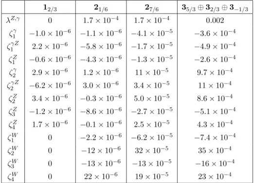
contains an exotic doublet with high hypercharge and a number of singlets. For the S_2/3, we see there are several top-like resonances, and new exotic partners charged in the SU(2)L adjoint. The pattern of anomalous gauge couplings generated by the light top partners is shown in table 2.

We see that the exotic contributions dominate over those of the SM-like resonances because of their quantum numbers. Therefore, unless the exotic resonances are heavier than the SM-like ones, they are dominant in the anomalous gauge couplings. These exotics resonances may therefore be the first manifestation of scenario with strongly interacting Higgs. If anomalous gauge couplings are indeed measured, the next step would be to identify the pattern of deviations. The first natural analysis would be to test the hypothesis of a single dominant resonance, comparing the data to the various patterns shown in table 2. On the other hand, because of the possible mass splittings, identifying the global symmmetry group using the mild dependence onN would probably be very challenging.

Overall the generic perturbative contributions described above display interesting per-spectives for the search and study of composite Higgs models in TeV precision physics, al-though the predicted deviations are small and rather high experimental precision is needed. However, although these contributions to the _L∂ Lagrangian are well under control, they might not be the only ones present. In the paradigm of a conformal strong sector sponta-neouly broken in the IR, the theory also contains a light scalar, pseudo Goldstone boson of the broken scale invariance, the so-called dilaton. The couplings of the dilaton to the rest of particles are strongly constrained by the nonlinearly realized conformal symmetry. It couples to the trace of the energy-momentum (EM) tensor of the elementary and strong sectors. The trace of the EM tensor of the massless (elementary) gauge fields vanishes classically but not at the quantum level. The dilaton couples to the large trace anomaly

7_{Other light vector-like fermions, such as τ or bottom partners, can be present in some models. Our}

results trivially generalize to these cases.

8_Notice

JHEP03(2014)102

λZ,γ 0 1.7_×10−4 _1.7×10−4 _0.002 ζ₁γ ₋1.0_×10−6 _−1.1×10−6 _−4.1×10−5 _−3.6×10−4 ζ₁γZ 2.2_×10−6 _−5.8×10−6 _−1.7×10−5 _−4.9×10−4

ζZ

1 −0.6×10−6 −4.3×10−6 −1.3×10−5 −2.6×10−4 ζ₂γ 2.9_×10−6 _1.2×10−6 _11×10−5 _9.7×10−4 ζ₂γZ ₋6.2_×10−6 _3.0×10−6 _3.4×10−5 _11×10−4

ζ₂Z 3.4_×10−6 _−0.3×10−6 _5.0×10−5 _8.6×10−4 ζ₃Z ₋1.2_×10−6 _−8.6×10−6 _−2.7×10−5 _−5.1×10−4 ζZ

4 1.7×10−6 −0.1×10−6 2.5×10−5 4.3×10−4 ζW

1 0 −2.2×10−6 −6.2×10−5 −7.4×10−4 ζ₂W 0 ₋12_×10−6 _32×10−5 _35×10−4 ζ₃W 0 ₋13_×10−6 _−13×10−5 _−16×10−4 ζ₄W 0 22_×10−6 _19×10−5 _23×10−4

Table 2. Pattern of anomalous couplings generated by the various top partners from F2/3 and

S2/3in units of Λ =mΨ. The masses of resonances on each column are potentially different.

generated by the running of the gauge coupling driven by composite states above the scale of conformal breaking, see e.g [19] and references therein.9 The tree-level exchange of a dilaton would thus generate operators of the form

FµνFµνFρσFρσ, FµνFµνZρσZρσ, FµνFµνW+ρσWρσ− (5.3)

contributing to the_L∂Lagrangian. The Lorentz structure implies that only theζ1couplings

can be modified by the dilaton, while the others remain unaltered.

To get a handle on the leading contributions from the dilaton, let us take the crucial assumption that the strongly interacting CFT has a large number of colors Nc. In that case one can invoke the qualitative version of the AdS/CFT correspondence, to describe the composite Higgs models in terms of a weakly-coupled five-dimensional theory. The KK modes of this warped extra dimension are identified as the resonances of the 4d strong sector, while the dilaton of the 4d theory is identified with the radion mode. However, in addition to describing the dilaton, a striking phenomenological prediction of the AdS5

picture is the presence of light KK gravitons near the IR brane. This implies in the 4d picture the existence of a set of composite spin-2 resonances coupling to the EM tensor of the other fields present.

We are now going to switch to the 5d picture, to compute all these effects together. Following our line of work , we will try to provide results as model-independently as possible.

9_{There are also small contributions to trace anomaly from loops of elementary fields and from a possible}

JHEP03(2014)102

6 Integrating out a warped extra-dimension

We now turn to 5d theories with a warped background. We define an effective framework including the Randall-Sundrum models as well as the pNGB composite Higgs models of section 5. The framework is described below, and details of the calculations are collected in the appendix. Let us briefly summarize the configuration of the effective framework.

• We describe the 5d background by two free parameters ˜kand κ, that are related to the curvaturek and the warp factorǫasκ=k/MP l and ˜k=ǫk respectively.

• The Higgs localization is controled by the parameterν, whereν =_∞ is an IR brane Higgs and ν= 0 corresponds to a composite pNGB Higgs.

• The radion has mass mφ, while its couplings are fixed byκ,k˜.

• Gauge fields are either on the IR brane or in the bulk. If they are in the bulk, the gauge group is either the SM or extended in the custodial and/or gauge-Higgs unification models.

• In the bulk gauge fields case, SU(2)L and U(1)Y IR brane kinetic terms (BKTs) respectively parametrized asr,r′ _{are present.}

6.1 The 5d framework

The spacetime metric of theories with a warped extra dimension can be written in general as

ds2=γM NdxNdxM =a(z)−2(ηµνdxµdxν−dz2), (6.1)

withηµν =diag(1,−1,−1,−1),z∈[zU V, zIR]. The action reads

S =₋ Z

dx5√₋g_{M3(_R+ Λ) + 1 4FM NF

M N

−DMH†DMH− i 2ΨΓ¯

M←→_D MΨ

+m2_H|H_|2+mΨΨΨ +¯ B}.

(6.2)

Here M is the 5d Planck mass, _R is the Ricci scalar and Λ is a negative cosmological constant. _Bcontains the boundary terms, and m2

H and mΨ denote the 5d masses

respon-sible for the localization of the Higgs and fermion zero modes. For the purpose of deriving the low-energy effective Lagrangian, there is in general no need to specify a particular background, many analytic expressions can be derived in terms ofa(z) and zero mode pro-files [20]. Any stabilization mechanism will induce such a nontrivial metric, we will work under the approximation that such backreaction is neglected.

The AdS5 metric a(z) =kz then follows from eq. (6.2) with Λ = 12k2. The quantity k is the inverse curvature radius, we take the location of the UV boundary to be z0 =

1/k without loss of generality and define ˜k _≡ 1/z1 where z1 is the location of the IR

boundary. The 4d reduced Planck mass is related to the scaleM asM3 _=kM2

P l. TheAdS5 background can be described in terms of two parameters, for our purpose it is appropriate to choose the IR scale ˜kand the dimensionless quantity

JHEP03(2014)102

requiring higher curvature terms _R5/M∗2 to be smaller than 1. Here R5 = 20k2 is the

size of the AdS curvature and M∗ is seen as the cutoff of the 5d theory, estimated by naive dimensional analysis [21,22], to beM∗3≈(24π3)MP l2 k. Note that the narrow-width approximation breaks down for κ & 2 (κ & 0.3) for the case of bulk (IR brane) localized SM fields [22,23]. This will not constitute a problem for integrating out KK gravitons, as for this purpose one goes in the zero momentum limit for which the imaginary part of the self-energy vanishes.

Finally, we include the IR brane kinetic terms

B ⊃δ(z₋z1) rI

4F I

µνFI µν. (6.4)

These BKTs are generically present in the theory, and are radiatively generated even if they are set to zero at a given scale. These BKTs induce various effects which turn out to be crucial for the phenomenology of the bulk gauge scenario, in particular they distort the gauge KK spectrum. The physical gauge coupling is given by10

(gI)2= (g I

5)2

V +rI₁ . (6.5)

Equation (6.5) constrainsrI _>−V.

The first KK modes have a mass related to the IR scale ˜k by _O(1) factors. The first graviton and gauge modes without BKTs have a mass

m2 ≈3.8 ˜k , m1 ≈2.4 ˜k . (6.6)

The first KK gauge modes in presence of respectively positive and negative BKTs _|rI|>

O(1) have a mass11

m1≈

√ 2

r rI +V

rIV ˜

k , m1≈3.9 ˜k . (6.7)

The first KK fermions with flat profile have a mass m1/2 ≈2.4 ˜k. However, fermions with mixed Neumann-Dirichlet boundary conditions and the appropriate sign of bulk mass can become exponentially light with respect to ˜k. It is important to keep this possibility in mind as it can have consequences for the size of the anomalous gauge couplings. This constitutes the 5d version of the light top partners of the composite Higgs setup. The other quantities commonly used in the AdS5 background are the warp factorǫ≡˜k/k and

the volume factor V = logk/k˜. Notice that in order to solve the hierarchy problem, i.e. ˜

k_≈1 TeV, one needsV _≈37. Defining ν=

q

m2_H/k2_{+ 4, the Higgs profile along the fifth dimension is}

fh(z)∝z2+ν. (6.8)

10_{We restrict to IR BKTs. In presence of UV BKTs, the physical gauge coupling becomes (g}I₎2 ₌

(gI5)2/(V +rI0+rI1). 11_Forr

JHEP03(2014)102

described by a boundary 4d Lagrangian_{L ⊃} δ(z₋z1)L4Hd. The lower bounds isν = 0,12 for this value the Higgs field is in the bulk, but is still localized towards the IR brane.

The case ν = 0 also describes the couplings of a possible zero mode of the fifth com-ponent of a gauge field,A5. Other properties of aA5 like the 5d energy-momentum tensor

are different from those of a fundamental scalar. However, for our purpose, only the tree-level profile matters. We can therefore interpret our ν = 0 fundamental Higgs as an A5.

Identifying the Higgs as a A5 is the central idea of gauge-Higgs unification models. In

the holographic picture, it corresponds to the Goldstone boson of the global symmetry spontaneously broken by the strong dynamics. The ν = 0 case corresponds therefore to a holographic description of the composite pNGB models that we discussed in section 5.

The radion in a slice of pure AdS is massless. In the holographic picture it corresponds to the dilaton, i.e. the Goldstone boson of scale invariance spontaneously broken by the strong dynamics. Once the size of the extra-dimension is fixed by a stabilization mechanism, the AdS background gets deformed and the radion obtains a mass. In the holographic picture this corresponds to an explicit deformation of the CFT by a relevant operator. In many classes of models the radion is lighter than the IR scale, mφ ≪ k˜. In this limit its profile stays unperturbed to leading order, its couplings are given by those of a massless radion up to corrections of_O(m2_φ/˜k2), and the only free parameter is its massmφ.

Contrary to scalar fields, gauge fields cannot be continuously localized from bulk to brane. We consider two separate cases, with gauge fields propagating in the bulk and on the IR brane respectively. The case of bulk gauge fields corresponds to a global symmetry of the CFT, and one can extend the bulk gauge group to a larger symmetry including in particular the custodial SU(2)R, as motivated by electroweak precision observables (see section 7). We will consider both the non-custodial and custodial cases.

Hereafter we derive the effective 4d Lagrangian arising from this 5d framework. We are going to integrate out the radion and KK excitations of gauge, fermions, and gravity. The effective 4d action resulting from integrating out gravity in a slice of AdS5 has been

computed in ref. [15] and is reviewed in appendixB. The SM fields couple to 5d gravity via the modified 5d energy-momentum tensor ¯TM Ndefined in eq. (B.7). The piece proportional to ( ¯Tµν)2 reads

Leff =

1 4M3

Z z₁

z0

dz (kz)3 [Θµν(z)−Ω−2(z) Θµν(z1)]2 (6.9)

where Θµν is the ¯Tµν integrated over the 5th dimension (see eq. (B.8)) and Ωp is defined as

Ωp =

zp₋z₀p

z₁p₋z₀p. (6.10)

The leading contribution proportional to ( ¯T55)2 comes from the radion. Its Lagrangian

reads

Lφ= 1 2(∂µφ)

2

−1₂m2_φφ2+ r

2 3

ǫ MP l

Θ(x, z1)φ (6.11)

12_{This corresponds tom}2

JHEP03(2014)102

eq. (B.12) for an explicit expression. Integrating outφleads to

Leff = ǫ2

3M2

P l 1 m2

φ

[Θ(x, z1)]2 . (6.12)

Integrating out the tree-level KK gauge fields leads to an effective action

Leff =−

(gI₅)2

2 a

I

XY JXI µ JY µI (6.13)

where X, Y = H, f label the Higgs and fermions zero modes and I labels the 5d gauge field. TheJ_XI µ are the zero mode currents. The quantitiesaXY are given by

aI_XY = Z

dz kz (ΩX−ΩI) (ΩY −ΩI) (6.14)

where13

ΩI =

    

   

log(kz) V +rI

1

(++ gauge field)

0 (+₋ gauge field)

1 (₋+ gauge field)

(6.15)

We are only interested in the oblique and flavor diagonal part of the effective action and therefore can set universally Ωf = 1 as if all fermions were exactly UV localized.14 The integrated profile of the Higgs is given by ΩH = Ω2(ν+1). Details of the calculations are

left for appendix Band can be found in [15,20].

Finally, the loops of KK modes are already included in the general formulas of section4. The only work to do is to sum the contributions over the tower of KK modes. This translates to small enhancement factors, as the operators we consider are UV-finite, and thus dominated by the lightest KK modes. The enhancement factors for the inverse-quartic sum are rather close to one. The zeroes of the Bessel functions Jρsatisfy [24]

X

n 1 (mρ,n)4

= 1

(2˜k)4_{(ρ+ 1)}2_{(ρ+ 2)} (6.16)

For instance, for a KK gauge mode with J0(m1/k˜) = 0 one has to make the replacement

1 (2.405)4 ≈

1 33.5 →

1

32 (6.17)

i.e., a correction factorK_ρ(4)_=0≈1.045. The correction increases with ρ, e.g. K_ρ(4)_{=1 ≈}1.123. The correction are larger for the inverse-square sum, entering in the computation of _OW3,

X

n 1 (mρ,n)2

= 1

(2˜k)2_{(ρ+ 1)} (6.18)

e.g.K_ρ(2)₌₀ = 1.45 and K_ρ(2)₌₁= 1.83.

13_{In presence of both UV an IR BKTs, Ω}

I=log(kz)+r I 0 V+rI

0+r I 1

for ++ gauge fields.

14_{Deviations from UV localization lead to non-oblique operators for heavy fermions, such as anomalous}

JHEP03(2014)102

Here we derive the contributions to the effective Lagrangian from KK-gravitons and from the radion. We distinguish two separate cases depending whether gauge fields are confined on the IR brane or propagate in the bulk. For simplicity, a common BKT has been assumed, rI =r. Note in the numerical results in sections7 and 8 we keep the dependence on both

r and r′_.

For gauge fields in the bulk, the KK gravitons contribute as

L(8) ⊃ κ

2

128 ˜k4

1 + 4r+ 8r2

(r+V)2

−1

4(O8+O9+ 2O11) +O13+O14+ 2O16

+ κ

2

64 ˜k4

1 r+V

(1 +ν)(5 +ν+ 4r(3 +ν)) (3 +ν)2

−4_O3−4O4+O6+O7

.

(6.19)

Integrating out the radion leads to

L(8) ⊃ κ

2

192 ˜k2

1 (V +r)2

1 m2

φ

(_O8+O9+ 2O11). (6.20)

The radion also contribute to operators of_L(6),

L(6)⊃ κ

2

12 ˜k2

1 V +r

m2

h

m2

φ

OW W +OBB+OGG

, (6.21)

where mh is the physical Higgs mass. This contribution can be see as a manifestation of Higgs-radion mixing in the range mh < mφ<k˜. KK gravitons do not contribute to these operators as their contribution is proportional to the trace of the gauge EM tensor and thus exactly zero.

We finally remark that there is a contribution to the operator _OD2 from 5d gravity. This has been computed in a model of 5d supergravity coupled to matter fields in ref. [15], here we simply take the result from there by omitting the contributions from superpartners. One finds

L(6)⊃ − κ

2

6 ˜k2

(1 +ν)2

3 + 2ν OD2 (6.22)

As already noticed in ref. [15], this result diverges in the localization limit ν _{→ ∞}. The reason for this is that 5d gravity couples to 5d mass terms, and hence perturbation theory breaks down for large (but in principle finite) ν. However, starting directly from brane-localized fields (without taking the limit ν _{→ ∞}) one can show that these contributions are exactly zero.

For gauge and matter fields on the IR brane, one can simply take the limit r, ν _{→ ∞} in eqs. (6.19), (6.20) and (6.21), leading to

L(8) ⊃ κ

2

16 ˜k4

−1

4(O8+O9+ 2O11) +O13+O14+ 2O16

+ κ

2

16 ˜k4

−4(_O3+O4) +O6+O7

.

(6.23)

JHEP03(2014)102

Let us define the functions of the Higgs bulk mass

f1(ν) =

2(1 +ν)2

(2ν+ 3)(ν+ 2), f2(ν) =

(1 +ν)(3 +ν)

(2 +ν)2 . (6.24)

For a brane Higgs, their values are f1(∞) = f2(∞) = 1. For a pseudo-Goldstone Higgs, f1(0) = 1/3, f2(0) = 3/4. We do not display explicitely the r-dependent terms, nor

contributions that are subleading in 1/V. Both can be easily obtained from our general expressions. In the non-custodial case, one obtains

L(6)⊃ − 3g

2_+g′2

8˜k2 V f1(ν)OD2 + g2

4˜k2f2(ν)OD− g2 ˜ k2

1 8VO4f

− g ′2

4˜k2V f1(ν)O

′ D2+

g′2

4˜k2f2(ν)O

′ D −

g′2

˜ k2

1 8VO

′

4f.

(6.25)

In the custodial case,15 _{we get}

L(6)⊃ −3g

2_{+ 3g}′2

8˜k2 V f1(ν)OD2 + g2

4˜k2f2(ν)OD− g2

˜ k2

1 8VO4f

+ g ′2

4˜k2f2(ν)O

′ D2 +

g′2

4˜k2f2(ν)O

′ D−

g′2

˜ k2

1 8VO

′

4f.

(6.26)

6.4 Contributions from KK-loops

From the KK Higgs, we find16

L(6)⊃ − g

2

16π2

1 288

K0(2)

m2 0

OW3, (6.27)

L(8)⊃ g

4

16π2 K0(4)

4m4 0

33_O9+ 2O10+ 8O14+ 20O15

20160

+g

2_g′2

16π2 K0(4)

4m4 0

1

576(2O11+ 4O12) + 1

720(4O16+ 2O17)

(6.28)

+ g ′4

16π2 K0(4)

4m4 0

1 576O8+

1 720O13

,

wherem0 is the lightest KK Higgs mass and the correction from the KK tower amounts to

a very mild enhancement factorK0(4). As already stated, contributions of spin-zero states

are suppressed compared to those of nonzero spin. The Higgs KK tower thus plays no role and we will neglect it in what follows. From the KK SM-like fermions, we find

L(6)⊃ g

2

16π2

1 12

K₁(2)_/2

m2

1/2

OW3, (6.29)

15_{The custodialO}

D2 also gets a subleading coefficient−g

′2

8˜k2f2(ν).

JHEP03(2014)102

L(8) ⊃ g

4

16π2 K₁(4)_/

2 m4

1/2

−3_O9−32O10+ 40O14+ 58O15

840

+g

2_g′2

16π2 K₁(4)_/2

m4_1/2

−₃₆1 (_O11+ 2O12) +

7

90(2O16+O17)

+ g ′4

16π2

95 18

K₁(4)_/ 2 m4

1/2

−₃₆1 O8+

7 90O13

.

(6.30)

From the KK SM-like vectors without custodial symmetry, we find

L(6) ⊃ − g

2

16π2

1 48

K1(2)

m21

OW3, (6.31)

L(8) ⊃ g

4

16π2 K1(4)

m4 1

−69_O9−106O10+ 528O14+ 228O15

1120

(6.32)

Finally, in presence of custodial symmetry, an additional operator

L(8) ⊃ g ′4

16π2 K1(4)

m41

−₃₂5 O8+

27 40O13

(6.33)

is generated. Here, the enhancement factors that take into account the tower of KK resonances are approximately given by K(n) _≈K(n)

ρ=0 for both fermions and vectors. They

are thus approximately given by K(2)_≈1.45 and K(4)_≈1.045.

7 Bounds from Higgs and electroweak precision measurements

Let us derive the bounds imposed by electroweak and Higgs precision physics. The expected deviations to theS and T parameters [25,26] and to Higgs anomalous couplings in terms of the effective operators of_L(6) _{are [9]}

S =

2swcwαW B +s2w(αD−2α4f) +c2w(α′D−2α′4f)

v2

Λ2 ,

T =

−1₂α′_D2 +

1 2α ′ D− 1 2α ′ 4f v2

Λ2, (7.1)

aZ = 1 +

1 2αD2−

1

4(αD −α4f) + 1 4α ′ D2 v2 Λ2 ,

aW = 1 +

1 2αD2−

1

4(αD −α4f)− 1 4α ′ D2 v2

Λ2 , (7.2)

with

LhVV =aZ

m2

Z

v h(Zµ) 2_+a

W 2m2

W

v h(Wµ)

JHEP03(2014)102

propagators. It turns out that for the bulk gauge scenario, the exact predictions for theS, T parameters are

S = 2π f2(ν)

1 + (r+r′)2 +ν 3 +ν

v2

˜

k2 , (7.4)

T = π V 2c2

w

f1(ν)

1 +r ′

V

v2

˜

k2 , (7.5)

and T = 0 exactly in the custodial case.17 These surprisingly simple expressions are the result of exact cancellations among more complicated contributions from the various operators. In particular no such simple expressions can be obtained for the aV or the

κi. One might also check that for the case of a pNGB Higgs, ν = 0, and for r = r′ the expression for S coincides precisely with the one obtained in ref. [28]. Finally, for brane gauge fields, contributions only come at the loop level and are thus much smaller, so that we do not consider them.

The KK gauge fields also induce Higgs anomalous couplings. We do not display the full expressions including BKTs, as they are rather lengthy. For vanishing rI one gets in the non-custodial case

aZ ≈1−

3g2_{+ 2g}′2

16 V f1(ν) v2

˜

k2 aW ≈1−

3g2

16 V f1(ν) v2

˜

k2 . (7.6)

In the custodial case one gets18

aZ ≈aW ≈1−3g

2_{+ 3g}′2

16 V f1(ν) v2 ˜

k2 . (7.7)

In both cases, the aW −aZ discrepancy is proportional to g′2. Once including the BKTs, it turns out that in both cases aW −aZ grows large for negative values of r′ and goes to zero for positive values of r′_{. For brane gauge fields, these contributions are zero. Finally} the radion also generates the new tensorial Higgs couplings

Lhγγ =ζγh(Fµν)2, (7.8)

with

ζγ =

κ2 12

s2_w r+V +

c2_w r′_+V

m2

hv

m2

φk˜2

. (7.9)

17_{In presence of light exotic fermions there can be important contributions to S and T from loop}

ef-fects [27]. These can be interpreted as arising from operator mixing when performing the RG evolution between the UV and EW scales.

18_{An important subtlety is that the equalitya}

JHEP03(2014)102

S= 0.05_±0.09, T = 0.08_±0.07 (7.10)

with a correlation coefficient of +0.91. Constraints on aV (for aW = aZ) and the ζi are taken from the global fit of [9]. At 95% CL one has

0.96< aV <1.21, −6.1< ζγv×103<0.9, (7.11)

the constraints on otherζi being less stringent for our purpose.

These constraints translate as the following 95% CL bounds on the KK modes and parameters. Consider first vanishing BKTs. From theS, T parameters in the non-custodial case, we obtain19

m1|_ν=∞>14.7 TeV, m1|_ν=0 >8.1 TeV. (7.12)

In the custodial case,

m1|_ν=∞>7.7 TeV, m1|_ν=0 >6.6 TeV. (7.13)

From theaV bounds we have

m1|_ν=∞>5.8 TeV m1|_ν=0 >3.4 TeV (7.14)

in the custodial case. Although the aV bound is not available in the non-custodial case, similar numbers are expected. In case of a bulk Higgs with ν = 0, there is therefore no longer a strong motivation to introduce custodial symmetry, as the improvement in the bounds is only marginal. From ζγ we also obtain a relatively weak bound on the radion mass,

˜

k mφ> κ(221 GeV)2. (7.15)

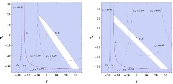
Interestingly, the above bounds get relaxed in presence of BKTs.20 The brane and pNGB Higgs cases are similar, we focus on the pNGB Higgs case which is slightly favored. In both custodial and non-custodial cases a region appears where the contributions toS, T are significantly reduced. The allowed 95% CL regions in the plane (r, r′_{) for ˜k= 3 TeV} are shown in figure 1. We use the aV constraint when aW ≈ aZ. We also show (dashed lines) how this constraint would apply to aW, aZ separately. It appears that the current constraint on aV, although already stringent for aV <1, is still subleading on most of the parameter space. We also extrapolate how this limit would evolve for aW,Z >0.99 instead ofaV >0.96. It turns out that such bound would be clearly competitive with respect to the

S, T parameters. Finally, it is interesting to notice that the favored regions either feature light KK Wµ or a light KKBµ, with mass m1≈0.24 ˜kfor respectivelyr >0 andr′ >0.

Here we do not discuss in detail the limits from direct LHC searches as they are, by the time of this paper, weaker than the indirect bounds derived above. The most stringent

19_{Slightly more optimistic numbers have been obtained recently in ref. [30] for the case of a brane localized}

Higgs. Note however that these authors quote 99% CL bounds on ˜kand used an older (pre Higgs-discovery) fit for theS, T ellipse.

JHEP03(2014)102

Figure 1. Electroweak, Higgs and gauge precision bounds for ˜k= 3 TeV. The regions excluded at 95% CL are shown in blue, the allowed regions are shown in white. TheS, T limit is shown in dark, theaV limit is shown in dark blue and in dashed lines when aW 6=aZ, and theκ3 limit is shown in purple. Are also displayed extrapolated limits from more stringent constraints aW,Z > 0.99,

|κ3|<0.01. The red point denotes the case of vanishing brane kinetic terms. Left and right panels respectively correspond to non-custodial and custodial cases for a pNGB Higgs (ν= 0).

current limits result from KK gluons decaying to top pairs, yielding m1 > 2 TeV [38].

Bounds on KK gravitons are much weaker, with m2 >850 GeV (at κ= 1.0) for the bulk

SM case [39] and m2 >1 TeV (at κ = 0.1) for the IR-brane SM case [40]. Direct searches

are further disfavored at large κ as the KK gravitons are not narrow resonances anymore, while no such problem affects the effective operators. A recent study of the discovery potential at the LHC can be found in [41]. We remark that the new indirect bounds for vanishing BKTs derived above most likely push the KK resonances beyond the reach of the LHC, unless some mechanism suppresses the coupling of the Higgs field to electroweak KK modes, for instance by modifying the geometry in the IR [33–35], reducing in particular theT parameter in non-custodial models [20,36,37]. Another precision observable we do not consider here in detail is the measurement of theZb¯bvertex. This quantity is sensitive to the details of the model, including the realization of the custodial sector.21

8 Probing a warped extra dimension using anomalous gauge couplings

We now consider the anomalous gauge couplings generated from our effective warped extra dimension framework. In a first part we discuss the case of vanishing BKTs. The effect of sizeable BKTs will be discussed afterwards. The leading contributions are summarized in table 3, we now discuss in details its content.

For vanishing BKTs, the contributions from the KK gravitons depend only on the background (here AdS) and on the location of gauge fields. They are enhanced by about

21_{Bounds comparable to the ones from the oblique parameters (i.e.m1∼4−6 TeV) can be achieved by}

JHEP03(2014)102

Coupling Bulk gauge fields IR gauge fields

Non-custodial Custodial

αD/Λ2 {0.62,0.46}/m21 {0.62,0.46}/m21 ∼0

α′

D2/Λ2 {−6.8,−2.3}/m21 {0.19,0.14}/m21 ∼0

κ1 ∼0 ∼0 ∼0

κ2,3,4 {2.88,0.84}v2/m21 {−0.38,0.28}v2/m21 ∼0

κ5 {2.22,0.65}v2/m21 {−0.29,−0.22}v2/m21 ∼0

λZ,γ (6.8/m21/2−1.7/m

2

1)×10−4 ∼0

η1W {−0.35,−0.20}κ2m2W/m42 −52κ2m2_W/m42

ηW

2 {0.088,0.049}κ2m2W/m42 13κ2m2W/m42

ηZ

1 {−0.18,−0.098}κ2m2Z/m42 −26κ2m2Z/m42

η2Z {0.044,0.025}κ2m2Z/m42 6.5κ2m2_Z/m42

ζ₁γ (0.04κ2_/(˜k2_m2

φ)−0.2/m41/2−0.1/m

4

1−3.0κ2/m42)×10−4 −3.3κ2/m42

ζ1γZ (0.06/m41/2−0.08/m

4

1)×10−4 ∼0

ζ1Z (0.08κ2/(˜k2m2φ)−0.07/m41/2−0.7/m

4

1−6.0κ2/m42)×10−4 −6.5κ2/m42

ζW

1 (0.15κ2/(˜k2m2φ)−0.2/m41/2−0.7/m

4

1−1.5κ2/m42)×10−4 −13κ2/m42

ζ2γ (0.4/m41/2+ 0.47/m

4

1+ 12κ2/m42)×10−4 13κ2/m42

ζ₂γZ (0.4/m41/2+ 2.4/m

4

1)×10−4 ∼0

ζZ

2 (1.4/m41/2+ 4.4/m

4

1+ 24κ2/m42)×10−4 26κ2/m42

ζZ

3 (−0.14/m41/2−1.5/m

4

1)×10−4 ∼0

ζ4Z (0.7/m41/2+ 2.1/m

4

1)×10−4 ∼0

ζW

2 (1.5/m41/2+ 5.7/m

4

1+ 48κ2/m42)×10−4 52κ2/m42

ζW

3 (−0.3/m41/2−1.1/m

4

1)×10−4 ∼0

ζ4W 1.3/m41/2×10

−4

∼0

Table 3. Pattern of the leading anomalous gauge couplings induced by an AdS5 background with vanishing brane kinetic terms, depending on gauge fields location and on the presence of custodial symmetry. The first KK modes are all related to the KK scale ˜k. The first KK gauge field has m₁ = 2.4 ˜k, the first KK graviton has m₂ = 3.8 ˜k. The first SM-like fermion KK mode hasm1_/

2= 2.4 ˜kif flat or is heavier otherwise. The radion massmφ ≪k˜ is a free parameter. The

JHEP03(2014)102

occur only in the bulk gauge scenario because brane localized gauge fields do not couple to the radion at tree level. The contributions from KK gauge fields, KK Higgs, KK fermions only occur in the bulk gauge scenario as these modes are absent in the brane gauge sce-nario. The KK gauge contributions depend on custodial symmetry. Finally, the KK Higgs contributions are always negligible with respect to loops of other spin. We only show SM-like KK fermion contributions in table 3. They are slightly smaller than the ones from KK gauge fields. Certain fermion KK modes with Neumann-Dirichlet boundary conditions can have a mass m1_/2 ≪k˜, which would enhance significantly their contribution. This is

precisely how the light exotic resonances of composite Higgs models of section5appear in the 5d dual description. Their contributions can be added with the help of table 2.

Let us discuss the relative size of the contributions to the HDOs. Consider first the L(6) Lagrangian. For bulk gauge fields, the _OD2 and O′

D2 contributions are the largest

ones in the non-custodial scenario as they are enhanced by a volume factorV. _O′

D2 is not

enhanced by V in the custodial case (and will actually cancel with _O′

D, O′4f within the

T parameter). The _O4f contribution is suppressed by V and is always subleading. The OD2 does not feed into anomalous gauge couplings but is relevant for Higgs couplings,

as discussed in the previous section. All _OF F operators can only be loop-generated from renormalizable couplings. However _OW W and OBB do receive tree-level contributions from gravity. These two operators do not contribute to anomalous gauge couplings, but modify Higgs couplings, as discussed in the above section. In contrast, the_OW B operator contributes to anomalous gauge couplings, but does not receive contributions from gravity. As other large contributions are present, we take the computation of _OW B to be beyond the scope of our study, and we choose to neglect it. The dominant contributions to _Lv_CGC Lagrangian are therefore_OD′ 2 in the non custodial andOD,O

′

D2 in the custodial case. For

the_L∂

CGC Lagrangian, contributions arise only from KK SU(2)Lfermions and KKW loops.

Let us turn to the _L(8) Lagrangian. Contributions to _Lv_NGC come only from KK gravitons. For _L∂, both KK gravity and KK matter contribute. The radion contribution is small. In the broken phase, it contributes only to the ζ1 couplings, because it couples

only to the trace of energy-momentum tensors. It turns out that tree-level TeV gravity and loop-level EW processes can be of the same order of magnitude depending onκ2_{. Moreover}

fermion contributions can be large if one of the KK fermion gets light. It is thus necessary to keep all the contributions. It is worth noticing that the contribution from the KK gauge loop to_O14is larger by almost one order of magnitude with respect to the ones of the other

HDOs. The contributions discussed above will dominate the anomalous couplings and are thus the ones that can be probed in the first place.

Let us now adopt the point of view of anomalous couplings. We first discuss _LCGC.

The charged anomalous gauge couplingsκ2...5 probe the existence of KK gauge modes. In

JHEP03(2014)102

LKK gauge modes and of KK fermions. Although they are loop-generated and thus smaller than the κ2...5, one expects the deviation induced by the λZ,γ to compete with the κ2...5 in the v < E < Λ regime. A naive estimate suggests that the effect of these operators in the total cross-section becomes dominant for E _≈4πv _≈3 TeV. However as the effects of this effective coupling grow with the energy, it may be more appropriate to look for deviations in the high-pT tails of kinematic distributions. The search for these anomalous couplings is particularly appropriate at LHC, which is typically exploring the regimev < E <Λ.

The ηW

1,2 coupling are sensitive to KK gravitons. Measuring these couplings seems

challenging in ATLAS and CMS because of the SM background. On the other hand FP detectors like the ones foreseen for the LHC upgrade may help probe these couplings with a smaller background using proton tagging. The σ(γγ_→ W W) cross-section is enhanced in presence of these couplings [43,44].

Let us turn to_LNGC. In this work we focus on two-photon neutral couplings as they are

forbidden in the SM at tree-level. The rare processes induced by the anomalous couplings may be probed with high precision using the AFP detector. The η₁Z_,2 are probing KK gravitons. Contrary to ηW

1,2, there is no tree-level SM background. They may have a good

potential both at ATLAS/CMS and using FP detectors. The ζ1 operators receive various

contributions from gravity and matter in case of bulk gauge fields, and are rather small. We limit ourselves to a heavy radion, out of reach from direct detection, in order to keep the EFT valid. Its contribution turns out to be small with respect to gravitons. In case of brane gauge fields, the ζ1,2’s are larger and sensitive to the KK gravitons, while the ζ3,4’s

are vanishing.

Overall, the states likely to be discovered by the measurement of anomalous gauge couplings are the KK gauge fields if gauge fields are in the bulk, and the KK gravitons if gauge field are brane-localized. Fermion contributions are somewhat smaller, although they could be enhanced in presence of light KK fermions such as those present in the pNGB Higgs scenarios. Assuming similar sensitivity for η₁Z,W_,2 and the ζi’s, the latter might be favored as the LHC typically explores the v < E <Λ regime.

Let us now consider the case of sizeable BKTs. These BKTs modify the contribution to theκ2...5 couplings because of the distortion of the gauge propagator. They also modify

the gravity contributions to ηi and ζi as gravitons can couple to both bulk and brane components. We focus on the pNGB Higgs case. The LEP constraint onκ3(≈κ2) becomes

relevant, the 95% CL interval translates as

0.054< κ3 <0.021, (8.1)

and the limits are displayed on figure1. Theκ3 bound from LEP, subleading for vanishing

BKTs, becomes relevant for large negative r, r′_{. In both cases, the a}