www.hydrol-earth-syst-sci.net/15/1515/2011/ doi:10.5194/hess-15-1515-2011
© Author(s) 2011. CC Attribution 3.0 License.
Earth System
Sciences
Geostatistical radar-raingauge combination with nonparametric
correlograms: methodological considerations and application in
Switzerland
R. Schiemann1,*, R. Erdin1, M. Willi1, C. Frei1, M. Berenguer2, and D. Sempere-Torres2
1Federal Office of Meteorology and Climatology MeteoSwiss, Kraehbuehlstrasse 58, P.O. Box 514, 8044 Zurich, Switzerland 2Centre de Recerca Aplicada en Hidrometeorologia (CRAHI), Universitat Polit`ecnica de Catalunya, C/ Gran Capit`a, 2-4, Edifici NEXUS 102-106, 08034 Barcelona, Spain
*now at: National Centre for Atmospheric Science (NCAS) Climate, Department of Meteorology, University of Reading, Earley Gate, P.O. Box 243, Reading, RG6 6BB, UK
Received: 24 August 2010 – Published in Hydrol. Earth Syst. Sci. Discuss.: 16 September 2010 Revised: 16 December 2010 – Accepted: 2 May 2011 – Published: 19 May 2011
Abstract. Modelling spatial covariance is an essential part
of all geostatistical methods. Traditionally, parametric semi-variogram models are fit from available data. More recently, it has been suggested to use nonparametric correlograms ob-tained from spatially complete data fields. Here, both estima-tion techniques are compared. Nonparametric correlograms are shown to have a substantial negative bias. Nonetheless, when combined with the sample variance of the spatial field under consideration, they yield an estimate of the semivar-iogram that is unbiased for small lag distances. This jus-tifies the use of this estimation technique in geostatistical applications.
Various formulations of geostatistical combination (Krig-ing) methods are used here for the construction of hourly pre-cipitation grids for Switzerland based on data from a sparse realtime network of raingauges and from a spatially complete radar composite. Two variants of Ordinary Kriging (OK) are used to interpolate the sparse gauge observations. In both OK variants, the radar data are only used to determine the semi-variogram model. One variant relies on a traditional paramet-ric semivariogram estimate, whereas the other variant uses the nonparametric correlogram. The variants are tested for three cases and the impact of the semivariogram model on the Kriging prediction is illustrated. For the three test cases, the method using nonparametric correlograms performs equally well or better than the traditional method, and at the same time offers great practical advantages.
Correspondence to:R. Schiemann ([email protected])
Furthermore, two variants of Kriging with external drift (KED) are tested, both of which use the radar data to esti-mate nonparametric correlograms, and as the external drift variable. The first KED variant has been used previously for geostatistical radar-raingauge merging in Catalonia (Spain). The second variant is newly proposed here and is an exten-sion of the first. Both variants are evaluated for the three test cases as well as an extended evaluation period. It is found that both methods yield merged fields of better quality than the original radar field or fields obtained by OK of gauge data. The newly suggested KED formulation is shown to be beneficial, in particular in mountainous regions where the quality of the Swiss radar composite is comparatively low.
An analysis of the Kriging variances shows that none of the methods tested here provides a satisfactory uncertainty estimate. A suitable variable transformation is expected to improve this.
1 Introduction
strengths and compensating for the weaknesses of the two measurement platforms. A number of such methods exist and have been categorized by Erdin (2009) into (i) simple ad-justment techniques often used in postprocessing radar mea-surements (e.g., Gjertsen et al., 2004; Germann et al., 2006), (ii) the disaggregation of gauge fields by radar information (e.g., DeGaetano and Wilks, 2009; W¨uest et al., 2009), and (iii) geostatistical combination methods (Seo et al., 1990; Seo, 1998; Todini, 2001; Sinclair and Pegram, 2005; Haber-landt, 2007; Erdin, 2009; Velasco-Forero et al., 2009). Geo-statistical methods enjoy particular popularity and appear to outperform simpler merging techniques (e.g., Goudenhoofdt and Delobbe, 2009).
Even within the area of geostatistical methods, a wide range of choices have to be made when planning for a par-ticular application. These choices regard, for example, the actual combination method (e.g., kriging with external drift, cokriging), the kriging neighbourhood (global vs. local), the technique used to estimate the parameters of the geostatis-tical model (e.g. least-squares, maximum-likelihood estima-tion), and the transformation of the precipitation variable. In addition to these issues, there are several options for mod-elling spatial dependencies in the precipitation data. Correl-ograms (or semivariCorrel-ograms) used for kriging are customar-ily one-dimensional, but two- or higher-dimensional corre-lation maps are also used and are one way of taking spatial anisotropy into account. Furthermore, correlogram models can be parametric or nonparametric, they can be obtained from the radar or the raingauge data, and they can be esti-mated flexibly on a case-by-case basis or with data from a longer period of time.
Recently, nonparametric correlograms based on spatially complete radar rainfall fields have been used in combining radar and raingauge data (Cassiraga et al., 2004; Velasco-Forero et al., 2009). The estimation of nonparametric correl-ograms is fast and robust (in particular, no parametric model has to be fit) and anisotropy is naturally taken into account. The objective of this study is to compare the estimation of nonparametric correlograms with the traditional estimation of semivariograms, and to test their application in the geo-statistical combination of hourly raingauge and radar data in Switzerland. Additionally, the present application tests in how far geostatisitical methods that traditionally rely, implic-itly or explicimplic-itly, on a Gaussian data model, can be applied to highly non-Gaussian and non-continuous hourly precipi-tation data in complex terrain. This paper describes one of several current activities in the MeteoSwiss project Combi-Precip, which aims at the operational provision of spatial pre-cipitation estimates for Switzerland on the subdaily timescale based on the combination of radar and raingauge measure-ments.
The structure of this paper is as follows: Sect. 2 introduces the study domain and data, compares the modeling of spatial dependence with the nonparametric correlogram and tradi-tional parametric semivariograms, presents the geostatistical
combination (Kriging) techniques tested here, and how the quality of both the estimated precipitation fields and the es-timated uncertainty in these fields is evaluated. Thereafter, Sect. 3 presents several examples and a systematic evalua-tion of the combinaevalua-tion methods. Secevalua-tion 4 concludes this study.
2 Methods and data
2.1 Study area and data
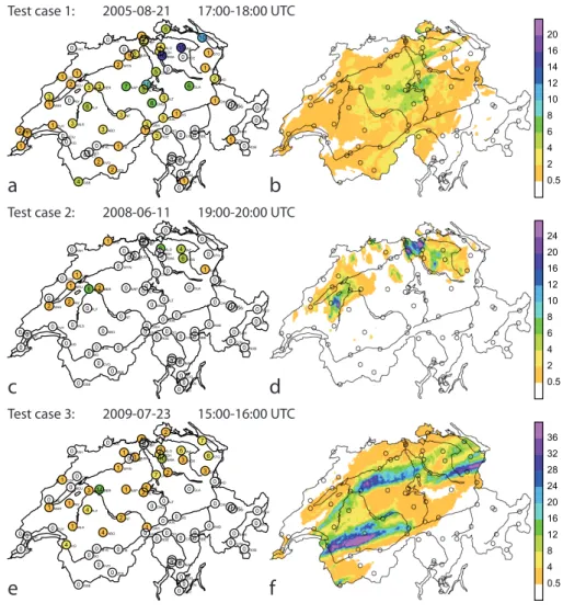
The study area is Switzerland and has a surface area of 41 285 km2. We combine raingauge and radar data on the hourly timescale. On this timescale, data from 75 automatic raingauges of the SwissMetNet (SMN) are available. These gauges provide measurements at 10-minute intervals in real time. They are fairly homogeneously distributed throughout the country, but remote areas and high elevations are some-what underrepresented. The gauge locations are indicated in Fig. 5.
Radar data are taken from a composite of three Me-teoSwiss radars (see Germann et al., 2006, Fig. 1, for the radar locations). The composite is available at 5-min inter-vals as a gridded field of 1 km resolution covering Switzer-land and adjacent areas. The construction of the radar com-posite is discussed in Germann et al. (2006). In particular, the radar precipitation field is adjusted to gauge measurements using a single factor for each of the three contributing radars. The factor is determined from radar-gauge agreement after integration over a large time window (6 months) and several gauges in the vicinity of the radar. This is a “climatological” bias correction; it involves a small subset of the gauge net-work considered in this study, and does not correct for the substantial biases that can occur in the radar composite on the hourly timescale. Further details concerning the charac-teristics of the two measurement platforms and uncertanties can be found in Sevruk (1985); Frei et al. (2006); Germann et al. (2006); MeteoSwiss (2006).
Apart from measured data, we use synthetic data to illus-trate the behaviour of semivariogram and correlogram esti-mators in Sect. 2.2. These data follow a one-dimensional Gaussian random process with unit variance and correlation functionρ(u)=exp−u
φ
2.2 Modelling spatial dependence
2.2.1 Estimation of parametric semivariograms
The semivariogram is the traditional tool for modelling spa-tial dependence in geostatistical applications. The semivar-iogram of a spatial processZ is defined as (for greater de-tail see Schabenberger and Gotway, 2005, whose notation we largely follow):
γ (si,sj)=1
2Var Z(si)−Z(sj)
, (1)
whereZ(si),Z(sj)denote values of the process at locations si, sj. For a second-order stationary process Z, it can be
shown that γ (si−sj)=1
2E
Z(si)−Z(sj)2; (2)
and furthermore
γ (si−sj)=σ2 1−ρ(si−sj), (3)
whereσ2=C(0)=Var(Z)andρ(si−sj)are the variance and the correlation function of the processZ, and E(·) de-notes the expected value.
The widely-used Matheron-estimator for the semivariance reads (we denote estimators with a hat to distinguish them from theoretical quantities):
ˆ
γ (si−sj)= 1
2|N (si−sj)|
X
N (si−sj)
Z(si)−Z(sj)2, (4)
whereN (si−sj)denotes the set of all pairs of observations
at a given lag distance and|N (si−sj)|is the number of such pairs. For complete radar grids of dimensionsN1×N2×... this number is equal to(N1−k)×(N2−l)×..., wherek,l, ...are the components of the lag distance vector in units of the grid spacing.
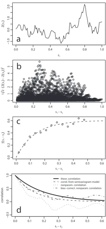
The customary procedure for estimating a semivariogram model is illustrated by means of synthetic data in Fig. 1a– c. Figure 1a shows a single realization of a one-dimensional Gaussian process with variance 1 and exponential correla-tion funccorrela-tion (the practical range equals 0.6 for this process). The sample semivariogram (or the so-called semivariogram cloud) is shown in Fig. 1b. It shows semivariogram ordi-nates for all pairs of observations. Since these values scatter substantially, the sample variogram is usually smoothed by calculating the estimate in Eq. (4) after pooling the semi-variogram ordinates into a number of lag-distance classes. This yields the so-called empirical semivariogram shown in Fig. 1c (open circles). Finally, a parametric model is fit to the empirical semivariogram. Here, a curve-fitting technique (n-weighted least squares, see Diggle and Ribeiro Jr, 2007, Sect. 5) has been used to estimate an exponential semivari-ogram model (dashed line in Fig. 1c). Equation (3) yields the parametric correlogram corresponding to the fitted semivari-ogram model (Fig. 1d, dashed line). The theoretical correla-tion funccorrela-tion is shown by the solid black line in Fig. 1d. The
0.0 0.2 0.4 0.6 0.8 1.0
−1.0
0.0
1.0
2.0
si
Z
(
si
)
0.0 0.2 0.4 0.6 0.8 1.0
012345
si−sj
1
2
(
Z
(
si
)
−
Z
(
sj
))
2
0.0 0.1 0.2 0.3 0.4 0.5 0.6
−0.5
0.0
0.5
1.0
si−sj
correlation
theor. correlation
correl. from semivariogram model nonparam. correlation
bias−correct. nonparam. correlation
a
b
c
d
0.0 0.1 0.2 0.3 0.4 0.5 0.6
0.0
0.2
0.4
0.6
si−sj
γ
^(
si
−
sj
)
Fig. 1. Semivariogram and correlogram estimation. (a)
One-dimensional synthetic data sample, (b) semivariogram cloud,
(c)empirical semivariogram and fitted parametric model,(d) the-oretical and estimated correlograms.
are chosen such that they fulfill the property of positive defi-niteness of the covariance matrix. Correlation functions with this property can be used in geostatistical prediction (Krig-ing; see relevant texts such as Schabenberger and Gotway, 2005, for details). Additionally, the parametrization further smoothes the empirical semivariogram and allows estimation of the correlation at unobserved lag distances.
2.2.2 Estimation of nonparametric correlograms
The nonparametric estimate of the correlation function is given by
ˆ
ρ(si−sj)= 1
N X N (si−sj)
Z(si)− ¯Z q
ˆ
C(0)
Z(sj)− ¯Z q
ˆ
C(0) where,
¯
Z= 1
N N X i=1
Z(si) and C(ˆ 0)= 1
N N X i=1
Z(si)− ¯Z2
(5) are the sample (also called plug-in) mean and variance, and Nis the number of observations (e.g., radar grid points). This estimator can be conveniently computed in terms of the dis-crete Fourier transform (DFT). In fact, the Wiener-Khinchin theorem affirms that the magnitude of the DFT of the stan-dardized observations is the spectral representation of the correlation estimate computed in Eq. (5). Thus, Eq. (5) can be obtained rather simply by computing the DFT, multiply-ing with the complex conjugate and computmultiply-ing the inverse DFT of the product. This has two main advantages. First, the fast Fourier transform (FFT) allows computing Eq. (5) much more rapidly than by means of explicit summation. There-fore, the complete radar grid can be taken into account. In contrast, the complete semivariogram estimator Eq. (4) can-not be conveniently computed for sizeable two-dimensional radar grids, and is practically obtained from “thinned-out” subsamples of the entire field (see Appendix A, Fig. A1, for an example). Second, the estimated correlation function has, by construction, a real and positive spectral density. Accord-ing to Bochner’s theorem, it is therefore a positive definite function (termed “licit” in Yao and Journel, 1998). No fur-ther fitting of a parametric covariance model or manipulation of the spectral density is necessary.
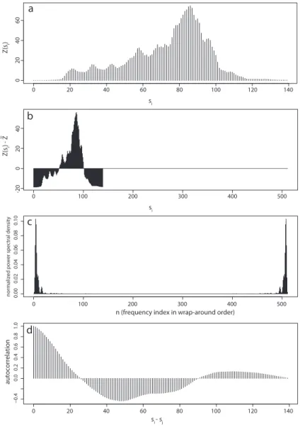
In practice, the mechanics of the FFT requires that the data be padded with zeros, and to switch to the so-called wrap-around order of spectral densities/lag distances and back. This is illustrated in Fig. 2 by means of a one-dimensional data sample; the details are explained in Press et al. (1992, Chapt. 13). The data sample of length N=140 is shown in (Fig. 2a). The mean is subtracted and zeros are padded such as to give a padded data vector (Fig. 2b) whose length is equal to the smallest power of 2 larger than or equal to 2N; here equal to 512. Application of the FFT, multiplica-tion with the complex conjugate, and normalizamultiplica-tion of the power spectral densities yields the result shown in Fig. 2c. The power spectral densities are obtained in the typical wrap-around order, i.e. the left part of the spectrum corresponds
to the zero frequency and positive frequencies, and the right part of the spectrum to negative frequencies (in reverse or-der). The spectrum is real, positive, and symmetric with re-spect to the zero frequency. Finally, the inverse FFT yields the estimate of the correlation function (Fig. 2d).
The nonparametric estimate Eq. (5) of the correlation function for the synthetic one-dimensional data sample of Fig. 1a is shown in Fig. 1d (dotted line).
2.2.3 Comparison of estimators and bias correction
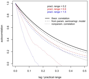
Both estimates of the correlogram function in Fig. 1d exhibit shorter ranges than the theoretical correlation. Of course, this could be completely due to sampling variability and we cannot conclude from the estimates for a single realization (Fig. 1a) on the behaviour of the estimators. Therefore, we extend the experiment as follows: for each of three Gaus-sian processes with unit variance and exponential correla-tion funccorrela-tion with practical ranges of 0.2, 0.6, and 1.5, we draw 100 realizations and estimate a parametric (exponen-tial) semivariogram model and the nonparametric correlation for each of the realizations. Each realization is sampled in the domain [0,1]. The median estimated parametric model for the process with practical range 0.2 is shown by the black dashed line in Fig. 3. This line is very close to the theoretical correlation (solid black line). As a matter of fact, the estima-tor Eq. (4) is known to be unbiased. For finite-size samples of correlated data, however, it is only approximately unbiased. In the present example, the positive autocorrelation causes the variance of the process (the semivariogram sill) to be un-derestimated. As a consequence, also the range of the semi-variograms is underestimated. This effect is the more pro-nounced the larger the practical range is compared to the do-main size, i.e. keeping the dodo-main size constant (here equal to 1), the bias will be larger for larger ranges (red and blue dashed lines in Fig. 3).
The dotted lines in Fig. 3 show the nonparametric corre-lation estimates from Eq. (5) based on the same 100 real-izations of the three Gaussian processes. For small lags and a practical range of 0.2, the estimate (black dotted line) is still fairly close to the theoretical correlation. If the practical range is on the order of the domain size, however, the non-parametric correlation is strongly biased towards too small values (red and blue dotted lines). The bias in the nonpara-metric correlogram estimate is much larger than in the corre-sponding parametric estimate. (Note: at least for small lags, the different normalizationsN (si−sj)vs.N in Eqs. (4) and (5) are only a minor contribution to the difference between both estimates.)
In order to understand this observation, we rewrite Eq. (5) as follows:
ˆ
ρ(si−sj)=1− 1− ˆρ(si−sj)
=1−
1− 1
NC(ˆ 0)
X
N (si−sj)
Z(si)− ¯Z
Z(sj)− ¯Z
si
Z(s
i
)
a
si b
−0.4
0.0
0.2
0.4
0.6
0.8
1.0
si - sj
autocorrelation
d
0 100 200 300 400 500
0.00
0.02
0.04
0.06
0.08
0.10
n (frequency index in wrap-around order) c
0
20
40
60
0 20 40 60 80 100 120 140
-20
0
20
40
0 100 200 300 400 500
0 20 40 60 80 100 120 140
Z(s
i
) - Z
normalized power spectral density
Fig. 2. Correlogram estimation using the fast Fourier transform.(a)One-dimensional section through the radar comopsite for test case 3 (6.33–8.13◦W at 46.39◦N; mm),(b)centered and zero-padded data,(c)normalized power spectral density in wrap-around order,(d) non-parametric estimate of the correlation function. Lags are in km.
=1−
ˆ
C(0)
2C(ˆ 0)+
ˆ
C(0)
2C(ˆ 0)−
1
NC(ˆ 0)
X
N (si−sj)
Z(si)− ¯Z Z(sj)− ¯Z
.
For lag distances that are much smaller than the domain di-mensions, we can approximate
ˆ
C(0)≈ 1
|N (si−sj)| X
N (si−sj)
Z(si)− ¯Z2 and
N≈ |N (si−sj)|.
Thus,
ˆ
ρ(si−sj)≈1− 1
2C(ˆ 0)|N (si−sj)|
X
N (si−sj)
Z(si)− ¯Z2
+
Z(sj)− ¯Z2
−2 Z(si)− ¯Z
Z(sj)− ¯Z ,
and finally
ˆ
ρ(si−sj)≈1−γ (ˆ si−sj)
ˆ
C(0) . (6)
Equation (6) shows that the calculation of a nonparametric correlogram is approximately equivalent to the estimation of a semivariogram, and the subsequent conversion of the semi-variogram to a correlogram using the simple plug-in estimate of the variance. If the interest is in estimating the correlation and variance of the process Z, the estimators Eq. (5) and
ˆ
0.0 0.1 0.2 0.3 0.4 0.5
0.0
0.2
0.4
0.6
0.8
1.0
lag / practical range
autocorrelation
pract. range = 0.2 pract. range = 0.6 pract. range = 1.5
theor. correlation
from param. semivariogr. model nonparam. correlation
Fig. 3. Behaviour of parametric and nonparametric correlogram es-timators for Gaussian spatial processes of different ranges. Dashed black line: Median fitted parametric model for a Gaussian process of practical range 0.2. Dotted black line: Median nonparametric correlogram estimate for a Gaussian process of practical range 0.2. Red and blue lines: the same for processes of larger practical ranges (0.6,1.5). All dashed and dotted lines show the median of estimates of 100 realizations of the Gaussian process. Solid line: theoreti-cal correlation (for all ranges; the abscissa is stheoreti-caled by the practitheoreti-cal range).
the extrapolation performed by fitting the parametric semi-variogram model. This explains the larger bias of the estima-tor in Eq. (5) compared to Eq. (4).
In the present context, the more important consequence of Eq. (6) is, however, that the nonparametric correlogram esti-mator Eq. (5) and the plug-in varianceC(ˆ 0)combine such as to yield an estimate of the semivariogramγ that is approx-imately unbiased for small lag distances. This is the justifi-cation for using these estimators for geostatistical prediction as done here as well as in earlier studies (notably Velasco-Forero et al., 2009). The semivariance provides a description of both the spatial dependence and the variance of the spatial field, and completely determines (jointly with the actual val-ues of the predictors) the solution of geostatistical prediction (Kriging).
Kriging will be the focus of the remainder of this paper. Before, we briefly digress and show how the bias of the esti-mator in Eq. (5) can be mitigated in situations where this is of interest. Given an alternative estimateσˆ2of the variance, assumed to be superior to the sample varianceC(ˆ 0), the cor-responding estimate of the correlation function is according to Eqs. (3) and (6):
ˆ
ρc(si−sj)=1−
ˆ γ (si−sj)
ˆ
σ2 ≈1−
ˆ C(0)
ˆ
σ2 1− ˆρ(si−sj)
. (7)
0.0 0.1 0.2 0.3 0.4 0.5
0.0
0.2
0.4
0.6
0.8
1.0
lag / practical range
autocorrelation
pract. range = 0.2 pract. range = 0.6 pract. range = 1.5
theor. correlation
from parametric semivariogram model bias−correct. nonparam. correlation
Fig. 4. As Fig. 3 but for bias-corrected nonparametric correlograms calculated according to Eq. (7).
For the synthetic data of our introductory example (Fig. 1a), we have used the sill of the parametric semivariogram (Fig. 1c) forσˆ2in Eq. (7) and the corrected correlation func-tion obtained in this way is the dash-dotted line in Fig. 1d. Repeating the experiment described at the beginning of this section with the bias-corrected estimator Eq. (7) yields the results shown in Fig. 4. Indeed, the correction works and the bias-corrected correlograms are very close to the paramet-ric correlograms for small lag distances. With increasing lag distance, the approximation the bias correction is based on deteriorates. This can be seen for the example with largest practical range (blue dotted line in Fig. 4). We have tested the calculation of bias-corrected correlograms not only for synthetic data but also for gridded radar precipitation fields. The test confirms that the bias correction works, i.e. that the bias-corrected nonparametric correlograms agree much bet-ter with the parametric correlograms than the uncorrected nonparametric correlograms (not shown).
2.3 Kriging formulations
In all Kriging applications, we are given k=1,...,K gauge measurementsZG(sk)andl=1,...,Lradar
measure-mentsZR(sl)at the grid points of the radar composite. We
associate all raingauges with the nearest radar pixel. The prediction locations coincide with the grid of the radar com-posite; for clearness we use superscripts whenever we refer to prediction locations, e.g.,sl. Throughout this study, we
work with a global Kriging neighbourhood and do not ap-ply any variable transformation to the predictors. Below we shortly describe how to calculate OK and KED predictions and variances; for more detailed descriptions of the methods the reader is referred to standard texts (e.g., Cressie, 1993; Wackernagel, 2003).
2.3.1 Ordinary Kriging
In all Kriging formulations, the process of the interpolated fieldZ(s)is modelled as the sum of a stochastic part, which
is a second-order stationary processY (s), and a deterministic
part. In OK, the deterministic part is assumed to be a constant mean fielda, i.e.
Z(s)=a+Y (s). (8)
The OK prediction is a weighted average of raingauge values ˆ
Z(sl)=
K
X
k=1
λlkZG(sk), (9)
and the optimal weightsλlkare the solution of the following systems of equations:
ˆ
C11 ··· ˆC1K 1
..
. . .. ... ... ˆ
CK1 ··· ˆCKK 1
1 ··· 1 0
=
λ11 ··· λL1 ..
. . .. ... λ1K ··· λLK µ1 ··· µL
ˆ
C11 ··· ˆC1L ..
. . .. ... ˆ
CK1 ··· ˆCKL 1 ··· 1
, (10)
where we have introduced the shorthand notation Cˆkk′=
ˆ
C(0)ρ(ˆ sk−sk′) for covariances between gauge locations,
ˆ
Ckl= ˆC(0)ρ(ˆ sk−sl)for covariances between gauge and
pre-diction locations, andµldenotes a Langrange multiplier that ensuresP
kλlk=1. The OK variance is given by
ˆ
σOK2 (sl)= ˆC(0)−µl−
K
X
k=1
λlkCˆkl. (11)
The covariances Cˆ in Eqs. (10) and (11) correspond to the stochastic model partY (s). In OK, it is natural to use
available measurements ofZfor the estimation of the spatial covariance structure ofY. Here, the covariances are esti-mated from the radar composites. We use a classical para-metric semivariogram fit with anisotropy (see Appendix A) as well as the nonparametric correlogram estimate (Eq. (5), Sect. 2.2.2). The corresponding OK versions are denoted by OKpand OKnp.
2.3.2 Kriging with external drift
In KED, the deterministic part of the model is supposed to be a linear function of an auxiliary field (here, the radar com-positeZR):
Z(s)=a+bZR(s)+Y (s). (12)
Just as in OK, the prediction is a weighted mean of raingauge values as in Eq. (9), but here the weights are the solution of the following systems of equations:
ˆ
C11 ··· ˆC1K 1R1
..
. . .. ... ... ...
ˆ
CK1 ··· ˆCKK 1RK
1 ··· 1 0 0 R1 ··· RK 0 0
=
λ11 ···λL1 .. . . .. ... λ1K ···λLK µ1
a ···µLa
µ1b ···µLb ˆ
C11 ··· ˆC1L .. . . .. ...
ˆ
CK1 ··· ˆCKL 1 ··· 1 R1 ···RL
, (13)
where we writeRk=ZR(sk)andRl=ZR(sl)for the radar values at the gauge and at the prediction locations. The addi-tional Lagrange multiplier ensures thatP
kλlkRk=Rl. The
KED variance is given by ˆ
σKED2 (sl)= ˆC(0)−µl
a−µlbRl−
K
X
k=1
λlkCˆkl. (14) A well known problematic issue in the application of KED is that there is no straightforward choice for which data to use to estimate the covariance structure of Y (s). The
es-timate would have to be based on residuals between an (a priori unknown) linear function of the radar field and an (a priori unknown) merged interpolated field. An elegant solu-tion to this problem is to fit the parameters of the stochastic and the deterministic part of the model jointly by means of maximum-likelihood methods (Diggle and Ribeiro Jr, 2007; Erdin, 2009); yet for sparse gauge networks and in situations with few wet radar-raingauge pairs, this estimation might not be very robust (In how far this is a problem for operational implementations is open. These methods are being tested in a separate activity within the CombiPrecip project.).
Here, we follow a different solution suggested by Velasco-Forero et al. (2009) that consists of the following steps:
1. A spatially complete rainfall field is estimated by OKnp using a sparse set ofradarvalues sampled at the gauge locations.
2. Use the residuals between the radar field and the predic-tion from step 1 to estimate the nonparametric correlo-gram and the variance ofY (s).
b
3ABO 0AIG 3ALT 0BAS 3BER 2BEZ 0BOU 0BUF 2BUS 1CDF 1CGI 1CHA 1CHU 5CHZ 0CIM 0COM 1COV 0DAV 1DIS 2DOL 6ENG 2EVO 0FAH 0FEY 3FRE 1GEN 6GLA 1GOE 3GRH 4GSB 3GUE 10GUT 1GVE 0HIR 0HOE 3INT 4KLO 1LEI 0LUG 10LUZ 0MAG 1MAH 3MLS 3MUB 0MVE 7NAP 2NEU 0OTL 0PAY 5PIL 0PIO 6PLF 2PSI 1PUY 4REH 0ROB 3ROE 0RUE 1SAE 0SAM 0SBE 0SBO 0SCU 5SHA 0SIO 16SMA 1STG 15TAE 1ULR 2VAD 1VIS 0WAE 0WFJ 2WYN 2ZER 0.5 2 4 6 8 10 12 14 16 20a
Test case 1: 2005-08-21 17:00-18:00 UTC
0ABO 0AIG 0ALT 0AND 1BAS 2BER 5BEZ 0BUF 0BUS 0CDF 0CGI 1CHA 0CHU 0CHZ 0CIM 0COM 0COV 0DAV 0DIS 0DOL 0ENG 0EVO 0FAH 0FRE 0GEN 0GLA 0GOE 0GRH 0GSB 0GUE 0GUT 0GVE 0HIR 6HOE 0INT 6KLO 0LEI 0LUG 0LUZ 0MAG 2MAH 0MLS 8MUB 0MVE 0NAP 1NEU 0OTL 2PAY 0PIL 0PIO 0PLF 0PSI 0PUY 0REH 0ROB 0ROE 0RUE 1SAE 0SAM 0SBE 0SBO 0SCU 0SHA 0SIO 0SMA 0STG 4TAE 0ULR 0VAD 0VIS 0WAE 0WFJ 0WYN 0ZER 0.5 2 4 6 8 10 12 16 20 24
c
d
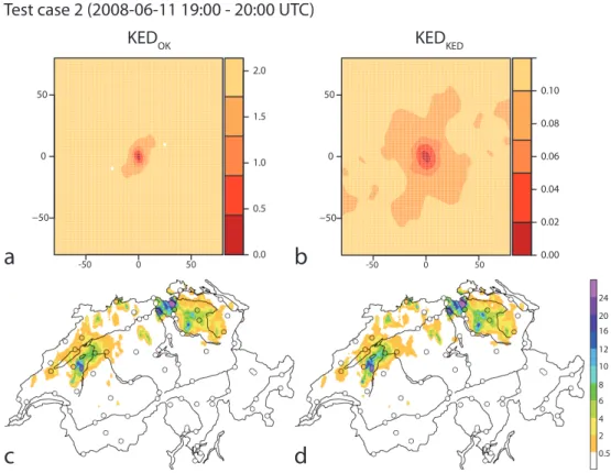
Test case 2: 2008-06-11 19:00-20:00 UTC
f
4ABO 4AIG 0ALT 0AND 0BAS 14BER 0BEZ 0BUF 1BUS 1CDF 0CGI 0CHA 0CHU 7CHZ 0CIM 0COM 0COV 0DAV 0DIS 0DOL 0ENG 0EVO 0FAH 0FRE 0GEN 0GLA 0GOE 1GRH 0GSB 0GUE 7GUT 0GVE 0HIR 3HOE 2INT 2KLO 1LEI 0LUG 1LUZ 0MAG 1MAH 1MLS 3MUB 0MVE 1NAP 0NEU 0OTL 1PAY 2PIL 0PIO 4PLF 0PSI 0PUY 8REH 0ROB 0ROE 1RUE 3SAE 0SAM 0SBE 0SBO 0SCU 2SHA 0SIO 10SMA 6STG 6TAE 0ULR 0VAD 0VIS 2WAE 0WFJ 1WYN 0ZER 0.5 4 8 12 16 20 24 28 32 36e
Test case 3: 2009-07-23 15:00-16:00 UTC
Fig. 5. Test cases considered in this study. (a, c, e)Hourly raingauge accumulations,(b, d, f)hourly radar accumulation; all in mm.
(a, b)August 2005 floods (test case 1),(c, d)EURO 2008 flooding (test case 2),(e, f)fast and heavy thunder cells with hail over the Swiss Plateau (test case 3).
1. Use KEDOKto obtain a preliminary prediction. 2. Use the residuals between the radar field and the
predic-tion from step 1 to estimate the nonparametric correlo-gram and the variance ofY (s).
3. Use the correlogram and variance obtained in step 2 for the KED prediction according to Eqs. (13) and (14). This is our second KED variant and we refer to it as KEDKED. The estimation of the covariance ofY (s)is still
pragmatic (we use the preliminary KEDOK prediction as a substitute of the interpolated target field and neglect the lin-ear function of the radar field), but we hypothesize that it yields a better description of the covariance ofY (s)than the OK residuals used in KEDOK.
2.4 Evaluation
2.4.1 Test cases
Examples of results from the Kriging variants will be shown for three test cases. Figure 5 shows raingauge (left) and radar (right) measurements for episodes of 1 h duration dur-ing these cases.
Test case 2 (Fig. 5c, d) is characterized by intense, short-lived, and localized precipitation cells in the northern part of Switzerland. One of these cells gained a certain fame be-cause of its interference with the football match Switzerland-Turkey at EURO 2008 in Basel. As far as the raingauge and radar accumulations for the corresponding hour are con-cerned, however, the effect of this cell is not very pro-nounced. The Basel gauge (at the northern border of Switzer-land, Fig. 5c) merely registered a value 1 mm for that hour. Much larger hourly accumulations can be seen in two sepa-rate regions in the northwest and the northeast of Switzer-land. Quite clearly, the gauge network is not sufficiently dense to capture the local precipitation maxima within these regions that are evident on the radar composite (Fig. 5d).
During the event of test case 3, heavy convective hail-storms moved over the Swiss Plateau at a speed of more than 60 kmh−1. The comparison of the daily radar and gauge data (not shown) shows that the spatial pattern is very similar be-tween both measurements, but the magnitude of the radar measurements is considerably higher than that of the gauges. This is a well-known phenomenon for radar measurements of hail (Doviak and Zrnc, 1993). Again, the gauges of the sparse real-time network do not capture the regions of strongest pre-cipitation for the selected hour (Fig. 5e, f). A closer inspec-tion of the radar composite shows an artificially rugged struc-ture due to the fact that precipitation cells displace substan-tially between consecutive full scan periods of the radar (see also Fabry et al., 1994).
2.4.2 Cross validation
We use cross validation for the quantitative evaluation of the different merging techniques. One gauge is removed from the data in turn, and the prediction of the method under con-sideration is then compared to the value measured by the re-moved gauge. Since correlograms or semivariograms are es-timated from the radar field for all methods considered here, the correlograms and semivariograms are the same in cross validation as for the complete set of gauges. In the KEDOK and KEDKEDmethods that involve auxiliary initial steps for the construction of a residual field used to estimate nonpara-metric correlograms, the cross-validated gauge is only re-moved in the final Kriging step.
This kind of leave-one-out cross validation with compari-son to gauges is probably the most popular procedure in the evaluation of combination techniques for raingauge and radar data. Among the numerous studies that have applied cross validation are Seo (1998), Haberlandt (2007), and DeGae-tano and Wilks (2009). Nevertheless, some critical issues should be born in mind in this analysis:
– Gauge values are assumed to be true values at their spe-cific locations, but include measurement errors for sev-eral reason (Sevruk, 1985). These errors are assumed to be small compared to the prediction errors in the precip-itation fields at short time scales. For particular cases
(snowfall, strong wind), however, these errors can be substantial and should be considered in principle (Al-though a quantitative correction is hardly possible.).
– A representative spatial distribution of gauges is neces-sary to assess the average performance of a method in the study area. As far as the distribution over differ-ent parts of the country is concerned, the MeteoSwiss raingauge network reasonably meets this requirement. Remote and high-altitude locations, however, are some-what underrepresented.
– The spatial and temporal support of radar and rain-gauges is different. Spatially, rainrain-gauges can be approx-imated as point measurements, whereas the radar values correspond to averages over the volume of a grid cell. This yields to a smoothing of radar values compared to gauges (Zawadzki, 1975). Thus, differences between raingauge and radar measurements are not solely due to radar errors, but also due to differences in representa-tiveness.
– Additional uncertainty is introduced by associating the location of a raingauge with the centre of the nearest radar grid cell (nearest-neighbour approximation). These issues illustrate that care should be excercised when interpreting radar-raingauge differences. Nevertheless, under the assumption that these effects lead primarily to a random component in the radar-raingauge differences, comparisons over a large sample of raingauges still provide useful guid-ance on the relative performguid-ance of different merging tech-niques.
2.4.3 Quality measures
Skill statistics are calculated from gauge observation/cross-validation prediction pairs{Zi,Zˆi}, wherei,...,Ienumerates
all such pairs either for a single test case or for an extended validation period. We use the following skill measures:
1. The BIAS assesses overall systematic errors of a method. We express it in terms of a logarithmic scale, as customary in radar meteorology,
BIAS=10 log10
P
iZˆi
P
iZi
. (15)
2. The root-mean-square error (RMSE) is a widely-used skill measure to assess the overall quality of a method. We use it on a square-root scale,
RMSE=
v u u t
1 I
X
i
q
ˆ Zi−
p
Zi
2
Table 1. 2×2 contigency table for the calculation of HK from observation-prediction pairs{Zi,Zˆi}.
Zwet Zdry Sum
ˆ
Zwet a b a+b
ˆ
Zdry c d c+d
Sum a+c b+d I
3. The median absolute deviation (MAD) is a robust mea-sure of dispersion, i.e. it is less influenced by outliers than the RMSE:
MAD=median
i
|
q
ˆ Zi−
p
Zi|
. (17)
4. SCAT (Germann et al., 2006) evaluates the performance of a method to quantify precipitation for locations where rain is actually predicted and observed. SCAT is based on the cumulative error distribution function (CEDF), defined as the contribution to total precipitation as a function of the logarithmic prediction-observation ratio (in dB) at locations where both, observation and pre-diction are wet (≥0.5 mm). SCAT is defined as half the distance between the 16 % and 84 % quantiles of the CEDF, which makes it robust to outliers with large over-or underestimation. The observed CEDF points are in-terpolated linearly to determine the required quantiles;
SCAT=1
2(CEDF84−CEDF16) . (18)
5. The Hansen-Kuipers Discriminant (HK) is a skill score to assess dichotomous predictions. In our context, it can be used to measure the ability of a method to distinguish between dry and wet areas. We define a dry observation to correspond to<0.5mm and a wet observation to≥ 0.5mm. Observation-prediction pairs{Zi,Zˆi}can then
be used to construct a 2×2 contigency table (Table 1) and HK is calculated as
HK= ad−bc
(a+c)(b+d) . (19)
This is equal to the Probability of Detection (POD) minus the Probability of False Detection (POFD), and −1≤HK≤1. HK=0 means that the forecast is as skillful as a random forecast, HK=1 is a perfect fore-cast, and a negative HK implies a forecast worse than random.
We compute all of the above skill measures for the three test cases, and throughout an extended evaluation period. All hourly intervals in 2008 with at least one wet gauge (≥0.5mm) and without missing values in the radar com-posite are included into the extended evaluation. We find
that the first four scores, especially MAD, are hard to in-terpret if many observation-prediction pairs with very small values are included into the evaluation. Therefore, we only include pairs with gauge observationZ≥0.5mm in the cal-culation of the scores 1–3. For these three scores, this leaves 52/13/30 pairs of values for test cases 1/2/3. The calculation of HK is based on all observation-prediction pairs (75 for the test cases). As far as the results for the extended evalu-ation period are concerned, the scores are calculated from a large number of pairs (37 416 for BIAS, RMSE, MAD, and SCAT; and 222 013 for HK). The constraint of allow-ing radar fields without any missallow-ing radar pixel only reduces the evaluation period to 10 months (there are missing values in April and May 2008). Nonetheless, the results from the extended evaluation are highly significant and approximately represent averages across all seasons.
2.4.4 Evaluation of Kriging uncertainty
A potential advantage of geostatistical merging techniques is that they are based on a stochastic concept. They not only yield an interpolated field, but also an estimate of the uncertainty in this interpolation at each grid point. In par-ticular, following the cross-validation approach described in Sect. 2.4.2, a measure of uncertainty – the cross-validation Kriging variance – can be calculated at the location of the removed gauge. This can be used to assess how useful the uncertainty estimate provided by the different methods is. More specifically, we test if the Kriging variance along with a Gaussian assumption on the distribution of errors can be used to construct an accurate confidence interval at a point. To this end, we calculate for each gauge and throughout the extended evaluation period a z-scoreZˆi−Zi
/σˆi, where
ˆ
Zi andσˆi2are the cross-validation prediction and variance,
andZi is the value measured by the removed gauge. Then,
the frequency of threshold exceedances ofzcan be compared with the frequency that is expected under the assumption of a standard Gaussian distribution ofz.
3 Results
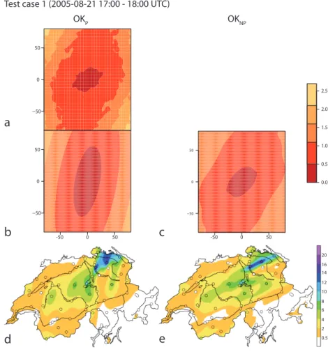
3.1 Test case 1
Test case 1 (2005-08-21 17:00 - 18:00 UTC)
OKP OKNP
20 16 14 12 10 8 6 4 2 0.5 0.0 0.5 1.0 1.5 2.0 2.5
−50 0 50
−50 0 50
-50 0 50
−50 0 50
-50 0 50
a
b
c
d
e
Fig. 6. Ordinary Kriging for test case 1 with a parametric semivariogram (OKp) and a nonparametric correlogram (OKnp). (a)Empirical semivariogram from subsampled radar field (mm2),(b)exponential anisotropic semivariogram fit (mm2),(c)nonparametric correlogram from complete radar field (expressed as a semivariance, mm2),(d)OKpprediction,(e)OKnpprediction (mm).
accomodate different directions of anistropy. Instead, the fit-ted semivariogram model is a compromise between different directions (expressed by means of a single anisotropy angle) and strengths (expressed by means of a single anisotropy ra-tio). In this particular example, the fit result appears to be in-fluenced more by the larger lag distances than by the values of the empirical semivariogram near the origin. In Ordinary Kriging from a sparse network, the semivariogram model has a very strong influence on the Kriging prediction, and indeed we can clearly see its imprint in Fig. 6d. The comparison to the radar field for this case (Fig. 5b) suggests that the OKp prediction does not represent the spatial characteristics for this rainfall field very well. The dominant rainfall patterns and their orientation, in particular the narrow band of in-tense precipitation in the northeast of Switzerland, are not captured.
The result of the nonparametric correlogram fit – con-verted into a semivariogram using the plug-in estimate of the variance of the radar field – is shown in Fig. 6c. The non-parametric semivariogram naturally represents the change of
the anisotropy angle with lag distance and no decisions about which lags to give preference have to be made, since the non-parametric semivariogram is used directly in Kriging. Even though radar information is only incorporated via the semi-variogram, the OKnpprediction (Fig. 6e) is able to reproduce the narrow precipitation band and compares much better to the original radar field. The cross-validation results corrobo-rate what the visual inspection of the results suggests for this example: all skill measures yield a better score for OKnpthan for OKp(Table 2).
d
20 16 14 12 10 8 6 4 2 0.5
a
c
-50 0 50 −50
0 50
0.0 0.1 0.2 0.3 0.4
-50 0 50 −50
0 50
0.0 0.5 1.0 1.5
b
Test case 1 (2005-08-21 17:00 - 18:00 UTC)
KEDOK KEDKED
Fig. 7. Kriging with external drift for test case 1 (left: KEDOK, right: KEDKED).(a)Nonparametric correlogram for KEDOKexpressend as a semivariogram (mm2),(b) nonparametric correlogram for KEDKED expressed as a semivariogram (mm2), (c)KEDOK prediction,
(d)KEDKEDprediction (mm).
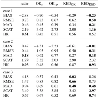
Table 2. Cross-validation skill measures for the original radar field and different merging techniques for the three test cases.
radar OKp OKnp KEDOK KEDKED
case 1
BIAS −2.88 −0.90 −0.54 −0.29 −0.23
RMSE 0.73 0.83 0.67 0.62 0.50
MAD 0.46 0.45 0.39 0.34 0.21
SCAT 2.19 3.62 2.73 2.00 1.16
HK 0.61 0.45 0.51 0.56 0.52
case 2
BIAS 0.47 −4.51 −3.23 −0.61 −0.01
RMSE 0.44 1.03 0.95 0.50 0.31
MAD 0.18 0.62 0.77 0.27 0.18
SCAT 1.79 3.52 3.03 2.90 2.32 HK 0.93 0.48 0.56 0.87 0.93
case 3
BIAS 4.18 −0.57 −0.43 −0.02 0.26
RMSE 1.47 0.83 0.82 0.66 0.73 MAD 0.94 0.69 0.61 0.48 0.48
SCAT 3.49 3.38 3.85 3.42 2.97
HK 0.67 0.67 0.52 0.69 0.74
d
24
20
16
12
10
8
6
4
2
0.5
a
b
c
e
−500 50
0 1 2 3 4 5
−50 0 50
-50 0 50 -50 0 50
−50 0 50
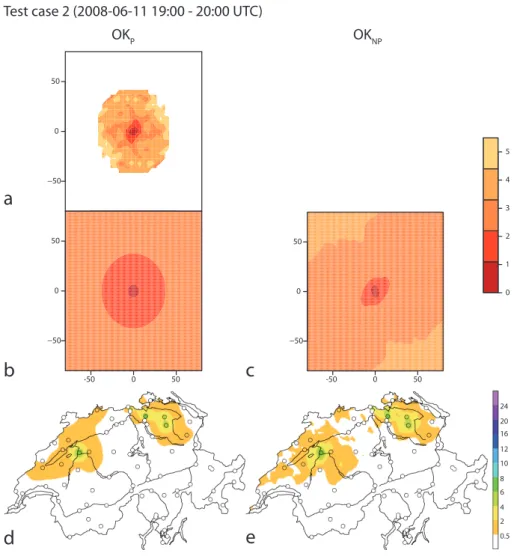
Test case 2 (2008-06-11 19:00 - 20:00 UTC)
OKP OKNP
Fig. 8. As Fig. 6 but for test case 2.
improved estimates in many respects; but that the distinction of wet and dry areas is best in the pure radar measurements.
3.2 Test case 2
The isolated patches of high precipitation in the radar com-posite for test case 2 (Fig. 5d) suggest that the spatial depen-dence is of short range. This is well captured by the paramet-ric semivariogram fit (Fig. 8b) and also by the semivariogram based on the nonparametric correlogram estimate (Fig. 8c). While the parametric semivariogram is completely isotropic, the nonparametric semivariogram exhibits some short-range anisotropy the orientation of which again changes with lag distance. The dominant anisotropy of this semivariogram at short lags appears to reproduce that of three adjacent patches of high precipitation at the northern border of Switzerland. All in all, however, anisotropy is not as important here as in the other two test cases as evident in the OK predictions (Fig. 8d, e). The fit of a simple monotonously decaying function (here exponential) for the parametric semivariogram
yields a smoother prediction by OKp than by OKnp. The more irregular character of the OKnpprediction better agrees with the original radar composite, even though, of course, the precise location and shape of precipitating areas is not cap-tured well since the radar is not a proper predictor variable in the OK methods. The skill measures for OKpand OKnp do not differ greatly for this test case. Compared to other methods/test cases, both OK methods exhibit a large nega-tive bias, arguably due to the fact that areas of high precipi-tation are simply “overlooked” in interpolation from a sparse gauge network and for a case with small-scale precipitation patterns.
d
24
20
16
12
10
8
6
4
2
0.5
a
c
b
-50 0 50
0.0 0.5 1.0 1.5 2.0
−50 0 50
0.00 0.02 0.04 0.06 0.08 0.10
−50 0 50
-50 0 50
Test case 2 (2008-06-11 19:00 - 20:00 UTC)
KED
OK
KED
KEDFig. 9. As Fig. 7 but for test case 2.
case, and also quite similar to one another. Consequently, the evaluation results are also quite similar for these three fields.
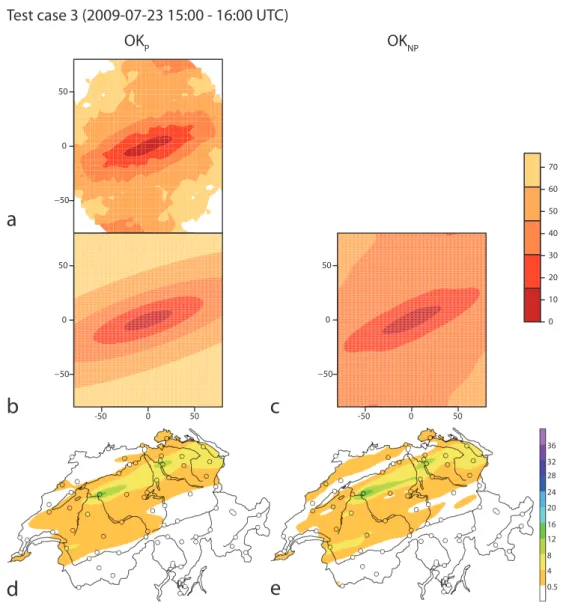
3.3 Test case 3
The spatial dependence structure for this test case is largely determined by three bands of intense precipitation that are aligned fairly similarly in a southwest-northeasterly direction (Fig. 5f). Here, the assumption of a domain-wide spatial de-pendence model and the description of anisotropy in terms of a single anisotropy ratio and angle, appears to be much better suited than for the test cases discussed above. Indeed, the parametric semivariogram model agrees quite well with the semivariogram based on the nonparametric correlogram estimate for small lag distances (Fig. 10b, c), even though the range is larger for the latter. Consequently, also the OK pre-dictions are all in all rather similar (Fig. 10d, e), yet for OKnp the impact of individual raingauge values on the interpolated field can be discerned at larger lag distances. This can be seen clearly for the station Bern (“BER”) in the centre/west of Switzerland that registered an accumulation of 14 mm of rain during the hour of this test case (Fig. 5e) and the band of high precipitation to its west in the OK predictions (Fig. 10d, e). This band is more pronounced for the OKnp prediction than for OKp and remarkably similar in shape to the cor-responding band actually observed in the radar composite (Fig. 5f). The cross-validation results for the two OK
predic-tions (Table 2) are in line with the apparent similarity of the two fields: while some of the skill measures yield favourable results for OKnp (BIAS, MAD), others give preference to OKp(SCAT, HK).
As in the previous test cases, the KED combination meth-ods succeed to incorporate the fine-scale spatial detail of the radar and at the same time correct for the substantial bias (here positive) of the radar with respect to the gauges. This is evident from the inspection of the predicted fields (Fig. 11c, d) and also from the quantitative evaluation (Table 2). In cross-validation, the KED methods score better than the OK predictions and also than the original radar field, even in terms of the distinction of dry and wet locations measured by HK. While for the previous test cases the KEDKED pre-dictions receive higher scores than KEDOKpredictions, there is no clear picture for this test case. The semivariograms for KEDOKand KEDKED (Fig. 11a, b), determined from differ-ent residual fields, have an anisotropy similar to the semivar-iograms for OKpand OKnp(Fig. 10b, c), but quite naturally, the semivariogram sills and ranges are smaller than for the OK semivariograms, which are based on the original radar field. This observation holds also for the other two test cases.
3.4 Systematic evaluation
d
36
32
28
24
20
16
12
8
4
0.5
a
b
c
e
-50 0 50 -50 0 50
−50 0 50
0 10 20 30 40 50 60 70
−50 0 50
−50 0 50
Test case 3 (2009-07-23 15:00 - 16:00 UTC)
OK
P
OK
NPFig. 10. As Fig. 6 but for test case 3.
performance of a merging technique from the consideration of one or a few examples. Therefore, we have also conducted the evaluation through an extended period of time both for the Kriging prediction (best estimate) and the Kriging vari-ance as described in Sects. 2.4.2–2.4.4. Due to the compara-tively slow estimation of the empirical semivariogram in the OKpmethod, this method is not included into the extended evaluation.
3.4.1 Kriging best estimate
The evaluation results for the original radar field and the three merging techniques are summarized in Table 3. The skill measures in this table assess the performance of the tech-niques in average terms across a large number of cases as well as across different regions of Switzerland. The evalua-tion results are unequivocal. The average performance of the
d
36
32
28
24
20
16
12
8
4
0.5
a
c
b
-50 0 50
0 5 10 15
−50 0 50
0 5 10 15 20 25
−50 0 50
-50 0 50
Test case 3 (2009-07-23 15:00 - 16:00 UTC)
KED
OK
KED
KEDFig. 11. As Fig. 7 but for test case 3.
Table 3. Cross-validation skill measures for the original radar field and different merging techniques for the extended evaluation in 2008.
radar OKnp KEDOK KEDKED
BIAS −1.16 −1.29 −0.92 −0.60
RMSE 0.61 0.51 0.47 0.39
MAD 0.38 0.27 0.26 0.20
SCAT 2.86 2.61 2.35 1.91
HK 0.59 0.64 0.68 0.73
many precipitation occurrences in these regions, which ap-pears to be the reason for the rather low HK score. (In fact, the spatially varying radar skill also partly explains the dif-ferences between the radar skill for the different test cases. The radar skill is much higher for test case 2 than for the other two cases, arguably because in this case it did not rain in regions where the radar skill is typically rather low.).
Figure 12 shows the results of the extended evaluation for the RMSE on a station by station basis. In accord with the above discussion, the radar skill is comparatively low in re-mote regions of complex topography (Fig. 12a). The OKnp method (Fig. 12b) introduces an improvement in the skill that is fairly homogeneous throughout the country. It is
interest-ing to compare the two KED methods the RMSE of which is shown in Fig. 12c, d. Both methods have markedly bet-ter skill (lower RMSE) than OKnpin regions where the radar performs well, in the Swiss middleland in the centre/north of the country. For KEDKED however, RMSE is also sub-stantially reduced in the mountainous regions in the south of Switzerland, much more so than for KEDOK. This observa-tion appears to justify the hypothesis we made when intro-ducing the KEDKEDmethod in Sect. 2.3.2. In regions where the radar is a powerful predictor variable, the stochastic part of the geostatistical model is less decisive for the prediction skill and, accordingly, the KEDOK and KEDKED methods perform similarly. In regions where the quality of the radar is lower, the quality of the prediction will depend more on the specification of the stochastic part of the model. This is consistent with the clearly superior performance of KEDKED in these regions.
3.4.2 Kriging uncertainty
Radar OK C
KED
OK KEDKED
0.3 0.38 0.46 0.54
a
b
c
d
Fig. 12. RMSE (mm0.5) for extended evaluation in 2008 by gauge station.
the gauge locations due to the fact that no nugget effect is taken into account by the correlograms used herein.
The results of evaluating the Kriging variance for the OKnp method are shown in Fig. 14. In the cross-validation analy-sis, we have computed a series ofz-scores for each gauge as explained in Sect. 2.4.4. Figure 14a shows for each gauge, how often thez-score is found to be smaller than the 5 %-quantile of the standard Gaussian distribution, which is ap-proximately equal to−1.64. This corresponds to situations where the value predicted by OKnp substantially underesti-mates the actually observed value (by more than 1.64 times the Kriging standard deviation). Under the assumptions of a well estimated Kriging variance and a Gaussian distribu-tion of errors, this is expected to occur in 5 % of the cases. But in fact the probability of underestimating is drastically larger than expected under these assumptions (Fig. 14a). In other words, if a confidence interval was constructed from the Kriging variance and under the assumption of Gaussian error distribution, the upper end of this confidence interval would be too small. The OKnpmethod misses the peaks of the gridded field more often than suggested by the geosta-tistical model. As far as overestimations are concerned, the observed occurrence frequencies differ substantially from the expected value at a few gauges, yet this effect is less severe than for the underestimations (Fig. 14b).
We have also assessed the uncertainty estimates provided by the KEDOK and KEDKED methods. The results (not shown) are very similar to those shown for OKnpin Fig. 14, but the overestimation occurrence frequencies are somewhat ‘worse’ (higher) than the corresponding frequencies shown in Fig. 14a for OKnp. Several reasons must be expected to contribute to the poor quality of the uncertainty estimate of
the methods tested here. In all methods, we have used the radar and raingauge dataas is, i.e. we have made no effort to apply a variable transformation (e.g., the Box-Cox trans-formation) such as to make the residuals of the geostatistical models follow a Gaussian distribution. In fact, given the high skewness of hourly precipitation data it would be quite sur-prising to find that the residuals of the untransformed data are Gaussian. It is our current working hypothesis, that the missing data transformation is a major reason for the poor uncertainty estimate. Accordingly, the choice of an appro-priate transformation family and the estimation of the trans-formation from the data on a case-by-case basis constitute a separate effort within the CombiPrecip project running in parallel to this study. Further issues that may contribute to the deterioration of the uncertainty estimate are the quality of the approximation in Eq. (6) and, for the KED methods, the pragmatic choice of residual fields used to estimate the nonparametric correlogram. The fact that the assessment of the Kriging uncertainties yields rather similar results for the OKnp, KEDOK, and KEDKEDmethods, indicates that the ef-fect of the last issue is comparatively small.
4 Findings summary and discussion
In this study, we have tested using nonparametric correlo-grams for the construction of hourly gridded precipitation fields obtained from the geostatistical combination of rain-gauge and radar data in Switzerland.
1 0.8 0.6 0.4 0.2
c
d
Test case 1 (2005-08-21 17:00 - 18:00 UTC)
KED
OK KEDKED
a
b
OK
P OKNP
Fig. 13. Square root of the Kriging variance for the test case 1 and OK and KED method variants (mm).
0.01 0.1 0.2 0.5
P(z < -1.64)
P(z > 1.64)
a
b
OK
NP 31 24 19 21 16 26 25 26 23 30 13 35 24 19 28 26 29 24 18 54 29 22 28 36 38 28 16 49 59 37 19 28 34 30 24 12 27 29 25 30 19 22 19 34 31 26 48 16 53 22 28 34 35 15 44 67 16 62 27 42 47 26 23 1825 26 29
29 14 22 26 39 20 22 22 3 3 10 2 1 16 2 3 4 3 25 6 4 12 36 14 17 14 10 3 8 7 3 4 16 7 8 6 0 8 7 3 13 4 6 9 6 19 19 14 13 7 2 1 4 5 13 5 6 17 3 10 2 10 1 1 10 6 5 8 11 2 5 7
5 5 11
13 17 8 3 6 5 5 9
Fig. 14. Assessment of the Kriging variance for the OKnp method. At each gauge location the color and numbers (%) show(a)the relative frequency of underestimating the precipitation by 1.64 standard deviations or more,(b)the relative frequency of overestimating the precipitation by 1.64 standard deviations or more. The analysis includes all gauge observations≥0.5 mm.
known correlation structure has shown that the nonparamet-ric correlograms may severly underestimate the decorrelation length (the range of the correlogram). This estimation bias is greater, the smaller the dimensions of the data sample are in relation to the actual range of the spatial dependence. The bias in the correlogram is mostly due to the fact that the cor-relogram estimate is based on the sample (“plug-in”) vari-ance as an estimate of the varivari-ance of the spatial field. For positively correlated data, the sample variance may substan-tially underestimate the process variance, much more so than the semivariogram sill traditionally used in geostatistical ap-plications.
We have also compared the nonparametric correlogram estimation with the traditional semivariogram estimation by using them in Ordinary Kriging of gauges for three Com-biPrecip test cases. The estimation of nonparametric cor-relograms (more precisely, of semivariograms based on the nonparametric correlograms) is very attractive from an oper-ational point of view since (i) the entire spatially complete radar field can be taken into account, (ii) no parametric semi-variogram model has to be fitted, and (iii) the estimation of the nonparametric correlogram is fast and robust. For the three test cases considered here, OK in terms of the nonpara-metric correlogram (method OKnp) successfully captures the spatial dependence structure of the radar field. A quantitative comparison of the OKnpmethod with OK in terms of the tra-ditional parametric semivariogram (method OKp) has shown that OKnp performs similarly to or better than OKpfor the three test cases.
Furthermore, two variants of Kriging with external drift have been tested in this study. The first variant is the method suggested by Velasco-Forero et al. (2009), termed here KEDOK. The second variant builds on the KEDOK method and constructs a more realistic residual field used to estimate the nonparametric correlogram of the stochastic part of the KED model. Both variants have been assessed by means of cross-validation and a range of skill measures through an extended evaluation period of one year. The re-sults clearly show that KEDKED yields better merged pre-cipitation fields than KEDOK on average. Additionally, the extended evaluation shows that both KED methods perform better than the original radar composite or the gauge interpo-lation OKnp.
We have also assessed the uncertainty estimate provided by the OKnp, KEDOK, and KEDKED methods. All three methods underestimate the precipitation amount more often than expected from the Kriging variances and the assump-tion of a Gaussian error distribuassump-tion. Consequently, uncer-tainty estimates for the methods presented here should be based on the empirical error distribution rather than on the Kriging variances.
A number of issues have not been addressed in this study and remain for current and future work. It is conceivable that the failure of the uncertainty estimate of the present imple-mentations is largely due to the fact that no variable transfor-mation is applied to the precipitation data. Finding a suitable transformation on a case-by-case basis constitutes a part of the CombiPrecip project in its own right. Given the practi-cal advantages of the nonparametric correlogram estimation, it appears promising to test if a data transformation can be incorporated into the methods presented here (in particular KEDKED).
As explained in Sect. 2.4.2, the cross-validated gauge is only removed in the final Kriging step in cross validation of the KEDOKand KEDKEDmethods. We do not expect this to have a substantial influence on the evaluation results. Even though somewhat involved, the whole purpose of steps 1 and
2 of the KEDOK and KEDKED methods is to yield residual fields from which the nonparametric correlograms forY(s) (Eqs. 8 and 12) can be estimated. The presence or absence of a single gauge should only have a minor influence on the general character of these correlograms. On a similar note, Erdin (2009) found for the combination of daily Swiss radar and raingauge data, that re-estimating a parametric semivari-ogram for each gauge removed in leave-one-out cross valida-tion differs negligibly from the result obtained using the full set of raingauges. Nonetheless, the sparser gauge network used herein, the characteristics of the spatial distribution of hourly precipitation, and the ability of nonparametric correl-ograms to capture much of the actual spatial structure, might have some impact on how a single gauge can influence the estimated correlogram. We plan to quantify this in future im-plementations.
A potential disadvantage of nonparametric correlograms is that they can only be used when a complete spatial field is available for estimating the spatial dependence structure of the stochastic part of the geostatistical model under consider-ation. While this is straightforward for Ordinary Kriging, we have shown that in other Kriging formulations the choice of an appropriate field is much less clear. Moreover, the meth-ods tested in this study assume that the estimation of the spa-tial dependence structure and the parameters of the determin-istic part of the geostatdetermin-istical model can be carried out in two consecutive independent steps. This appears to be at odds with modern geostatistical estimation techniques (maximum-likelihood or reduced maximum (maximum-likelihood), where both the parameters of the deterministic part of the model and of the spatial covariance structure are estimated jointly. An itera-tive approach such as the KEDKED method suggested here may be a first step towards methods that self-consistently es-timate both the deterministic part of the geostatistical model and the spatial covariance of the stochastic part, but still take advantage of the computational convenience offered by the nonparametric estimation of correlograms.
Appendix A
Estimation of parametric semivariograms with anisotropy
The procedure used for the estimation of parametric semivar-iograms with anisotropy consists of five steps. It is illustrated in Fig. A1 for test case 3.
0 50 100
01
02
03
04
05
0
u
γ
σ2=54.6 mm2
φ =26.3 km
u
v
−50 0 50
−50 0 50
0 10 20 30 40 50 60 70 80 90
u
v
−50 0 50
−50 0 50
0 10 20 30 40 50 60 70 80 90
u
v
−50 0 50
−50 0 50
0 10 20 30 40 50 60 70 80 90
b
c
d
e
0.5 4 8 12 16 20 24 28 32 36
a
Test case 3 (2009-07-23 15:00 - 16:00 UTC)
Fig. A1. Estimation of a two-dimensional parametric semivariogram. (a)Subsample of 3370 random radar pixels from the full composite of CombiPrecip test case 8 (Fig. 5f; mm).(b)First-guess one-dimensional semivariogram from the subsample,(c)two-dimensional sample variogram,(d)two-dimensional variogram restricted to small lags,(e)exponential anisotropic variogram model fitted to the central part of the sample variogram.
2. As described in Sect. 2.2.1, a one-dimensional omnidi-rectional semivariogram is fit to the sample variogram obtained from the radar subsample drawn in step 1 (Fig. A1b). We choose an exponential model
ˆ
γ (u)= ˆσfg2 1−exp u ˆ φfg
!!
, (A1)
whereu= |si−sj| is the lag distance; and thus
ob-tain first-guess estimates of the varianceσˆfg2 and of the range parameterφˆfg. The one-dimensional sample
var-iogram is calculated from data pairs of a maximum lag distanceumax=150km, and the exponential model is fit to the sample variogram by means of ann-weighted least-squares method (Diggle and Ribeiro Jr, 2007, sec-tion 5.3.1). The practical range isuˆ⋆fg.
3. A two-dimensional sample semivariogram is calculated from the radar subsample according to Eq. (4), here un-derstood as a function of a two-dimensional lag vec-tor u=(u,v). The sample variogram is computed