SCALABLE AND PRECISE RANGE ANALYSIS
RAPHAEL ERNANI RODRIGUES
SCALABLE AND PRECISE RANGE ANALYSIS
ON THE INTERVAL LATTICE
Dissertação apresentada ao Programa de Pós-Graduação em Ciência da Computação do Instituto de Ciências Exatas da Univer-sidade Federal de Minas Gerais como req-uisito parcial para a obtenção do grau de Mestre em Ciência da Computação.
Orientador: Fernando Magno Quintão Pereira
Belo Horizonte
RAPHAEL ERNANI RODRIGUES
SCALABLE AND PRECISE RANGE ANALYSIS
ON THE INTERVAL LATTICE
Dissertation presented to the Graduate Program in Computer Science of the Fed-eral University of Minas Gerais in partial fulfillment of the requirements for the de-gree of Master in Computer Science.
Advisor: Fernando Magno Quintão Pereira
Belo Horizonte
© 2014, Raphael Ernani Rodrigues. Todos os direitos reservados.
Rodrigues, Raphael Ernani
R696s Scalable and Precise Range Analysis on the Interval Lattice / Raphael Ernani Rodrigues. — Belo Horizonte, 2014
xxviii, 79 f. : il. ; 29cm
Dissertação (mestrado) — Universidade Federal de Minas Gerais
Orientador: Fernando Magno Quintão Pereira
1. Computação — Teses. 2. Compiladores — Teses. I. Orientador. II. Título.
This work is dedicated to my parents, friends, professors and fellows, who have supported me throughout this journey. They have provided me with the vital conditions to accomplish this mission.
Acknowledgments
I’m grateful to my family, my friends, my professors, and my fellows at the university. My family, specially my parents Gleyce and David, have provided the conditions for me to continue studying. They gave me a suitable environment, and allowed me to abstract from the bureaucracy of life in order to focus on my M.Sc. I am unconditionally grateful for all they have done for me since I was born.
My friends gave me pretty happy days. That was surely important for me to finish this program. Without their companionship, my days would be lonely, sad and dark, and I would not have psychological stability to finish this work.
My professors have guided me through this journey, pointing the dead ends and the promising opportunities. I’m very thankful for all their help, specially for the wise words and patience of Fernando, my adviser. His words have encouraged me to continue advancing, even during the hardest days and most difficult challenges of this long path. Laure Gonnord, from École Normale Supérieure de Lyon, also deserves special recognition for having nearly adopted me in my academic internship in Lyon.
I’m also thankful for the company of my fellows in the university. Igor Rafael deserves special thanks for giving me valuable tips about the life as a graduate student. In addition, also the loyal boys who inhabit the lab at room 3054 deserve special thanks, because they made not only my days better, but the M.Sc. as a whole a pleasant experience.
Finally, I must recognize the importance of CAPES and PPGCC to my formation. CAPES have provided the financial aid that allowed me to exclusively dedicate my time to the master’s program. PPGCC have provided the formal conditions in the academic system. The good job done by PPGCC members have made my life easier as a student and let me keep focus on the really important things.
“To become an expert, you have to master the fundamentals”
(Stephen Gilbert & Bill McCarthy)
Resumo
Uma análise de largura de variáveis é um algoritmo que estima o menor e o maior valor que cada variável em um programa de computador pode assumir durante a execução deste programa. Este tipo de análise provê informação que permite ao compilador entender melhor os programas e realizar uma série de otimizações.
Muito trabalho já foi realizado no projeto e implementação de análises de largura de variáveis. Entretanto, soluções anteriores existentes na literatura têm sua aplicação prática bastante restrita, porque se baseiam em abordagens que são muito caras ou muito imprecisas.
Neste trabalho é apresentada uma implementação de análise de largura de var-iáveis que é atualmente o estado-da-arte neste campo de pesquisa, oferecendo o melhor balanço entre velocidade de análise e precisão de resultados.
Este trabalho também apresenta exemplos onde o uso da análise de largura de variáveis contribui para segurança computacional, projeto de hardware e otimização de programas.
Acreditamos que esta obra descreve a exploração mais completa dos benefícios da análise de largura de variáveis em programas grandes, presentes no mundo real.
Palavras-chave: Compiladores, Análise de Largura de Variáveis, Análise estática, Otimização.
Abstract
A Range analysis is a technique that estimates the lowest and highest values that each variable in a computer program may assume during an execution of the program. This kind of analysis provides information that helps the compiler to better understand and optimize programs.
There has been much work in the design and implementation of range analyses. However, previous works have found limited practical application, because they rely on approaches that are either expensive or imprecise.
In this work we present an implementation of range analysis that is currently the state-of-art in this field of research, and provides the best balance between speed and precision.
We also present examples where the use of our range analysis contributes to software security, hardware design and program optimizations.
We believe that this work describes the most extensive exploration of the benefits of range analysis in large, real-world, programs.
Palavras-chave: Compilers, Range Analysis, Static Analysis, Optimization.
Extended Abstract
A Range Analysis (RA) is an algorithm that estimates the lowest and highest values that each integer variable in a computer program may assume during an execution of the program. This kind of analysis provides information that helps the compiler to better understand and optimize programs.
However, previous works rely on approaches that are either expensive or impre-cise, limiting their practical application. In this work we present an implementation of a new range analysis that is currently among the best tools of its kind publicly available. Our implementation provides the best balance between speed and precision. By relying on an idea that we deem future values - a key insight of our algorithm - we produce fast results that are comparable to the precision of more expensive solutions. We also present the advantages of the application of our range analysis in different scenarios:
1. In computing security, to provide efficient protection against undefined be-haviour caused, for instance, by integer overflows or access beyond the bounds of an array. Integer overflow occurs when a variable assumes a value that does not fit in the precision of the data type used for the variable while array-bound errors occur when accesses to an array continue beyond the end of the array. Our RA was applied successfully to remove unnecessary safety verifications in programs, enhancing the performance of safe programs.
2. In hardware design, to reduce the storage space and the wiring necessary to store a variable. RA can be used to prove that a given variable will not use the en-tire width of the data type assigned to it in the program. Therefore that variable can be stored into smaller registers and can use fewer lines to be transmitted be-tween different areas of the processing element. The bitwidth reduction enabled by the RA produces faster programs that make a better use of the hardware and save energy.
3. In static program analysis, to expand the scope and improve the precision of static analysis routinely applied to code by optimizing compilers. A more precise RA can be used to infer the outcome of conditional tests in a program. For instance, with proven range bounds for the value of variables, a dead-code elimination may be able to prove more code to be dead, a constant-propagation may be able to propagate constants further, and an alias analysis may be able to reduce the size of alias sets. More precise alias sets may enable further data restructuring and automatic parallelization transformations that make better use of the memory hierarchy and of multi-core processor architectures.
In this work we present many contributions related to our range analysis. First, we present a new range analysis algorithm that relies on future values – the key insight of our algorithm – to gain precision without resorting to expensive techniques. Second, we present a technique to secure programs against integer overflows and show how we can use the RA to avoid inserting unnecessary checks. Third, we present u-SSA, a new program representation that is based on overflow-free programs and increases the precision of the RA. Finally, we present an heuristic to estimate the number of iterations of loops, based on patterns of variable updates.
This work summarizes a two years long effort that pushes the state of the art of the range analyses into a new level and demonstrates that it can be successfully used by program optimizations to produce smaller and faster machine code.
List of Figures
2.1 Example program. . . 11
3.1 (a) Example program. (b) SSA form [Cytron et al. [1991]]. (c) e-SSA form [Bodik et al. [2000]]. (d) u-SSA form. . . 19 3.2 Growth on the number of instructions in comparison with SSA representation. 21
4.1 A suite of constraints that produce an instance of the range analysis problem. 24 4.2 (a) Example program. (b) Control Flow Graph in SSA form. (c) Constraints
that we extract from the program. (d) Possible solution to the range analysis problem. . . 25
4.3 Our implementation of range analysis. Rounded boxes are optional steps. . 26 4.4 (a) The control flow graph from Figure 4.2(b) converted to standard e-SSA
form. (b) A solution to the range analysis problem . . . 27
4.5 The dependence graph that we build to the program in Figure 4.4. . . 28 4.6 (Left) The lattice of the growth analysis. (Right) Cousot and Cousot’s
widening operator. We evaluate the rules from left-to-right, top-to-bottom, and stop upon finding a pattern matching. Again: given an interval ι = [l, u], we let ι↓ =l, andι↑ =u . . . 30
4.7 Rules to replace futures by actual bounds. . . 30 4.8 Cousot and Cousot’s narrowing operator. . . 30
4.9 Four snapshots of the last SCC of Figure 4.4. (a) After removing control dependence edges. (b) After running the growth analysis. (c) After fixing the intersections bound to futures. (d) After running the narrowing analysis. 31
4.10 Correlation between program size (number of var nodes in constraint graphs after inlining) and analysis runtime (ms). Coefficient of determination = 0.967. . . 33
4.11 Comparison between program size (number of var nodes in constraint graphs) and memory consumption (KB). Coefficient of determination = 0.9947. . . 33 4.12 (Upper) Comparison between static range analysis and dynamic profiler
for upper bounds. (Lower) Comparison between static range analysis and dynamic profiler for lower bounds. The numbers above the benchmark names give the number of variables in each program. . . 34 4.13 Design space exploration: precision (percentage of bitwidth reduction)
ver-sus speed (secs) for different configurations of our algorithm analyzing the SPEC CPU 2006 integer benchmarks. . . 36 4.14 Strongly Connected Components extracted from our example program. . . 36 4.15 (Left) Time to run our analysis without building strong components divided
by time to run the analysis on strongly connected components. (Right) Precision, in bitwidth reduction, that we obtain with strong components, divided by the precision that we obtain without them. . . 37 4.16 (Left) Bars give the time to run analysis on e-SSA form programs divided
by the time to run analysis on SSA form programs. (Right) Bars give the size of the e-SSA form program, in number of assembly instructions, divided by the size of the SSA form program. . . 38 4.17 The impact of the e-SSA transformation on precision for three different
benchmark suites. Bars give the ratio of precision (in bitwidth reduction), obtained with e-SSA form conversion divided by precision without e-SSA form conversion. . . 39 4.18 Example where an intra-procedural implementation would lead to imprecise
results. . . 40 4.19 Example where a context-sensitive implementation improves the results of
range analysis. . . 41 4.20 The impact of inter-procedural analysis on precision. Each bar shows
pre-cision in %bitwidth reduction. . . 41 4.21 (Left) Runtime comparison between intra, inter and inter+inline versions
of our algorithm. (Right) Runtime comparison between different widening operators. The bars are normalized to the time to run the intra-procedural analysis. . . 42 4.22 An example where jump-set widening is more precise. . . 43
5.1 An example of an exploitable integer overflow vulnerability. . . 46
5.2 Overflow checks. We use ↓n for the operation that truncates to n bits. The subscript s indicates a signed instruction; the subscript u indicate an unsigned operation. . . 47 5.3 Number of instructions used in each check. . . 48 5.4 (a) A simple C function. (b) The same function converted to the LLVM
intermediate representation. (c) The instrumented code. The boldface lines were part of the original program. . . 49 5.5 Percentage of overflow checks that our range analysis removes. Each bar is
a benchmark in the LLVM test suite. Benchmarks have been ordered by the effectiveness of the range analysis. On average, we have eliminated 24.93% of the checks (geomean). . . 52 5.6 Comparison between execution times with and without pruning, normalized
by the original program’s execution time. . . 54
6.1 (a)Example program. (b) CFG of the program, after conversion to SSA form. (c)Dependence graph highlighting nodes that do not affect the loop predicate, after converting the original program into . . . 56 6.2 (a)Dependence graph. (b)Multi-node SCC of the variable i1. (c)Sequence
of redefinitions of the variablei1. (d)Effect of one iteration on the variable i1 59 6.3 Lattice of SR classifications. . . 60
List of Tables
3.1 Impact of the transformation to e-SSA and u-SSA in terms of program size. # SSA: number of instructions in the SSA form program. # e-SSA: number of instructions in the e-SSA form program. # u-SSA: number of instructions in the u-SSA form program. . . 20
4.1 Variation in the precision of our analysis given the widening strategy. The size of each benchmark is given in number of variable nodes in the constraint graph. Precision is given in percentage of bitwidth reduction. Numbers in parenthesis are percentage of gain over 0 + Simple. . . 43
5.1 Instrumentation without support of range analysis. #I: number of LLVM bitcode instructions in the original program. #II: number of instructions that have been instrumented. #O: number of instructions that actually overflowed in the dynamic tests. . . 51 5.2 Instrumentation library with support of static range analysis. #II:
num-ber of instructions that have been instrumented without range analysis. #E: number of instructions instrumented in the e-SSA form program. #U: number of instructions instrumented in the u-SSA form program. . . 52 5.3 How the range analysis classified arithmetic instructions in the u-SSA form
programs. #Sf: safe. #S: suspicious. #U: uncertain. #SO: number of suspicious instructions that overflowed. #UO: number of uncertain instruc-tions that overflowed. . . 53
6.1 Natural Loops in the Control Flow Graph. L: number of natural loops. NL: number of nested loops. SEL: number of loops that have a single exit point. 65 6.2 Classification of Natural Loops according to their stop conditions. L:
num-ber of natural loops. IL: numnum-ber of Interval Loops. EL: number of Equality Loops. OL: number of Other Loops. . . 65
6.3 Classification of Strongly Connected Components in the Dependence Graph. SN: number of Single-Node SCCs. MN: number of Multi-Node SCCs. SP: number ofSingle-PathSCCs. MP: number ofMulti-PathSCCs. SL: number of Single-Loop SCCs. NL: number ofNested-Loop SCCs. . . 66 6.4 Trip Count Instrumentation. IL: interval loops. IIL: instrumented interval
loops. EL: equality loops. IEL: instrumented equality loops. . . 67 6.5 Trip Count Profiler - Trip count estimated using vectors. . . 69 6.6 Trip Count Profiler - Trip count estimated using simplified heuristic. . . . 69
Contents
Acknowledgments xi
Resumo xv
Abstract xvii
Extended Abstract xix
List of Figures xxi
List of Tables xxv
1 Introduction 1
1.1 Range Analysis . . . 1 1.2 Integer Overflows . . . 2 1.3 Trip Count Prediction . . . 3 1.4 Contributions . . . 3 1.5 Experimental results . . . 5 1.6 Publications and Software . . . 6
2 Literature review 9
2.1 Range Analysis . . . 9 2.2 Live Range Splitting . . . 11 2.3 Integer Overflows . . . 12 2.4 Trip Count Analysis . . . 14
3 Live Range Splitting 17
3.1 Live Splitting Alternatives . . . 17 3.2 Experiments . . . 20 3.3 Conclusion . . . 21
4 Range Analysis 23
4.1 Background . . . 23 4.3 Our Design of a Range Analysis Algorithm . . . 25 4.3.1 Finding Ranges in Strongly Connected Components . . . 29 4.3.2 Experiments . . . 32 4.4 Design Space . . . 35 4.4.1 Strongly Connected Components . . . 35 4.4.2 The Choice of a Program Representation . . . 37 4.4.3 Intra versus Inter-procedural Analysis . . . 39 4.4.4 Achieving Partial Context-Sensitiveness via Function Inlining . . 40 4.4.5 Choosing a Widening Strategy . . . 42 4.5 Conclusion . . . 44
5 Integer Overflows 45
5.1 The Dynamic Instrumentation Library . . . 46 5.2 Experimental Results . . . 50 5.3 Conclusion . . . 53
6 Trip count prediction 55
6.1 Background . . . 55 6.1.1 Natural Loops . . . 56 6.1.2 Strongly Connected Components . . . 57 6.1.3 Sequences of Redefinitions of Variables . . . 58 6.1.4 Vectors . . . 60 6.1.5 Patterns of movement . . . 60 6.2 A Trip Count Algorithm Based on Vectors . . . 61 6.3 A Simplified Trip Count Algorithm Based on Vectors for JIT compilers 63 6.4 Experimental Results . . . 64 6.5 Conclusion . . . 69
7 Final considerations 71
7.1 Future Works . . . 71 7.2 Conclusions . . . 72
Bibliography 73
Chapter 1
Introduction
Range analysis is a compiler technique whose objective is to determine, statically, for each program variable, limits for the minimum and maximum values that this variable might assume during the program execution. In this work we propose a new range analysis algorithm that has linear space and time complexity and has a precision that is comparable to that of more expensive analyses. We also present a technique to secure programs against integer overflows. Furthermore, we show how we use our range analysis to eliminate unnecessary integer overflow checks. Finally, we present an algorithm to estimate the trip count of loops – the number of iterations that the loops of a program execute. We use parts of our range analysis to be more accurate in our estimates.
1.1
Range Analysis
The analysis of integer variables on the interval lattice has been the canonical exam-ple of abstract interpretation since its introduction in the seminal paper of Cousot and Cousot [1977]. Optimizing compilers use range analysis to infer the possible values that discrete variables may assume during program execution. This analysis has many uses. For instance, it allows the optimizing compiler to remove from the program text redun-dant overflow tests and unnecessary array bound checks(Bodik et al. [2000]; Gampe et al. [2011]). Furthermore, range analysis is essential to bitwidth aware register allo-cators (Barik et al. [2006]; Tallam and Gupta [2003]), register alloallo-cators that handle registers of different sizes (Kong and Wilken [1998]; Pereira and Palsberg [2008]; Scholz and Eckstein [2002]), and scratchpad cache allocators (Yang et al. [2011]). Addition-ally, range analysis has also been used to statically predict the outcome of branches (Patterson [1995]), to detect buffer overflow vulnerabilities (Simon [2008]; Wagner et al.
2 Chapter 1. Introduction
[2000]), to find the trip count of loops (Lokuciejewski et al. [2009]) and even to syn-thesize hardware (Cong et al. [2005]; Lhairech-Lebreton et al. [2010]; Mahlke et al. [2001]).
Given this great importance, it comes as no surprise that the compiler literature is rich in works describing in details algorithmic variations of range analyses (Mahlke et al. [2001]; Gawlitza et al. [2009]; Stephenson et al. [2000]; Su and Wagner [2005]). On the other hand, none of these authors provide experimental evidence that their approaches are able to deal with very large programs. There are researchers who have implemented range analyses that scale up to large programs (Patterson [1995]; Blanchet et al. [2003]; Venet and Brat [2004]); nevertheless, because the algorithm itself is not the main focus of their works, they neither give details about their design choices nor provide experimental data about it. This scenario was recently changed by Oh et al. [2012], who introduced an abstract interpretation framework which processes programs with hundreds of thousands of lines of code. Nevertheless, Oh et al. have designed a simple range analysis, which does not handle comparisons between variables, for instance. They do not discuss the precision of their implementation, but only its runtime and memory consumption. In this work we claim to push this discussion considerably further.
1.2
Integer Overflows
The most popular programming languages, including C, C++ and Java, limit the size of primitive numeric types. For instance, the int type, in C++, ranges from −231
to
231
−1. Consequently, there exists numbers that cannot be represented by these types. In general, these programming languages resort to a wrapping-arithmetics semantics (Warren [2002]) to perform integer operations. If a number n is too large to fit into a primitive data typeT, then n’s value wraps around, and we obtain n modulo Tmax. There are situations in which this semantics is acceptable, like Dietz et al. [2012] has shown. For instance, programmers might rely on this behavior to implement hash func-tions and random number generators. On the other hand, there exists also situafunc-tions in which this behavior might lead a program to produce unexpected results. As an example, in 1996, the Ariane 5 rocket was lost due to an arithmetic overflow – a bug that resulted in a loss of more than US$370 million (Dowson [1997]).
bina-1.3. Trip Count Prediction 3
ries derived from C, C++ and Java programs to detect the occurrence of overflows dynamically. Thus, the instrumented program can take some action when an overflow happens, such as to log the event, or to terminate the program. However, this safety has a price: arithmetic operations need to be surveilled, and the runtime checks cost time. Zhang et al. [2010] have eliminated some of this overhead via a tainted flow analysis. We have a similar goal, yet, our approach is substantially different.
1.3
Trip Count Prediction
Loops represent most of the execution time of a program. For that reason, there is a well-known aphorism that says that "all the gold lays in the loops", because compiler optimizations made inside loops have their benefits multiplied by the number of iterations actually executed. As a consequence of that fact, there is a vast number of works in the literature that are specialized in loop optimizations, like the ones described by Kennedy and Allen [2001] and Wolfe et al. [1995].
Some optimizations, however, are highly sensitive to the number of iterations of a given loop. For instance, if a given loop iterate a few times in an interpreter, an aggressive optimization made by a Just-In-Time (JIT) compiler may not even pay for the compilation overhead. On other hand, if the same loop iterates thousands of times, the JIT compilation might use more expensive techniques and still have a better end-to-end performance. The number of iterations a loop actually executes is called
Trip Count. Here we use the same concept of trip count as described by [Wolfe et al., 1995, pp.200]. This number is only known at runtime, as it depends on the state of the variables of the program immediately before the loop starts.
Rice [1953] has demonstrated that predicting this information is an undecidable problem. Therefore, we can develop either a conservative solution or an heuristic to solve this problem. In this work, we present a heuristic that extracts patterns of the updates of variables’ values and estimates the trip count of loops with symbolic expressions. Those expressions might, then, be evaluated at runtime and allow the compiler to decide dynamically what code to execute depending on the actual expected number of iterations.
1.4
Contributions
4 Chapter 1. Introduction
engineering choices. Our range analysis relies on a three-phase algorithm that results in good precision without resorting to expensive methods. Second, we present a tech-nique to detect integer overflows and protect programs against them. We have used our range analysis to prove that some instructions will never cause integer overflows. Then, we can avoid inserting unnecessary checks in those instructions. Third, we present u-SSA, a new program representation that provides more information about the variables of overflow-free programs than previous representations. Finally, we bring a new algorithm to estimate the trip count of loops. Our trip count predictor uses the range analysis during the process of extracting symbolic expressions from the loops, representing its estimated trip counts.
Range Analysis: Our first algorithmic contribution on top of previous works is a three-phase approach to handle comparisons between variables without resorting to any exponential time technique. The few publicly available implementations of range analyses that we are aware of, such as those in FLEX 1
, gcc 2
or Mozilla’s IonMonkey 3
only deal with comparisons between variables and constants. Even theoretical works, such as Su and Wagner [2005] or Gawlitza et al. [2009] suffer from this limitation. This deficiency is one of the reasons explaining why none of these works has made their way into industrial-strength compilers. Two other insights allow our implementation to scale up to very large programs. We use Bodik’s Extended Static Single Assignment (e-SSA) form (Bodik et al. [2000]) to perform path-sensitive range analysis sparsely. This program representation ensures that the interval associated with a variable is constant along its entire live range. Finally, we process the strongly connected components that underline our constraint system in topological order. It is well-known that this technique is essential to speedup constraint solving algorithms ([Nielson et al., 1999, Sec 6.3]); however, due to our three-phase approach, a careful propagation of information along strong components not only gives us speed, but also improves the precision of our results.
Integer Overflow Checks: Our second algorithmic contribution is a tech-nique to identify integer overflows in programs. Like Dietz et al. [2012] and Brumley et al. [2007], we insert dynamic checks inside the code of the target programs. Our dynamic checks use the resulting value of the integer instructions and their operands to
1
The MIT’s FLEX/Harpoon compiler provides an implementation of Stephenson’s algorithm (Stephenson et al. [2000]), and is available athttp://flex.cscott.net/Harpoon/.
2
Gcc’s VRP pass (athttp://gcc.gnu.org/svn/gcc/trunk/gcc/tree-vrp.c) implements a vari-ant of Patterson’s algorithm (Patterson [1995]).
3
1.5. Experimental results 5
decide whether an overflow has occurred or not. This, of course, creates an undesired overhead during the runtime. However, we have noticed that a large number of checked instructions never actually overflow. We, then, use our range analysis to identify those instructions that are guaranteed to never overflow and avoid inserting overflow checks in them. By pruning the unnecessary checks, we were able to eliminate part of the overhead, which means that we have increased the efficiency of the safe programs. Our experiments show that the overhead that our remaining overflow checks cause is negligible.
u-SSA - A new program representation: Our third contribution is a pro-gram representation that extends Bodik’s e-SSA and provides additional information about variables of programs that are safe against integer overflows. We have observed that some properties hold when we ensure that the program terminates in face of integer overflows. Thus, we have extended e-SSA and included more divisions in the live range of variables that allow us to increase the precision of our range analysis.
Trip count prediction: Our fourth algorithmic contribution is an heuristic to compute the symbolic trip count of loops. This information is important to estimate the complexity of the program and to let the compiler to generate different code for loops that will iterate small or large numbers of times. As the exact static computation of the trip count of loops is impossible, there is no optimal algorithm to solve this problem. Therefore, in this work we propose a new heuristic to estimate such number of iterations. Our algorithm identifies patterns under which the variables are updated between two iterations and derives vectors that represent how the variable move over the real line. When we know how the variables move, we can estimate the number of iterations needed for them to reach a termination state.
1.5
Experimental results
We have implemented our algorithms in the LLVM compiler (Lattner and Adve [2004]), and have used it to process a set of benchmarks with 2.72 million lines of C code.
6 Chapter 1. Introduction
obtained via a dynamic profiler, which we have also implemented. As we show in Section 4.3.2, when analyzing well-known numeric benchmarks we are able to estimate tight ranges for almost half of all the integer variables present in these programs. Our results are similar to Stephenson et al. [2000], even though our analysis does not require a backward propagation phase. Furthermore, we have been able to find tight bounds to the majority of the examples used by Costan et al. [2005] and Lakhdar-Chaouch et al. [2011], who rely on more costly methods.
Integer Overflow Checks: We use our range analysis to reduce the runtime overhead imposed by a dynamic instrumentation library. This instrumentation framework, which we describe in Section 5.1, has been implemented in the LLVM compiler. We have logged overflows in a vast number of programs, with special focus on SPEC CPU 2006 benchmarks. We have re-discovered the integer overflows recently observed by Dietz et al. [2012]. The performance of our instrumentation library, even without the support of range analysis, is within the 5% runtime overhead of Brumley et al. [2007]’s state-of-the-art algorithm. The range analysis halves down this overhead. Our static analysis algorithm avoids 24.93% of the overflow checks created by the dynamic instrumentation framework. With this support, the instrumented SPEC programs are only 1.73% slower. Therefore, we show in this paper that securing programs against integer overflows is very cheap.
Trip count prediction: As we show in Section 6.4, our trip count heuristics present a good balance between speed and precision. The simpler analysis, that aims JIT compilers, has been shown to offer a good precision, even without the use of our Range Analysis. It was able to infer bounds for 75% of the loops of our benchmarks, of which 66% was shown to be precise by our profiler. Our second analysis, that is more elaborated and aims regular compilers, has been shown to be even more precise. We have been able to provide bounds to 75% of the loops, of which 75% was shown to be precise. Similar works, such as Gulwani et al. [2009a]’s are able to provide symbolic bounds to 90% of the loops, but rely on a much more expensive technique, that limits their application to smaller programs.
1.6
Publications and Software
1.6. Publications and Software 7
range analysis algorithm and presents the engineering choices we have made. It also brings the experimental results of our implementation. In chapter 4 we provide more details about the algorithm and its experimental results. The second one, "A fast and low-overhead technique to secure programs against integer overflows" (Rodrigues et al. [2013]), presents our technique to identify integer overflows and to secure programs against them. The third one, "Prevenção de Ataques de Não-Terminação baseados em Estouros de Precisão" (Rodrigues and Pereira [2013]) shows how our technique to secure programs against integer overflows can be used to avoid non-termination in programs. Chapter 5 extends the discussion presented in the papers about integer overflow handling.
Two other papers containing our trip count algorithm are currently under de-velopment. The first one describes in details our algorithm, engineering choices and results. The second one, "Selective Page Migration in ccNUMA Systems", is the result of a joint effort with researchers from UNICAMP and ETH Zurich. It shows how our trip count prediction can be used to make a more efficient use of the memory hierar-chy. Both papers are being prepared to be submitted to international conferences in February 2014.
Software: All the software produced during the research of this work is pub-licly available at http://code.google.com/p/range-analysis. In our website we
Chapter 2
Literature review
In this chapter we discuss a list of works that are strongly related to our studies. Our goal here is to evaluate the previous results available in the literature and show where we have made advances. Thus, in section 2.1 we discuss briefly how our Range Analysis algorithm overcome previous approaches and what are its limitations. We also evaluate the evolution of the program representations, that have created suitable conditions to develop our algorithm. Section 2.3 shows the works with goals that are similar to our integer overflow protection. Finally, section 2.4 discusses the papers in the literature that are related to our trip count heuristics.
2.1
Range Analysis
In this section we make the literature review of works related to our Range Analysis. We discuss how our Range Analysis is compared with previous analyses available in the literature. In addition, we show how the area has evolved along the decades and how we place our contribution in this evolution. Furthermore, we compare our approach with existing alternatives, both in terms of scalability and precision.
Range analysis is an old ally of compiler writers. The notions of widening and narrowing were introduced by Cousot and Cousot [1977] in one of the most cited papers in computer science. Different algorithms for range analysis have been later proposed by Patterson [1995], Stephenson et al. [2000], Mahlke et al. [2001] and many other researchers. Recently there have been many independent efforts to find exact, polynomial time algorithms to solve constraints on the interval lattice, as we can see in Gawlitza et al. [2009], Su and Wagner [2005], Costan et al. [2005], Lakhdar-Chaouch et al. [2011], and Su and Wagner [2004]. However, these works are still very theoretical, and have not yet been used to analyze large programs. Contrary to them, our approach
10 Chapter 2. Literature review
has a strong practical engineering bias and is shown to be able to analyze programs with millions of assembly instructions in less than 15 seconds.
The abstract interpretation framework introduced by Cousot and Cousot [1977] does not apply only to range analysis. It was initially designed for safety proofs, because of its capability of extracting properties of variables, functions or even entire programs without executing the source code. Those properties could, then, be used to find errors at compile time, as we can see in the works of Clarke et al. [1994] and Flanagan et al. [2002]. Furthermore, abstract interpretation is used in many data flow analyses, such as Liveness Analysis, Available Expressions, Reaching Definitions and Constant Propagation [Schwartzbach, 2008, pp.17].
There have been many practical approaches to abstract interpretation, with special emphasis on range analysis, such as Gampe et al. [2011] , Blanchet et al. [2003], Bertrane et al. [2010], Cousot et al. [2009] and Jung et al. [2005]. Cousot’s group,for instance, has been able to globally analyze programs with thousands of lines of code, albeit using domain specific tools. The tool Astrée, for example, only analyzes programs that do not contain recursive calls. The work that is the closest to ours is the recent abstract interpretation framework of Oh et al. [2012]. Oh et al. discuss an implementation of range analysis on the interval lattice that scales up to a program with1,363KLoC (ghostscript-9.00). Because their focus is speed, they do not provide results about precision. We could not find the benchmarks used in those experiments for a direct comparison – the distribution of ghostscript-9.00 available in the LLVM test suite has 27KLoC. On the other hand, we globally analyzed our largest benchmark, SPEC CPU 2006’s 403.gcc, enabling function inlining, in less than 15 seconds. 403.gcc has 521KLoC and, during our analysis, 1,419K LLVM IR instructions. Oh et al.’s implementation took orders of magnitude more time to go over programs of similar size. However, whereas they provide a framework to develop general sparse analyses, we only solve range analysis on the interval lattice.
There are in the literature works that are more powerful than ours. Figure 2.1 shows an example that illustrates one limitation of our approach. In this example, variablesi and sare initialized with the same value and are always updated together.
However, becausei ands does not have any syntactic dependence, our range analysis
gives the range[0,10]for variableiand[0,+∞]for variables. Nevertheless, relational
2.2. Live Range Splitting 11
Figure 2.1. Example program.
2.2
Live Range Splitting
In this work we present a sparse implementation of range analysis. Sparsity, in our context, means that we associate points in the lattice of interest – intervals in our case – directly to variables. Dense analyses map such information to pairs formed by variables and program points. The compiler related literature contains many descriptions of sparse data-flow analyses. Some among these analyses obtain sparsity by using specific program representations, like we did. Others rely on structures. In terms of data-structures, the first, and best known method proposed to support sparse data-flow analyses is the Sparse Evaluation Graph (SEG) of Choi et al. [1991]. The nodes of this graph represent program regions where information produced by the data-flow analysis might change. Choi et al.’s ideas have been further expanded, for example, by the Quick Propagation Graphs of Johnson and Pingali [1993], or the Compact Evaluation Graphs of Ramalingam [2002]. Building upon Choi’s pioneering work, researchers have developed many efficient ways to build such graphs. Examples of that can be found in Pingali and Bilardi [1995], Pingali and Bilardi [1997], and Johnson et al. [1994]. These data-structures have been shown to improve many data-flow analyses in terms of runtime and memory consumption. Nevertheless, the elegance of SEGs and its successors have not, so far, been enough to attract the attention of mainstream compiler writers. Compilers such as gcc, LLVM or Java Hotspot rely, instead, on several types of program representations to provide support to sparse data-flow analyses.
Most eminent among these representations is the Static Single Assignment form presented by Cytron et al. [1991], which suits well forward flow analyses, such as
12 Chapter 2. Literature review
Information (SSI) form, a program representation that supports both forward and backward analyses. This representation was later revisited by Singer [2006] and, a few years later, by Boissinot et al. [2009]. Singer provided new algorithms plus examples of applications that benefit from the SSI form, and Boissinot et al., in an effort to clarify some misconceptions about this program representation, introduced the notions of weak and strong SSI form. Another important representation, which supports data-flow analyses that acquire information from uses, is the Static Single Use form (SSU). There exists many variants of SSU, as shown in the works of Plevyak [1996], George and Matthias [2003], and Lo et al. [1998]. For instance, the “strict” SSU form enforces that each definition reaches a single use, whereas SSI and other variations of SSU allow two consecutive uses of a variable on the same path. The program representation that we have used in this work – the Extended Static Single Assignment (e-SSA) form – was introduced by Bodik et al. [2000]. The program representation
There are so many different program representations because they fit specific data-flow problems. Each representation, given a domain of application, provides the following property: the information associated with the live range of a variable is invariant along every program point where this variable is alive. There are two key as-pects that distinguish one representation from the others: firstly, where the information about a variable is acquired, and secondly, how this information is propagated. The e-SSA form, for instance, supports flow analyses that obtain information both from variable definitions and conditional tests and propagate this information forwardly. Such analyses are also supported by the SSI form; hence, we could have used this other representation too. However, Tavares et al. [201X] have shown in previous work that the e-SSA form is considerably more economical.
2.3
Integer Overflows
In this work we use the Range Analysis to eliminate unnecessary integer overflow checks. By doing this, we are entering in a completely different field of research. Thus, in this section we show what other researchers have already presented in this area. We compare our solution with the previously existing ones.
2.3. Integer Overflows 13
integer overflows. The author’s approach consists in instrumenting every integer operation that might cause an overflow, underflow, or data loss. The main result of Brumley et al. is the verification that guarding programs against integer overflows does not compromise their performance significantly: the average slowdown across four large applications is 5%. RICH uses specific features of the x86 architecture to reduce the instrumentation overhead. Chinchani et al. [2004] follow a similar approach, describing each arithmetic operation formally, and then using characteristics of the computer architecture to detect overflows at runtime. Differently from these previous works, we instrument programs at LLVM’s intermediate representation level, which is machine independent. Nevertheless, the performance of the programs that we instrument is on par with Brumley’s, even without the support of the static range analysis to eliminate unnecessary checks. Furthermore, our range analysis could eliminate approximately 45% of the runtime overhead that the tests that a naive implementation of Brumley’s technique would insert.
Dietz et al. [2012] have implemented a tool, IOC, that instruments the source code of C/C++ programs to detect integer overflows. They approach the problem of detecting integer overflows from a software engineering point-of-view; hence, perfor-mance is not a concern. The authors have used IOC to carry out a study about the occurrences of overflows in real-world programs, and have found that these events are very common. It is also possible to implement a dynamic analysis without instrument-ing the target program. In this case, developers must use some form of code emulation. Chen et al. [2009], for instance, uses a modified Valgrind1
virtual machine to detect in-teger overflows. The main drawback of emulation is performance: Chen et al. report a 50x slowdown. We differ from all these previous works because we focus on generating less instrumentation, an endeavor that we accomplish via static analysis.
Static Detection of Integer Overflows: We say a method of detection of integer overflows is static when all the analysis is done at compile time, without actually executing the target program. Zhang et al. [2010] have used static analysis to sanitize programs against integer overflow based vulnerabilities. They instrument integer operations in paths from a source to a sink. In Zhang et al.’s context, sources are functions that read values from users, and sinks are memory allocation operations. Thus, contrary to our work, Zhang et al.’s only need to instrument about 10% of the integer operations in the program. However, they do not use any form of range analysis to limit the number of checks inserted in the transformed code. Wang et al.
1
14 Chapter 2. Literature review
[2009] have implemented a tool, IntScope, that combines symbolic execution and taint analysis to detect integer overflow vulnerabilities. The authors have been able to use this tool to successfully identify many vulnerabilities in industrial quality software. Our work and Wanget al.’s work are essentially different: they use symbolic execution, whereas we rely on range analysis. Contrary to us, they do not transform the program to prevent or detect such event dynamically. Still in the field of symbolic execution, Molnar et al. [2009] have implemented a tool, SmartFuzz, that analyzes Linux x86 binaries to find integer overflow bugs. They prove the existence of bugs by generating test cases for them.
2.4
Trip Count Analysis
We also have used our Range Analysis to develop an heuristic to statically estimate the trip count of a loop. That part of this work has its own related works, that we describe here.
It is possible to estimate the trip count of loops in many different ways, in a trade-off between speed and precision. In order to estimate the trip count of loops, Ermedahl and Gustafsson [1997], Halbwachs et al. [1997], Gulavani and Gulwani [2008], and Gulwani et al. [2009b] have used abstract interpretation. Lundqvist and Stenström [1998] and Liu and Gomez [1998] have used symbolic execution to achieve similar goals. Although those techniques are quite powerful, they are also computationally expensive. Thus, their application is limited by the size of programs to be analyzed. Nevertheless, the high complexity does not mean perfect precision. Some of those works have restrictions with regards to the structure of the analyzed loops. For instance, some of them only analyze loops with a single path and are very conservative while analyzing nested loops. Our work aims to find a better balance between speed and precision.
2.4. Trip Count Analysis 15
Chapter 3
Live Range Splitting
A dense data-flow analysis associates information, i.e., a point in a lattice, with each pair formed by a variable plus a program point. If this information is invariant along every program point where the variable is alive, then we can associate the information with the variable itself. In this case, we say that the data-flow analysis is sparse, as defined by Choi et al. [1991]. In cases like our range analysis, a dense data-flow analysis can be transformed into a sparse one via a suitable intermediate representation. A compiler builds this intermediate representation by splitting the live ranges of variables at the program points where the information associated with these variables might change. In order to split the live range of a variable v, at a program point p, we insert a copy v′ =v atp, and rename every use of v that is dominated by p. In this work we
have experimented with two different live range splitting alternatives.
3.1
Live Splitting Alternatives
The first strategy is the Extended Static Single Assignment (e-SSA) form, proposed by Bodik et al. [2000]. We build the e-SSA representation by splitting live ranges at definition sites – hence it subsumes the SSA form – and at conditional tests. Let
(v < c)? be a conditional test between two integers, and let lt and lf be labels in the program, such that lt is the target of the test if the condition is true, and lf is the target when the condition is false. We split the live range of v at any of these points if at least one of two conditions is true: (i) lf or lt dominate any use of v; (ii) there exists a use of v at the dominance frontier oflf orlt. For the notions of dominance and dominance-frontier, see [Aho et al., 2006, p.656]. To split the live range of v at lf we insert at this program point a copyvf =v⊓[c,+∞], wherevf is a fresh name. We then rename every use of v that is dominated bylf tovf. Dually, if we must split at lt, then
18 Chapter 3. Live Range Splitting
we create at this point a copyvt=v⊓[−∞, c−1], and rename variables accordingly. If the conditional uses two variables, e.g.,(v1 < v2)?, then we create intersections bound to futures. We insert, at lf, v1f = v1 ⊓[ft(v2),+∞], and v2f = v2 ⊓ [−∞,ft(v1)]. Similarly, at lt we insert v1v = v1⊓[−∞,ft(v2)−1] and v2v = v2⊓[ft(v1) + 1,+∞]. A variable v can never be associated with a future bound to itself, e.g., ft(v). This invariant holds because whenever the e-SSA conversion associates a variable u with
ft(v), then u is a fresh name created to split the live range of v.
The second intermediate representation consists in splitting live ranges at (i) definition sites – it subsumes SSA, (ii) at conditional tests – it subsumes e-SSA, and at some use sites. This representation, which we henceforth call u-SSA, is only valid if we assume that integer overflows cannot happen. We can provide this guarantee by using our dynamic instrumentation – described in Chapter 5 – to abort the execution of a program in face of an overflow. The rationale behind u-SSA is as follows: we know that past an instruction such as v = u+c, c ∈ Z at a program point p, variable u
must be less than MaxInt−c. If that were not the case, then an overflow would have
happened and the program would have terminated. Therefore, we split the live range of u past its use point p, producing the sequence v = u +c;u′ = u, and renaming
every use of u that is dominated by p to u′. We then associate u′ with the constraint
I[U′]⊑I[U]⊓[−∞,MaxInt−c].
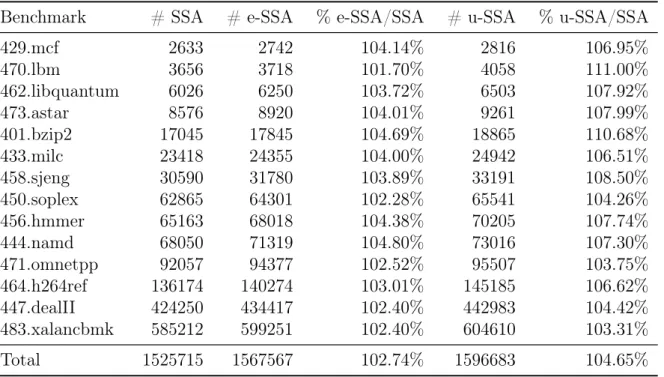
Figure 3.1 compares the u-SSA form with the SSA and e-SSA intermediate pro-gram representations. We use the notation v = • to denote a definition of variable v, and • =v to denote a use of it. Figure 3.1(b) shows the example program converted to the SSA format. Different definitions of variable u have been renamed, and a φ -function joins these definitions into a single name. The SSA form sparsifies a data-flow analysis that only extracts information from the definition sites of variables, such as constant propagation. Figure 3.1(c) shows the same program in e-SSA form. This time we have renamed variablev right after the conditional test where this variable is used. The e-SSA form serves data-flow analyses that acquire information from definition sites and conditional tests. Examples of these analyses include array bounds checking elimi-nation (Bodik et al. [2000]) and traditional implementations of range analyses (Gough and Klaeren [1994]; Patterson [1995]). Finally, Figure 3.1(d) shows our example in u-SSA form. The live range of variable v1 has been divided right after its use. This representation assists analyses that learn information from the way that variables are used, and propagate this information forwardly.
3.2. Experiments 19
v = • (v > 0)?
u = v + 10 u = •
• = u • = v
v = • (v > 0)?
u0 = v + 10 u1 = •
u2 = ϕ(u0, u1) • = u2
• = v
v0 = • (v0 > 0)?
v1 = v0∩ [-∞, 0]
u0 = v1 + 10
v2 = v0∩ [1, ∞]
u1 = •
u2 = ϕ(u0, u1)
v3 = ϕ(v1, v2)
• = u2
• = v2
v0 = • (v0 > 0)?
v1 = v0∩ [-∞, 0] u0 = v1 + 10
v4 = v1
v2 = v0∩ [1, ∞] u1 = •
u2 = ϕ(u0, u1) v3 = ϕ(v4, v2) • = u2 • = v2
(a) (b)
(c) (d)
Figure 3.1. (a) Example program. (b) SSA form [Cytron et al. [1991]]. (c) e-SSA form [Bodik et al. [2000]]. (d) u-SSA form.
20 Chapter 3. Live Range Splitting
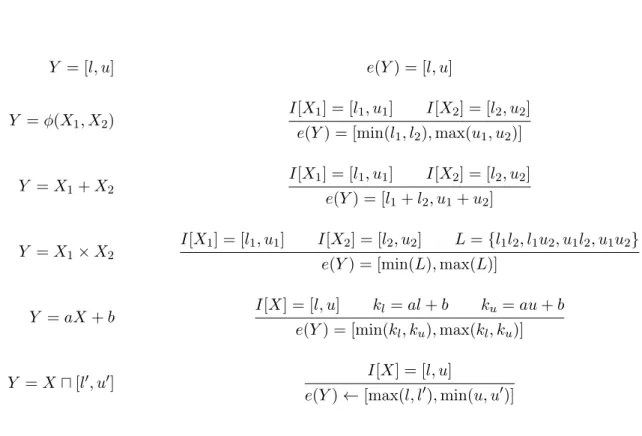
Benchmark # SSA # e-SSA % e-SSA/SSA # u-SSA % u-SSA/SSA
429.mcf 2633 2742 104.14% 2816 106.95%
470.lbm 3656 3718 101.70% 4058 111.00%
462.libquantum 6026 6250 103.72% 6503 107.92%
473.astar 8576 8920 104.01% 9261 107.99%
401.bzip2 17045 17845 104.69% 18865 110.68%
433.milc 23418 24355 104.00% 24942 106.51%
458.sjeng 30590 31780 103.89% 33191 108.50%
450.soplex 62865 64301 102.28% 65541 104.26%
456.hmmer 65163 68018 104.38% 70205 107.74%
444.namd 68050 71319 104.80% 73016 107.30%
471.omnetpp 92057 94377 102.52% 95507 103.75%
464.h264ref 136174 140274 103.01% 145185 106.62%
447.dealII 424250 434417 102.40% 442983 104.42%
483.xalancbmk 585212 599251 102.40% 604610 103.31%
Total 1525715 1567567 102.74% 1596683 104.65%
Table 3.1. Impact of the transformation to e-SSA and u-SSA in terms of program size. # SSA: number of instructions in the SSA form program. # e-SSA: number of instructions in the e-SSA form program. # u-e-SSA: number of instructions in the u-SSA form program.
3.2
Experiments
We have observed the actual impact of the transformation of programs to e-SSA and u-SSA forms. Table 3.1 shows the effect of the transformation in the programs of the SPEC CPU 2006 benchmarks. According to the table, we can observe that both representations lightly affect the number of instructions of the programs. From those benchmarks, we can see that e-SSA causes an average growth of 2.74% and a maximum growth of 4.8% of the program size, while u-SSA causes growths of 4.65% and 11,00% respectively. Those results, however, are not exclusive to that set of programs. We have similar results when we perform the same experiment on a set of benchmarks extracted from the LLVM test-suite infrastructure and from SPEC CPU 2006.
3.3. Conclusion 21
e-SSA u-SSA
1 1,05 1,1 1,15 1,2 1,25 1,3
Figure 3.2. Growth on the number of instructions in comparison with SSA representation.
instructions by more than 10% and that when this increment is higher than 15% it can be considered an outlier. The second box shows that the increment in the number of instructions is inferior to 10% in most of cases. However, in some cases it can reach up to 20%.
3.3
Conclusion
22 Chapter 3. Live Range Splitting
Chapter 4
Range Analysis
Most of the material in this chapter has been published in the paper "Speed and Pre-cision in Range Analysis" (Campos et al. [2012]). Here we expand that first discussion, with more examples and details.
4.1
Background
Following Gawlitza et al. [2009]’s notation, we shall be performing arithmetic operations over the complete lattice Z = Z∪ {−∞,+∞}, where the ordering is naturally given by −∞< . . . <−2<−1<0<1<2< . . .+∞. For any x >−∞ we define:
x+∞=∞, x6=−∞ x− ∞=−∞, x6= +∞
x× ∞=∞ if x >0 x× ∞=−∞ if x <0
0× ∞= 0 (−∞)× ∞= not defined
From the lattice Z we define the product lattice Z2
, which is defined as follows:
Z2
={∅} ∪ {[z1, z2]| z1, z2 ∈ Z, z1 ≤z2, −∞< z2}
This interval lattice is partially ordered by the subset relation, which we denote by "⊑". The meet operator "⊓" is defined by:
[a1, a2]⊓[b1, b2] =
[max(a1, b1),min(a2, b2)], if a1 ≤b1 ≤a2 orb1 ≤a1 ≤b2
∅, otherwise
The join operator, "⊔", is given by:
24 Chapter 4. Range Analysis
Y = [l, u] e(Y) = [l, u]
Y =φ(X1, X2) I[X1] = [l1, u1] I[X2] = [l2, u2]
e(Y) = [min(l1, l2),max(u1, u2)]
Y =X1+X2 I[X1] = [l1, u1] I[X2] = [l2, u2]
e(Y) = [l1+l2, u1+u2]
Y =X1×X2 I[X1] = [l1, u1] I[X2] = [l2, u2] L={l1l2, l1u2, u1l2, u1u2} e(Y) = [min(L),max(L)]
Y =aX+b I[X] = [l, u] kl=al+b ku=au+b
e(Y) = [min(kl, ku),max(kl, ku)]
Y =X⊓[l′, u′] I[X] = [l, u]
e(Y)←[max(l, l′),min(u, u′)]
Figure 4.1. A suite of constraints that produce an instance of the range analysis problem.
Given an interval ι = [l, u], we let ι↓ = l, and ι↑ = u. We let V be a set of
constraint variables, and I : V 7→ Z2
a mapping from these variables to intervals in
Z2
. Our objective is to solve a constraint system C, formed by constraints such as those seen in Figure 4.1(left). We let the φ-functions be as defined by Cytron et al. [1991]: they join different variable names into a single definition. Figure 4.1(right) defines a valuation functione on the interval domain. Armed with these concepts, we define the range analysis problem as follows:
Definition 4.2 Range Analysis Problem
Input: a set C of constraints ranging over a set V of variables.
Output: a mapping I such that, for any variable V ∈ V, e(V) = I[V].
rep-4.3. Our Design of a Range Analysis Algorithm 25
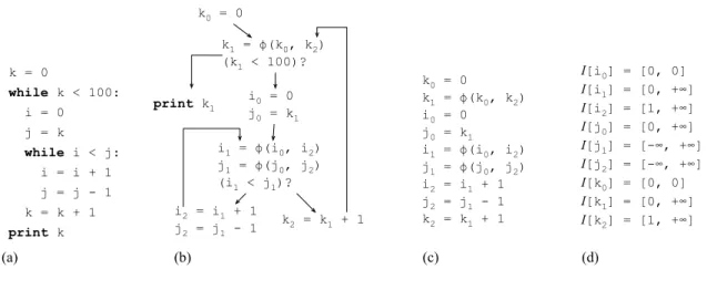
k = 0
while k < 100:
i = 0 j = k
while i < j:
i = i + 1 j = j - 1 k = k + 1
print k
k0 = 0
k1 = ϕ(k0, k2) (k1 < 100)?
i0 = 0 j0 = k1 i1 = ϕ(i0, i2) j1 = ϕ(j0, j2) (i1 < j1)?
k2 = k1 + 1 i2 = i1 + 1
j2 = j1 - 1
(a) (b) (c) (d)
k0 = 0
k1 = ϕ(k0, k2) i0 = 0
j0 = k1 i1 = ϕ(i0, i2) j1 = ϕ(j0, j2) i2 = i1 + 1 j2 = j1 - 1 k2 = k1 + 1
I[i0] = [0, 0] I[i1] = [0, +∞]
I[i2] = [1, +∞] I[j0] = [0, +∞] I[j1] = [-∞, +∞] I[j2] = [-∞, +∞] I[k0] = [0, 0] I[k1] = [0, +∞] I[k2] = [1, +∞]
print k1
Figure 4.2. (a) Example program. (b) Control Flow Graph in SSA form. (c) Constraints that we extract from the program. (d) Possible solution to the range analysis problem.
resentation we can not extract information from the conditional branches. As we will see shortly, we can improve this solution substantially by using a more sophisticated program representation – the e-SSA form – which gives us flow-sensitiveness.
Our analysis is not like classical abstract interpretation implemented in PAGAI by Henry et al. [2012], where the constraints are assigned to program points. Instead, we assign information to the variables, as a strategy to achieve sparsity in our analysis. Because SSA ensures that a variable is defined in a unique point of the program, the constraint assigned to a variable holds in every program points that the variable is alive. Thus, this association of constraints to variables is sound because we are using the SSA form and e-SSA, that also have all the properties of SSA.
4.3
Our Design of a Range Analysis Algorithm
In this section we explain the algorithm that we use to solve the range analysis prob-lem. This algorithm involves a number of steps. First, we convert the program to a suitable intermediate representation that makes it easier to extract constraints. From these constraints, we build a dependence graph that allows us to do range analysis sparsely. Finally, we solve the constraints applying different fix-point iterators on this dependence graph. Figure 4.3 gives a global view of this algorithm. Some of the steps in the algorithm are optional. They improve the precision of the range analysis, at the expense of a longer running time.
26 Chapter 4. Range Analysis
Path sensitive: e-SSA interprocedural:
formal = actual context sensitive: function inline Extract Constraints Build constraint graph Compute SCCs Sort topologically Remove control dep. edges Growth analysis Fix futures Narrowing analysis For each SCC in topological order Strongly Connected Components
Figure 4.3. Our implementation of range analysis. Rounded boxes are optional steps.
in Figure 4.2 is imprecise because we did not take conditional tests into considerations. Branches give us information about the ranges that some variables assume, but only at
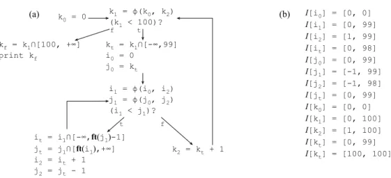
specificprogram points. For instance, given a test such as(k1 <100)?in Figure 4.2(b), we know thatI[k1]⊑[−∞,99] whenever the condition is true. In order to encode this information, we might split the live range of k1 right after the branching point; thus, creating two new variables, one at the path where the condition is true, and another where it is false. There is a program representation, introduced by Bodik et al. [2000], that performs this live range splitting: theExtended Static Single Assignment form, or e-SSA for short.
Given that the exact rules to convert a program to e-SSA form have never been explicitly stated in the literature, we describe our rules as follows. Let (v < c)? be a conditional test, and let lt and lf be labels in the program, such that lt is the target of the test if the condition is true, and lf is the target when the condition is false. We split the live range of v at any of these points if at least one of two conditions is true: (i) lf or lt dominate any use of v; (ii) there exist a use of v at the dominance frontier of lf or lt. For the notions of dominance and dominance-frontier, see [Aho et al., 2006, p.656]. To split the live range ofv atlf we insert at this program point a copy vf =v⊓[c,+∞], where vf is a fresh name. We then rename every use of v that is dominated by lf to vf. Dually, if we must split at lt, then we create at this point a copyvt=v⊓[−∞, c−1], and rename variables accordingly. If the conditional uses two variables, e.g., (v1 < v2)?, then we create intersections bound to futures. We insert, at lf, v1f = v1 ⊓[ft(v2),+∞], and v2f = v2⊓[−∞,ft(v1)]. Similarly, at lt we insert
4.3. Our Design of a Range Analysis Algorithm 27
k0 = 0 k1 = ϕ(k0, k2)
(k1 < 100)?
kt = k1∩[-∞,99]
i0 = 0
j0 = kt
i1 = ϕ(i0, i2) j1 = ϕ(j0, j2) (i1 < j1)?
k2 = kt + 1
it = i1∩[-∞,ft(j
1)-1]
jt = j1∩[ft(i
1),+∞]
i2 = it + 1
j2 = jt - 1
(b) I[i0] = [0, 0]
I[i1] = [0, 99]
I[i2] = [1, 99]
I[it] = [0, 98]
I[j0] = [0, 99]
I[j1] = [-1, 99]
I[j2] = [-1, 98]
I[jt] = [0, 99]
I[k0] = [0, 0]
I[k1] = [0, 100]
I[k2] = [1, 100]
I[kt] = [0, 99]
I[kt] = [100, 100]
(a)
kf = k1∩[100, +∞]
print kf
t f
f t
Figure 4.4. (a) The control flow graph from Figure 4.2(b) converted to standard e-SSA form. (b) A solution to the range analysis problem
We use the notation ft(v) to denote the future bounds of a variable. As we will show in Section 4.3.1, once the growth pattern of v is known, we can replace ft(v) by an actual value. After splitting the live ranges according to the rules stated above, we might have to insert φ-functions into the transformed program to re-convert it to SSA form. This last step avoids that two different names given to the same original variable be simultaneouslyaliveat the program code. A variablev is alive at a program point p if the program’s control flow graph contains a path fromp to a site where v is used, that does not go across any re-definition of v. Figure 4.4(a) shows our running example changed into standard e-SSA form. We have not created variable names forif and jf, because neitheri1 nor j1, the variables that have been renamed, are dominated by the target of the conditional’s else case. In this example, new φ-functions are not necessary: new variable names are not alive together with the original variables. The part (b) of this figure shows the solution that we get to this new program. The e-SSA form allows us to bind interval information directly to the live ranges of variables; thus, giving us the opportunity to solve range analysis sparsely. More traditional approaches, which we call dense analyses, bind interval information to pairs formed by variables and program points.
Extracting Constraints. Our implementation handles 18 different assembly instruc-tions. The constraints in Figure 4.1 show only a few examples. Instructions that we did not show include, for instance, the multiplicative operators div and modulus, the
bitwise operators and, or, xor and neg, the different types of shifts, and the logical
28 Chapter 4. Range Analysis
0 k0
k1 kt
k2
j0
j1
jt
j2
0 i0
i1
it i2
[-∞,99]
[-∞, ft(j
1)-1] [ft(i1), +∞]
+1 = −1 +1 ϕ ϕ ϕ
[100, +∞]
kf
Figure 4.5. The dependence graph that we build to the program in Figure 4.4.
is, given that numbers are internally represented in 2’s complement, the same imple-mentation of a constraint handles positive and negative numbers. However, there are instructions that require different constraints, depending on the input being signed or not. Examples include modulus and div. We also handle different kinds of type
conversion, e.g., converting 8-bit characters to 32-bit integers and vice-versa. In ad-dition to constraints that represent actual assembly instructions, we have constraints to representφ-functions, and intersections, as seen in Figure 4.1. The growth analysis that we will introduce in Section 4.3.1 require monotonic transfer functions. Many assembly operations, such as modulus or division, do not afford us this monotonic-ity. However, these non-monotonic instructions have conservative approximations, as shown by Warren [2002].
The Constraint Graph. The main data structure that we use to solve the range analysis problem is a variation of theprogram dependence graphof Ferrante et al. [1987]. For each constraint variable V we create a variable node Nv. For each constraint C we create a constraint node Nc. We add an edge from Nv to Nc if the name V is used in C. We add an edge from Nc to Nv if the constraint C defines the name V. Figure 4.5 shows the dependence graph that we build for the e-SSA form program given in Figure 4.4(a). If V is used by C as the input of a future, then the edge from Nv toNc represents what Ferrante et al. call a control dependence[Ferrante et al., 1987, p.323]. We use dashed lines to represent these edges. All the other edges denote data dependencies[Ferrante et al., 1987, p.322].
![Figure 3.1. (a) Example program. (b) SSA form [Cytron et al. [1991]]. (c) e-SSA form [Bodik et al](https://thumb-eu.123doks.com/thumbv2/123dok_br/15767033.129220/47.892.189.712.152.674/figure-example-program-ssa-form-cytron-ssa-bodik.webp)