Monopoly rights can reduce income big time

Monopoly Rights Can Reduce Income Big

Time

∗

Berthold Herrendorf

Universidad Carlos III de Madrid, University of Southampton, CEPR

Arilton Teixeira

Ibmec

February 26, 2003

Abstract

We study a two–sector version of the neoclassical growth model with coalitions of factor suppliers in the capital producing sectors. We show that if the coalitions have monopoly rights, then they block the adoption of the efficient technology. We also show that blocking leads to a decrease in the productivity of each capital producing sector and to an increase in the relative price of capital; as a result the capital stock and the production fall ineach sector. We finally show that the implied fall in the level of per–capita income can be large quantitatively.

Keywords: capital accumulation; monopoly rights; technology adoption; total factor productivity; vested interests.

JEL classification: EO0; EO4.

∗_{We are grateful to Edward Prescott and James Schmitz for their continuous help and encouragement}

and to Peter Klenow for sharing his price data with us. We have profited from comments and suggestions by Michele Boldrin, Juan Carlos Conesa, Antonia D´ıaz, Thomas Holmes, Juan Ruiz, Michele Tertilt, ´Akos Valentinyi, and the audiences of the European Forum in Maastricht, the Madrid Macro Seminar (Mad-Mac), the Thanksgiving Conference in Essex, and the University of Barcelona. Herrendorf acknowledges research funding from the Spanish Direcci´on General de Investigaci´on (Grant BEC2000-0170), from the European Union (Project 721, “New Approaches in the Study of Economic Fluctuations”), and from the Instituto Flores Lemus (Universidad Carlos III de Madrid).

†_{Address: Universidad Carlos III de Madrid, Departamento de Econom´ıa, Calle Madrid, 126, 28903}

Getafe (Madrid), Spain. Email: [email protected].

‡_{Address: Ibmec, Department of Economics, Av. Rio Branco, 108/12o. andar, Rio de Janeiro, RJ,}

1

Introduction

The per–capita income of the richest countries is many times larger than that of the

poor-est countries; see e.g. Parente and Prescott (1993), Hall and Jones (1999), and McGratten

and Schmitz (1999) for estimates. The objective of a successful theory of development

must be to explain the large income level difference without contradicting the growth

facts. Since differences in total factor productivity play an important role, a successful

theory needs to be also a theory of large cross-country differences in TFP [Klenow and

Rodriguez-Clare (1997) and Prescott (1998)]. One possible explanation is that a

sub-stantial part of the cross-country differences in TFP come from cross–country differences

in monopoly rights. If vested interest groups of factor suppliers are granted monopoly

rights, then they can block the adoption of the most efficient technologies or the best–

practice working arrangements. Blocking is optimal if it increases the real income of the

factor suppliers. Real–world examples of vested interest groups of factor suppliers are

brotherhoods, guilds, professional associations, trade unions, and the like, and there is

mounting evidence that they do block; see e.g. Mokyr (1990), McKinsey-Global-Institute

(1999), and Parente and Prescott (1999,2000).

Here we explore the quantitative implications of monopoly rights. Our main

innova-tion compared to the existing literature is to embed monopoly rights into the neoclassical

growth model with capital, where capital refers to tangible capital. The value added of

having capital is twofold. It allows us to study the interaction between technology

adop-tion and investment. In particular, we can study the conjecture of Parente and Prescott

(1999) that having capital magnifies the effect of monopoly rights on per–capita income.

Having capital also allows us to replicate the standard growth facts. Our theory of

devel-opment is therefore a theory of growth as well, which is desirable because develdevel-opment

and growth issues are intimately linked.

Our model economy is small and open. There are two final goods, which we call

services and manufacturing, and there are many intermediate goods. The service good

good is produced with the intermediate goods. The service good can only be consumed

and it is not tradable. The manufacturing good can be both consumed and invested and it

is tradable. The intermedidate goods are not tradable. In each intermediate good sector

there are insiders. The institutional arrangement is such that the insiders of a sector form

a coalition that chooses the marginal product of insider labor. We assume that the insiders

either do not have monopoly rights or they do have monopoly rights. If the insiders do

not have monopoly rights the outsiders can work in that sector without restrictions.

Outsider labor then is as productive as insider labor when the frontier technology is used,

implying that the insiders face unrestricted competition from the outsiders. If the insiders

of an intermediate good sector do have monopoly rights, then the outsiders can work in

that sector only with restrictions. Insider labor is then more productive than outsider

labor when the frontier technology is used, implying that the insiders face only restricted

competition from the outsiders.

We derive several analytical results. (i) When they have monopoly rights the coalitions

of insiders choose inefficient technologies; when they do not have monopoly rights, they

choose the frontier technology. (ii) The relative price of the domestic service good in terms

of the domestic manufacturing good is lower with monopoly rights; by construction, the

relative price of the domestic manufacturing good in terms of the foreign manufacturing

good is constant. (iii) All sectors’ capital stocks and the (economy–wide) per–capita

income are lower with monopoly rights. Results (ii) and (iii) imply that the relative price

of capital goods in terms of consumption goods be higher when per–capita income is lower.

Chari et al. (1996), Jovanovic and Rob (1997), Eaton and Kortum (2001), and Restuccia

and Urrutia (2001) report cross–country evidence consistent with this prediction. Results

(ii) and (iii) also imply that the relative price of non–tradable consumption goods in terms

of tradable capital goods be lower when per–capita income is lower and that the relative

price of tradable capital goods be unrelated to per–capita income. Hsieh and Klenow

(2002) report cross–country evidence consistent with these predictions.

each coalition is small relative to the aggregate economy, so it cannot affect any relative

price except for that of its intermediate good. Assuming that the demand for intermediate

goods is inelastic, the choice of an inefficient technology increases the relative price by

more than it decreases the marginal product of the insiders, so it increases the insiders’

real income. The extent to which they can increase their real income is limited by the

possibility that the outsiders enter the intermediate good sectors if the relative price

of intermediate goods has risen sufficiently. When this happens, the relative price is

determined by the requirement that the outsiders earn the same wage in the service sector

as in the intermediate good sector. Choosing yet more inefficient technologies then only

decreases the marginal product of the insiders, and so insider real income. Putting the

two arguments together, the equilibrium choice of technology is such that the outsiders

are just made indifferent between working in services and the intermediate good sector.

Why do monopoly rights reduce the price of services in terms of the manufacturing good?

The first point to note is that the equilibrium price of intermediate goods in terms of

domestic manufacturing goods must be equal to one. The second point is that we do not

have barriers to the international trade of the manufacturing good, so its price in terms

of the foreign manufacturing goods must equal one too. A decrease in the relative price of

the service good in terms of the domestic manufacturing good can then come only from

a decrease in the relative price of the domestic service good. This is possible because the

service good is not tradable.

We derive the following quantitative results. Given plausible parameter values,

mono-poly rights lead to a substantial decrease in the level of per–capita income. Specifically,

calibrating our model economy to the 1996 Benchmark Study of the Penn World Tables,

we find that monopoly rights can explain per–capita income differences of a factor 6.4.

This difference amounts to about 36 percent of the observed difference between the average

per–capita income levels of the ten percent richest and the ten percent poorest countries

in the 1996 Benchmark Study. Moreover, it is more than twice as big as the difference

Interestingly, we obtain such sizable income differences with a narrow concept of tangible

capital with capital shares that are empirically plausible [Gollin (2002)]. We conclude

from our quantitative findings that modeling the interaction between technology adoption

and investment is key to understanding the quantitative implications of monopoly rights.

Why do monopoly rights generate such substantial reductions in the per–capita income

of our model economy? The novelty here is that monopoly rights reduce the productions

ofall sectors, not just of the intermediate good sectors. The reductions in the intermediate

good productions, and thus in manufacturing, come from a direct and an indirect effect:

monopoly rights reduce productivity in the intermediate good sectors, which reduces

production and the capital stocks. The reduction in the service production comes from

an indirect effect: monopoly rights decrease the relative price of services in terms of capital

goods, making investment purchases more expensive for firms in the service sector. That

reduces the capital stock in the service sector. Capital therefore provides an amplification

mechanism that spreads the negative effects of monopoly rights to the competitive sectors.

2

Model Economy

2.1

Environment

There is a measure one of identical outsiders and measures one of identical insiders of type

i for all i ∈ [1,2]. All individuals are endowed with one unit of time in each period and with a positive capital stock in the first period. There are two final goods called x and

y and a continuum of intermediate goods called zj, j ∈[1,2]. x is a service good, which

can only be consumed, and y is a manufacturing good, which can be both consumed

and invested. The service good and the intermediate goods are non–tradable and the

manufacturing good is tradable. The economy is small in that it does not affect the world

market price of the tradable good.

prob-lem of the representative outsider is:

max

{xot, yot, kot+1}∞_t=0

∞

X

t=0

βtu(xot, yot) s.t. pxtxot+yot+kot+1 = (1 +rt−δ)kot+wot, (1)

xot, yot, kot+1 ≥0, ko0 >0 given.

The utility function has the standard functional form

u(x, y) = (x

α_y1−α₎1−ρ

1−ρ .

We have used the following notation. β ∈ (0,1) is the discount factor; the subscript o

stands for outsider; α ∈(0,1) is the expenditure share of xot; ρ ∈[0,∞) is the

intertem-poral elasticity of substitution; pxt is the price of xt in terms of the numeraire yt; kot+1

is the capital stock for period t+ 1 and kot is the installed capital stock held by the

representative outsider in period t; wot and rt are the outsider wage and the real rental

rate of installed capital, both expressed in terms of the numeraire yt; δ ∈ [0,1] is the

depreciation rate of installed capital. The problem of the representative insider of type i,

i∈[1,2], is similar:

max

{xit, yit, kit+1}∞t=0

∞

X

t=0

βtu(xit, yit) s.t. pxtxit+yit+kit+1 = (1 +rt−δ)kit+wit, (2)

xit, yit, kit+1 ≥0, ki0 >0 given.

Next we turn to the production side of the model economy. There is perfect

com-petition and free entry, so equilibrium profits will be zero. It is therefore without loss

of generality that we have omitted profits from the individuals’ problems above. The

representative firm in the service sector faces the following sequence of static problems:

max

xt, kxt, lxt

(pxtxt−rtkxt−wotlxt) s.t. xt=kxtθ (γ t

lxt)1−θ, xt, kxt, lxt ≥0, (3)

augmenting technical progress, andkxtandlxtare the inputs of capital and outsider labor.

The representative firm in the manufacturing sector faces the following sequence of static

problems:

max

yt, zyjt

yt−

Z 2

1

pzjtzyjtdj

s.t. yt=

Z 2

1

zyjt σ−1

σ dj

σ σ−1

, yt, zyjt ≥0, (4)

where pzjt is the price of intermediate good zjt in terms of the numeraire yt, zyjt is

the input of the j–th intermediate good, and σ ∈ (0,1) is the elasticity of substitution between any two intermediate goods. As in Parente and Prescott (1999), our results

require that the manufacturing sector’s demand for each intermediate good is inelastic

(σ < 1). An inelastic demand for each intermediate good can be obtained by grouping

goods appropriately (Volkswagen cars versus Mercedes cars or cars versus bicycles). The

representative firm in the j–th intermediate good sector faces the following sequence of

static problems:

max

zjt, kzjt, lzjot, lzjit

(pzjtzjt−rtkzjt−wotlzjot−wjtlzjit) (5)

s.t. zjt =kzjtθ [(1−ω)γ t_l

zjot+γτjtlzjit]1−θ, zjt, kzjt, lzjot, lzjit ≥0,

where wjt is the wage for insiders of sector j. The exogenous parameter ω ∈ [0,1) is a

measure of how strong the monopoly rights are: ω = 0 corresponds to “no monopoly

rights” and ω > 0 corresponds to “monopoly rights”. The value of τjt is determined in

period t−1 at the same time when all other decisions of period t−1 are taken. The insiders of sectorj then form a coalition that choosesτjt ∈[−∞, t] so as to maximize the

present value of their utility. The assumption that the highest possibleτjt equalstimplies

that the growth rates of the technological frontiers are the same in the intermediate good

sectors and in the service sector.

first alternative has outsiders and insiders produce with different capital stocks:

zjt =kzjotθ [(1−ω)γtlzjot]1−θ+kzjitθ (γτjtlzjit)1−θ.

This could be the case, for example, if the entry of outsiders happened through the entry

of new firms that hired only outsiders. We found that this alternative does not make

a difference for our results, so choosing our specification is merely a matter of carrying

a little less notation. The second alternative has the coalition choose not only its own

productivity but also that of the outsiders:

zjt =kzjtθ {γ

τjt_[(1−ω)l

zjot+lzjit]}1−θ.

This would be the case if the insiders had more monopoly power than in our specification.

We found that the BGP with monopoly rights then becomes indeterminate, so we prefer

our specification.

Trade takes place in sequential markets. In each period there are markets for both

final goods, for each intermediate good, for capital, for outsider labor, and for each type

of insider labor. Denoting aggregate variables by upper–case letters the market clearing

conditions are:

Xt=Xot+

Z 2

1

Xitdi, (6a)

Yt+Yt∗+ (1−δ)

Kot+

Z 2

1

Kitdi

= (Yot+Kot+1) +

Z 2

1

(Yit+Kit+1)di, (6b)

Zjt =Zyjt, (6c)

Kot+

Z 2

1

Kitdi=Kxt+

Z 2

1

Kzjtdj, (6d)

Lxt= 2−

Z 2

1

(Lzjot+Lzjit)dj. (6e)

The first two market clearing conditions require that the markets for final goods clear,

where Y∗

the markets for intermediate goods clear. The last two market clearing conditions require

that the factor markets clear.

Our model economy abstracts from borrowing between insiders and outsiders and

between domestic and foreign individuals. This is without loss of generality because

we will only consider balanced growth paths. Without borrowing and lending between

domestic and foreign individuals, international trade is balanced in each period: Yt∗ = 0.

So, in our model economy, the only implication of international trade is to fix the relative

price between domestic and foreign manufacturing goods at one.

2.2

Equilibrium

Our environment gives rise to a dynamic game. Since each coalition has strategic power

in its sector, care needs to be taken in defining the equilibrium. Since each coalition is

small compared to the rest of the economy, however, it does not have strategic power

on the aggregate. This will considerably simplify matters. We restrict our attention to

equilibria that have the following properties: they are symmetric with respect to each

type of individual and to the intermediate good sectors; they are recursive in that in each

period it is sufficient that the decision makers know the aggregate state and their own

state.

We start the equilibrium definition by specifying the relevant state variables. As

before, we denote the individual states by lower–case letters and aggregate states by

upper case letters. In periodtthe aggregate state variable is given by the aggregate capital

stock, the aggregate technology parameter, and the technology frontier: S ≡ (K,T, t). The states of the individuals and the coalition are given by the aggregate state plus the

relevant individual state: (S, ko) and (S, ki, τ). To avoid confusion, note that since we

look at a symmetric equilibrium, we have dropped the index indicating the intermediate

good sector, so the states T and τ are numbers, not vectors. We will also drop the time index

representative firms are static and straightforward to solve, so we do not repeat them

here. The problem of the representative outsider is dynamic. Using his value function,

vo, we can write it as:

vo(S, ko) = max xo, yo, k′o≥0

{u(xo, yo) +βvo(S′, ko′)} (7)

s.t. px(S)xo+yo+k′o = [1 +r(S)−δ]ko+wo(S), S′ =G(S),

where the aggregate law of motion is given by:

S′ =G(S) = (Gk, Gτ, G3)(S).

The solution to the outsider’s problem implies the policy function

(xo, yo, ko′) = (gxo, gyo, gko)(S, ko).

The problem of the representative insider differs from that of the representative outsider

in that the insider’s wage (in units of the numeraire) depends on the state of technology

in his sector:

vi(S, ki, τ) = max xi, yi, ki′≥0

{u(xi, yi) +βvi(S′, k′i, τ′)} (8)

s.t. px(S)xi+yi+k′i = [1 +r(S)−δ]ki+wi(S, τ),

S′ =G(S), τ′ =gτ c(S, ki, τ),

where gτ c is the policy function of the representative insider coalition. The solution to

the insider’s problem implies the policy function

The problem of the representative coalition is:

vc(S, ki, τ) = max τ′_∈(−∞,G

3(S)]

{u(xi, yi) +βvc(S′, ki′, τ′)} (9)

s.t. S′ =G(S), (xi, yi, k′i) = (gxi, gyi, gki)(S, ki, τ).

A solution to the problem of the representative coalition implies the policy function

τ′ =gτ c(S, ki, τ).

Definition 1 (Equilibrium) An equilibrium is

(i) price functions (px, pz, wo, r)(S), wi(S, τ);

(ii) allocation functions for the three types of firms,(x, kx, lx)(S),(y, zy)(S), (z, kz, lzo, lzi)

(S, τ),

(iii) aggregate laws of motion S′ _{= (G}

k, Gτ, G3)(S);

(iv) value functions vo(S, ko), vi(S, ki, τ), vc(S, ki, τ);

(v) policy functions k_o′ =gko(S, ko), ki′ =gki(S, ki, τ), τ′ =gτ c(S, ki, τ),

such that:

1) given the realizations of prices, the firms’ allocations solve their problems;

2) the value functionsvo, vi, vc satisfy the Bellman equations as stated in (7), (8), (9);

3) the problems of the representative outsider, the insider, and the coalition, (7), (8),

and (9), are solved by their policy functions;

4) the policy functions are consistent with the laws of motion:

Gk(S) = gko(S, ko) +gki(S, ki,T), Gτ(S) = gτ c(S, K,T);

3

Analytical Results

In this section, we study the BGPs of the model economy without and with monopoly

rights; recall that these two cases correspond to ω = 0 and ω > 0. We will show that

all real variables ascend parallel balanced growth paths but that their levels are higher

without monopoly rights. For the formal analysis we need to ensure that the growth rates

of the technological frontiers are not too large relative to the discount factor (otherwise the

individual objective functions would become infinite) and that a BGP without monopoly

rights exists. The next assumptions serve this purpose.

Assumption 1 β˜≡βγ ∈(0,1).

Assumption 2

0<(1−α)(1−θ) + [(1−α)θ+δ+γ−1)] βθ

γρ_{−β(1−δ)} <

1 2.

Proposition 1 (BGP Without Monopoly Rights) Suppose thatω = 0 and that

As-sumptions 1 and 2 hold. Then there is a unique BGP equilibrium in which the most

efficient technology is adopted. Along this BGP equilibrium, pxt = 1; the technology

parameter, the capital stocks, the productions of all goods grow at rate γ−1.

Proof. See Appendix B.

Note that the BGP equilibrium is only unique subject to the constraint that the best

technology be adopted. In fact, any technology choice is an equilibrium because the

insiders can work in services at the maximum wage that they may earn in intermediate

goods, so choosing inefficient technologies has no consequences when all insiders work in

services. These equilibria are not interesting or plausible, so we will not consider them.

To ensure the existence of a BGP equilibrium without monopoly rights, we need two

Assumption 3

αβθ(γ+δ−1)(2−ω)<[α−(1−α)(1−ω)][γρ−β(1−δ)], (10a) 2αβθ(γ+δ−1)>(2α−1)[γρ−β(1−δ)]. (10b)

Proposition 2 (BGP With Monopoly Rights) Suppose ω > 0 and Assumptions 1

and 3 hold. Then there is a unique BGP equilibrium. Along the BGP equilibrium,

inef-ficient technologies are used: t−τt >0 and constant; pxt <1; the capital stocks and the

productions of all goods grow at rate γ −1; the outsiders work only in the service sector and the insiders work only in their intermediate good sector; the capital stocks and the

quantities of all goods are smaller than without monopoly rights.

Proof. See Appendix B.

It is optimal for the representative insider coalition to choose inefficient technologies

because this increases the insiders’ real wage. We show in Appendix B that the highest

insider wage is obtained exactly when the technology is so inefficient that the outsider

are just indifferent between working in services and in the intermediate good sector. If

efficiency increased relative to that value, then the insider wage would fall. The reason

is that the demand for each intermediate good is inelastic here, so the decreases in the

relative price would dominate the increase in the marginal insider productivity. If

effi-ciency decreased relative to the above value, then the wage would fall too. The reason

now is that the outsiders would remain indifferent, so the relative price would remain the

same and a decrease in the marginal insider productivity would be the only effect on the

insider wage.

An important implication of Proposition 2 is that having monopoly rights in the

intermediate good sectors reduces the capital stocks of all sectors. The reason can most

easily be seen by noting that along a BGP where the outsiders work only in the service

reduce to

θ

γτt Kzt

1−θ

=pxtθ

γt

Kxt

1−θ

= γ

ρ

β −1 +δ.

So, the direct effect of monopoly rights is to decrease productivity in the intermediate

good sectors, τt < t. This decreases the capital stocks in the intermediate good sectors.

The indirect effect of monopoly rights is to decrease the relative price of services, pxt =

(1−ω)1−θ _{< 1. This decreases the capital stock of the service sector. In other words,}

capital provides an amplification mechanism by which monopoly rights in one part of the

economy affect the part of the economy that is free of them. In the next section, we will

see that this amplification mechanism generates big reductions in per–capita income.

Propositions 1 and 2 imply the qualitative prediction that the relative price of capital

be higher in countries with lower per–capita incomes. This is consistent with the evidence

reported by, among others, Chari et al. (1996), Jovanovic and Rob (1997), Eaton and

Kortum (2001), and Restuccia and Urrutia (2001). In our model economy, the difference

in the relative prices of capital is entirely due to a lower relative price of non–tradable

service goods when monopoly rights are effective. The price of domestic capital goods

in terms of foreign capital goods is unaffected by monopoly rights, as capital goods are

assumed to be tradable across regimes. These featurs are qualitatively consistent with the

evidence reported by Hsieh and Klenow (2002) that, across countries, per–capita incomes

are positively correlated with the price of non–tradables in terms of capital goods whereas

they are uncorrelated with the price of domestic capital goods in terms of foreign (US,

that is) capital goods.

4

Quantitative Results

In this section, we explore by how much monopoly rights reduce the productivity in the

capital–producing sectors, the per–capita capital stocks, and per–capita income.1 _We

choose standard values for β, γ, δ, and θ. Recall that σ < 1 is also assumed, but we

do not need a specific value for σ. In particular, we choose β = 0.96, implying a net

real rate of return on capital of about 4 percent. We choose γ = 1.02, implying that the

technological frontier grows at 2 percent. This is about the long–run growth rate of the

US economy where many of the inventions and innovations that can be adopted by other

countries take place. We choose δ = 0.08, which is an upper bound on the reasonable

choices because useful lives are likely to be larger in developing countries than in the US.

This choice goes against us because a largerδ makes capital accumulation less important.

We chooseθ= 0.4, which implies a capital share of forty percent. There is a debate about

the right choice of θ for developing countries [see for example Boldrin and Jones (2002)

and Gollin (2002)]. We therefore explore our model economy also forθ ∈[0.3,0.45]. Note that we have imposed all sectors to have equal capital shares. We will need to evaluate

how reasonable that assumption is (if we knew that it was for the OECD countries or the

US, we could invoke the usual assumption that technology is uniform across the world).

To calibrate the rest of the parameters of the model economy, we use the 1996

Bench-mark Study of the Penn World Tables. This benchBench-mark study is unusually large in that it

documents detailed price and quantity data for 115 countries. We start by identifying the

ten percent countries with the highest per–capita incomes and the ten percent countries

with the lowest per–capita incomes in the sample (both measured in ppp–adjusted

inter-national prices). We find that the average per–capita income of the richest ten percent is

by a factor 17.73 larger than that of the poorest ten percent. Next, we calibrate α and

ω. We interpret α to be the expenditure share of non–tradable consumption goods in

total consumption expenditure measured in domestic currency. We find that across the

ten percent richest and poorest countries the average α equals 0.65. To calibrate ω, we

note that in the model economy with monopoly rights, ω determines the relative price

of services in terms of manufacturing goods: pxt = (1−ω)1−θ. In the model economy

without monopoly rights, this relative price equals one: pxt = 1. We compute the average

relative prices for both groups and obtain that the ratio of the average relative prices in

poorest countries correspond to our model economy with monopoly rights and the ten

percent richest countries correspond to our model economy without monopoly rights and

maintaining θ = 0.4, we obtain ω = 0.0364.

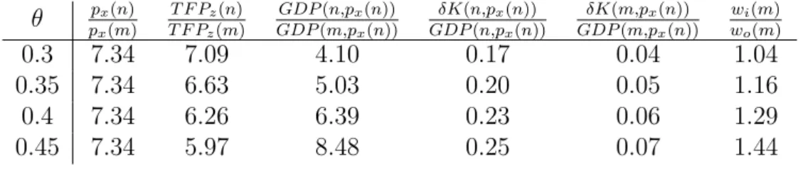
Table 1: Quantitative results (“m” for “monopoly rights”, “n” for “no monopoly rights”)

θ px(n)

px(m)

T F Pz(n)

T F Pz(m)

GDP(n,px(n))

GDP(m,px(n))

δK(n,px(n))

GDP(n,px(n))

δK(m,px(n))

GDP(m,px(n))

wi(m)

wo(m)

0.3 7.34 7.09 4.10 0.17 0.04 1.04 0.35 7.34 6.63 5.03 0.20 0.05 1.16 0.4 7.34 6.26 6.39 0.23 0.06 1.29 0.45 7.34 5.97 8.48 0.25 0.07 1.44

The quantitative results are summarized in Table 1. The first column shows that the

relative price difference is 7.34, as we calibrated it to be. The next column lists the ratios

of TFP in the intermediate good sector with and without monopoly rights, indicated by

the arguments “m” and “n”. In short, TFP in the intermediate good sectors is at least

six times higher without monopoly rights than with monopoly rights. The third column

lists the ratios of the per–capita incomes with and without monopoly rights evaluated at

international prices, so, for example, GDP(m, px(n)) = px(n)X(m) +Y(m). Note that

here we equate international prices with the relative prices without monopoly rights. This

is justified approximately (international prices are very close to prices in Belgium, which

is the 12–th richest country in our sample). We can see that monopoly rights reduce

the level of per–capita income by between a factor of four and a factor of eight. For our

calibrationθ= 0.4, the result is 6.39. The fourth and the fifth columns list the investment

shares in total output without monopoly rights and with monopoly rights, evaluated at

international prices. So, for example,

δK(m, px(n))

GDP(m, px(n))

= δpx(n)K(m)

px(n)X(m) +Y(m)

.

The predicted effect that of monopoly rights on the investment share is broadly consistent

22 percent and the ten percent poorest of 9.65 percent (both measured in ppp–adjusted

international prices). The last column lists the insider wage premium with monopoly

rights.

5

Conclusion

We have explored the implications of monopoly rights which put coalitions of insiders

into the position to resist the adoption of efficient technologies. Our innovation is to

have done so within the neoclassical growth model with tangible capital. We have found

that modeling explicitly the interaction between such monopoly rights and investment

magnifies the detrimental consequences of monopoly rights on the per–capita income level.

Specifically, we have demonstrated that reductions in the per–capita income level of more

than a factor of 6 are possible for reasonable parameter choices. This order of magnitude

is more than twice as large than that reported by Parente and Prescott (1999) for a

model without capital accumulation. The mechanism behind our large income reductions

is that monopoly rights in the capital–producing sector not only reduce productivity

and investment there, but they also increase the relative price of capital and so reduce

investment in the rest of the economy.

Our paper is placed within the branch of the development literature that seeks to

explain the observed differences in cross-country per capita incomes under the assumption

that the most productive technology is freely available once it is invented. The most

closely related papers to our’s are Holmes and Schmitz (1995), Parente and Prescott

(1999,2000), and Herrendorf and Teixeira (2002), who study the implications of monopoly

rights but abstract from capital accumulation. Further contributions to this literature

study different aspects: Mankiw et al. (1992) emphasize the role of intangible capital;

Chari et al. (1996), Jovanovic and Rob (1997), Eaton and Kortum (2001), and Restuccia

and Urrutia (2001)emphasize the role of policy distortions that increase the relative price

Zilibotti (2001) emphasize the role of skill mismatch. We view intangible capital, policy

distortions, home production, and skill mismatch as alternative explanations of TFP

differences that are complementary to our’s. Our results suggest, however, that monopoly

rights are a key part of the story.

References

Acemoglu, Daron and Fabrizio Zilibotti, “Productivity Differences,” Quarterly

Journal of Economics, 2001,115, 563–606.

Boldrin, Michele and Larry Jones, “Mortality, Fertility, and Savings in a Malthusian

Economy,” Manuscript, University of Minnesota 2002.

Chari, Varadarajan V., Patrick J. Kehoe, and Ellen R. McGrattan, “The

Poverty of Nations: a Quantitative Exploration,” Staff Report 204, Federal Reserve

Bank of Minneapolis, Research Department 1996.

Eaton, Jonathan and Samuel Kortum, “Trade in Capital Goods,” European

Eco-nomic Review, 2001,45, 1195–1235.

Gollin, Douglas, “Getting Income Shares Right,” Journal of Political Economy, 2002,

110, 458–474.

Hall, Robert and Charles I. Jones, “Why Do Some Countries Produce So Much

More Output Per Worker Than Others?,”Quarterly Journal of Economics, 1999,114,

83–116.

Herrendorf, Berthold and Arilton Teixeira, “How Trade Policy Affects Technology

Adoption and Productivity,” Discussion Paper 3486, CEPR 2002.

Holmes, Thomas J. and James A. Schmitz, “Resistance to New Technology and

Trade Between Areas,” Federal Reserve Bank of Minneapolis Quarterly Review, 1995,

Hsieh, Chang-Tai and Peter J. Klenow, “Relative Prices and Relative Prosperity,”

Manuscript, Federal Reserve Bank of Minneapolis 2002.

Jovanovic, Boyan and Rafael Rob, “Solow vs. Solow: Machine Prices and

Develop-ment,” Working Paper 5871, NBER 1997.

Klenow, Peter J. and Andres Rodriguez-Clare, “The Neoclassical Revival in

Growth Economics: Has It Gone Too Far?,” in “NBER Macroeconomics Annual,”

Cambridge, MA: MIT Press, 1997, pp. 73–103.

Mankiw, Gregory N., David Romer, and David N. Weil, “A Contribution to the

Empirics of Economic Growth,”Quarterly Journal of Economics, 1992, 112, 407–437.

McGratten, Ellen R. and James A. Schmitz, “Explaining Cross-Country Income

Differences,” in John B. Taylor and Michael Woodford, eds., Handbook of

Macroeco-nomics, Amsterdam: North Holland, 1999.

McKinsey-Global-Institute,Unlocking Economic Growth in Russia, McKinsey & Co.,

1999.

Mokyr, Joel, The Lever of Riches: Technological Creativity and Economic Progress,

Oxford University Press, 1990.

Parente, Stephen L. and Edward C. Prescott, “Changes in the Wealth of Nations,”

Federal Reserve Bank of Minneapolis Quarterly Review, 1993,17, 3–16.

and , “Monopoly Rights: a Barrier to Riches,”American Economic Review,

1999, 89, 1216–33.

and , Barriers to Riches, Cambridge, MA: MIT Press, 2000.

, Richard Rogerson, and Randall Wright, “Homework in Development

Eco-nomics: Household Production and the Wealth of Nations,”Journal of Political

Prescott, Edward C., “Needed: A Theory of Total Factor Productivity,” International

Economic Review, 1998,39, 525–52.

Restuccia, Diego and Carlos Urrutia, “Relative Prices and Investment Rates,”

Jour-nal of Monetary Economics, 2001, 47, 93–121.

Stokey, Nancy L. and Robert E. Lucas,Recursive Methods in Economic Dynamics,

Appendix A: First–order Conditions

We start with the individuals. The first–order conditions to problem (1) of the

represen-tative outsider are:

pxtxot =α[(1 +rt−δ)kot+wot−kot+1], (11a)

yot = (1−α)[(1 +rt−δ)kot+wot−kot+1], (11b)

(xot)α(1−ρ)

(yot)ρ+α(1−ρ)

=β(1 +rt+1−δ)

(xot+1)α(1−ρ)

(yot+1)ρ+α(1−ρ)

. (11c)

The first–order conditions to problem (2) of the representative insider are:

pxtxit =α[(1 +rt−δ)kit+wit−kit+1], (11d)

yit = (1−α)[(1 +rt−δ)kit+wit−kit+1], (11e)

(xit)α(1−ρ)

(yit)ρ+α(1−ρ)

=β(1 +rt+1−δ)

(xit+1)α(1−ρ)

(yit+1)ρ+α(1−ρ)

. (11f)

We continue with the firms. The first–order conditions to problem (3) of the

repre-sentative firm in the service sector are:

rt=pxtθkθxt−1(γ t

lxt)1−θ, (12a)

wot=pxt(1−θ)kxtθ γ

t(1−θ)_l−θ

xt. (12b)

The first–order conditions to problem (4) of the representative firm in the intermediate

good sector j imply the demand functions for intermediate goods j:

zyjt =

yt

pσ zjt

. (12c)

Imposing zero profits, in addition, gives:

1 =

Z 2

1

The first–order conditions to the problem (5) of the representative firm in the intermediate

good sector j, are:

rt =pzjtθkzjtθ−1(ωγ t

lzjot+γτitlzjit)1−θ, (12e)

wjt =pzjt(1−θ)kθzjtγ

τjt_(ωγt_l

zjot+γτjtlzjit)−θ, (12f)

wot ≥ωγt−τjtwjt. (12g)

Appendix B: Proofs

Proof of Proposition of 1

We start the proof by showing that there is a unique value function and a unique policy

function for the outsiders. (We omit the proof for the insiders because it is analogous.)

To this end, transform the relevant variables by deflating them by their postulated growth

rates along a balanced growth path:

˜

Tt ≡ Tt−t, x˜ot ≡

xot

γt, y˜ot≡

yot

γt, k˜ot ≡

kot

γt, K˜xt ≡

Kxt

γt , K˜zt ≡

Kzt

γt , K˜t ≡

Kt

γt.

The indirect period–t utility of the representative outsider can then be written as:

uo(˜kot,˜kot+1) = ˜βt

Φo[wot+ (1 +rt−δ)˜kot−γk˜ot+1]1−ρ

pα_xt(1−ρ) ,

where Φo ≡αα(1−ρ)(1−α)α(1−ρ). Using this, the Bellman equation for the representative

outsider can be rewritten as

˜

vo( ˜S,k˜o) = max

0≤˜k′o≤γ−1[wo+(1+r−δ)˜ko] n

uo(˜ko,˜ko′) + ˜βv˜o( ˜S′,k˜′o)

o

s.t. ˜S′ =G( ˜S).

Since there are decreasing marginal returns to capital and positive depreciation, there

is some maximal sustainable capital stock, which we call ¯k. Define the set of possible

the feasibility constraints as Γ : X →X by Γ(˜ko)≡ [0, γ−1{wo+ (1 +r−δ)˜ko}]. X and

Γ so defined satisfy the assumptions of Theorems 4.6, 4.8, and 4.11 of Stokey and Lucas

(1989), so there exists a unique value function and a unique policy function.

We continue by noting that the problem of the representative insider coalition is trivial

for ω = 0. If they do not adopt the most efficient technology, then the insider marginal

product in the intermediate good sector is strictly smaller than that of the outsiders. If

they do adopt the most efficient technology, then the insider marginal product in the

intermediate good sector is the same as that of the outsiders. Thus, the coalition cannot

improve upon adopting the most efficient technology. However, it is indifferent between all

technology choices. The reason is that if it does not adopt the most efficient technology,

then the insiders will work in services where they earn the same wage as the outsiders do

in services and manufacturing.

The next part of the proof is to show market clearing. We start by noting that

equalization of the wages and the real interest rates implies that the capital–labor ratios

are equalized, which, in turn, implies thatpxt= 1. This together with the Euler equations

(11c) and (11f) gives that along the BGP, the capital–labor ratio is given by:

˜

Kxt

Lxt

= K˜zt

Lzt

=

βθ γρ_{−β(1−δ)}

₁−1θ

. (13)

Using that ˜Kxt = ˜Kt−K˜zt and that ˜Lxt = 2−L˜zt, we also have

˜

Kt

2 =

βθ γρ_{−β(1−δ)}

₁−1θ

. (14)

Walras law implies that we only need to prove market clearing for the y–sector. The

supply of consumption manufacturing goods is given by:

˜

Kzt

Lzt

!θ

The demand for consumption manufacturing goods is

(1−α)







(1−θ) pxt

˜

Kxt

Lxt θ

+ K˜zt

Lzt θ!

+



1 +θ

˜

Kzt

Lzt

!θ−1

−δ−γ 

K˜t





 .

Substituting equations (13) and (14) into this equation and rearranging, we find:

Lzt

2 = (1−α)(1−θ) + [(1−α)θ+δ+γ−1)]

βθ

γρ_{−β(1−δ)} (15)

Assumption 2 ensures that this condition is satisfied for a unique Lzt∈(0,1).

The final part of the proof is to show the existence of a unique BGP. This follows

immediately from Theorem 4.6 of Stokey and Lucas (1989). Along the BGP, ˜K_x′ = ˜Kx

and ˜Kz′ = ˜Kz, so the two capital stocks grow at rate γ. Given that from the previous

proposition τtalso grows at rateγ, it follows that the quantities of all goods grow at rate

γ too.

Proof of Proposition 2

The first part of the proof is to show that there is a value function and a policy function

to the problems of the representative outsider and the representative insider. This part

of the proof is exactly the same with and without monopoly rights, so it is omitted here.

The second part of the proof is to show market clearing under the assumption that

the insiders work in their intermediate good sector and τt is such that the outsiders are

just indifferent between working in services and in their intermediate good sector. So,

the real returns on capital and on outsider labor need to be equalized across sectors:2

pxtK˜xtθ = ˜K θ

zt(1−ω)γ(

τt−t)(−θ)_{, (16a)}

pxtK˜xtθ−1 = ˜K θ−1 zt γ(

τt−t)(1−θ)_{, (16b)}

2_{Tildes again denote variables deflated byγ}t

implying

˜

Kxt

˜

Kzt

= (1−ω)γt−τt_{. (17)}

Putting this equation back into (16b), we obtain:

pxt= (1−ω)1−θ. (18)

Comparing this relative price with the previous one, we can see that the relative price of

services is smaller with than without monopoly rights. Using (17), (18), and the BGP

conditions that the marginal products of the capital stocks in terms of the z good are

given by γρβ−1−1 +δ, we get the two BGP capital stocks:

˜

Kxt= (1−ω)

βθ γρ_{−β(1−δ)}

₁−1θ

, (19a)

˜

Kzt =γτt−t

βθ γρ_{−β(1−δ)}

₁−1θ

. (19b)

Comparing these two expressions with those in (13), we can see that both capital stocks

are smaller than without monopoly rights. Given that productivity in the intermediate

good sector is also smaller (compare the previous proposition), this implies that the levels

of the per capita productions of the two goods are smaller too.

Due to Walras law, it is enough to prove market clearing for the y–sector. In period

t, the supply of manufacturing goods equals the total production plus the capital stock

after depreciation minus the capital stock for next period. Along a BGP with growth

rate γ, this is given by

˜

Kztθγ(

τt−t)(1−θ)_{+ (1−δ−γ) ˜K}

t.

In periodt, the representative outsider and the representative insider spend a share 1−αof their disposable income on the manufacturing good. Using that the wage of the outsiders

that from (19)

˜

Kt= (1 + (1−ω)γt−τt) ˜Kzt,

we obtain the consumption demand for manufacturing goods in period t:

(1−α)n[1 + (1−ω)γt−τt_{](1−θ) ˜K}θ

ztγ(

τt−t)(1−θ)_+θK˜θ−1

zt γ(

τt−t)(1−θ)_K˜

t+ (1−δ−γ) ˜Kt

o ,

where we have used the fact that in equilibrium Yt = Zt. Then, equalize supply and

demand and rearrange so as to find that the market for the manufacturing goods clears

if and only if

αβθ(γ+δ−1)(1 + (1−ω)γt−τt_{) = [α−(1−α)(1−ω)γ}t−τt_][γρ_{−β(1−δ)]. (20)}

Condition (10a) from Assumption 3 in the text ensures that the left–hand side is smaller

than the right–hand side when τt = t; Condition (10b) from Assumption 3 in the text

ensures that the left–hand side is larger than the right–hand side when τt is such that

(1−ω)γt−τt _{= 1. Thus, theτ}

tthat clears the market satisfies (1−ω)< γτt−t, implying that

the insiders will strictly prefer to work in the intermediate good sector. The uniqueness

ofτtfollows because both sides (20) change monotonically and in opposite directions with

τt.

The third part of the proof is to show that choosing τt such that the outsiders are

just indifferent is the unique equilibrium strategy for the representative insider coalition.

Substituting (12a) into (12b) and (12e) and (12f), we obtain the reduced forms for the

wages:

wot= (1−θ)p 1 1−θ xt

θ rt

θ

1−θ

γt, (21a)

wit = (1−θ)p 1 1−θ zt

θ rt

θ

1−θ

If the outsiders work in the intermediate good sector, then they can earn:

(1−θ)p

1 1−θ zt θ rt θ

1−θ

(1−ω)γt. (21c)

If the outsiders are indifferent, then the coalition wants to chooseτtas large as possible.

This follows because equalizing (21a) and (21c) implies

pzt =

pxt

(1−ω)1−θ.

In other words, the relative price is given to the coalition when the outsiders are

indif-ferent. Call

¯τt the largest such τt. Recall that we showed in the market clearing part of the proof above that

¯τt < t if the outsiders are indifferent. Moreover, we showed that

γ¯τt−t>1−ω, so we know that for τt>

¯τt, the insiders still prefer manufacturing and the outsiders now prefer services. To solve for the insider wage in this case, combine (12c)

with the production function from (5):

K_ztθγτt(1−θ) _=Y

tp−ztσ,

implying that

pzt =

Y 1 σ t K θ σ ztγ

τt(1−θ)

σ

. (22)

Combining this with (12e), we find:

Kzt=

Ytθσ

rσ

tγτt(1−θ)(1−σ)

_θ+σ(11_−θ)

. (23)

Substituting this expression back into (22) gives the relative price in terms of τt and of

variables that are exogenous to the coalition:

pzt = [θ−θYt1−θr θ tγ−

Finally, the insider wage results after substituting (23) and (24) into (21b):

wit = (1−θ)[θθ(σ−1)Ytr θ(1−σ)

t ]

1 θ+σ(1−θ)_γ−

(1−θ)(1−σ) θ+σ(1−θ) τt

. (25)

The assumption that σ < 1 implies that the insider wage increases when τt ∈ (τt, t]

decreases. So for τt∈[τt, t] it is optimal to chooseτt=τt.

The last part of the proof is to show that no other equilibrium than the one just

characterized can exist. Suppose that ˜τt > τt is part of an equilibrium. First, if the

insiders preferred to work in their intermediate good sector and the outsiders preferred to

work in services, then the insiders can increase their wage by decreasingτt; compare (25).

Second, if the insiders preferred to work in their services and the outsiders preferred to

work in intermediate goods, then we would have

γ˜τt−t_{< p}

1 1−θ

xt <1−ω.

The first inequality means that the production in the intermediate good sector is more

efficient than before, the second inequality means that the service good is cheaper than

before. That is inconsistent with market clearing. Third, if the insiders were indifferent

now, then there would be two subcases. If the outsiders worked only in the intermediate

good sector, then the insider could increase their wage by lowering ˜τt. If the outsiders

worked only in services, then

1−ω < γτ˜t−t_=p

1 1−θ xt .

Thus, the relative price of services is larger than before. This again is inconsistent with