www.biogeosciences.net/11/2991/2014/ doi:10.5194/bg-11-2991-2014
© Author(s) 2014. CC Attribution 3.0 License.
Can current moisture responses predict soil CO
2
efflux under
altered precipitation regimes? A synthesis of manipulation
experiments
S. Vicca1, M. Bahn2, M. Estiarte3,4, E. E. van Loon5, R. Vargas6, G. Alberti7,8, P. Ambus9, M. A. Arain10, C. Beier9,11, L. P. Bentley12, W. Borken13, N. Buchmann14, S. L. Collins15, G. de Dato16, J. S. Dukes17,18,19, C. Escolar20, P. Fay21, G. Guidolotti16, P. J. Hanson22, A. Kahmen23, G. Kröel-Dulay24, T. Ladreiter-Knauss2, K. S. Larsen9,
E. Lellei-Kovacs24, E. Lebrija-Trejos25, F. T. Maestre20, S. Marhan26, M. Marshall27, P. Meir28,29, Y. Miao30, J. Muhr31, P. A. Niklaus32, R. Ogaya3,4, J. Peñuelas3,4, C. Poll26, L. E. Rustad33, K. Savage34, A. Schindlbacher35, I. K. Schmidt36, A. R. Smith27,37, E. D. Sotta38, V. Suseela17,39, A. Tietema5, N. van Gestel40, O. van Straaten41, S. Wan30, U. Weber42, and I. A. Janssens1
1Research Group of Plant and Vegetation Ecology, Department of Biology, University of Antwerp, Universiteitsplein 1, 2610
Wilrijk, Belgium
2Institute of Ecology, University of Innsbruck, Sternwartestr. 15, 6020 Innsbruck, Austria
3CSIC, Global Ecology Unit, CREAF-CEAB-UAB, Cerdanyola del Vallés 08913, Catalonia, Spain 4CREAF, Cerdanyola del Vallés 08193, Catalonia, Spain
5Institute for Biodiversity and Ecosystem Dynamics, University of Amsterdam, the Netherlands
6Department of Plant and Soil Sciences, Delaware Environmental Institute, University of Delaware, Newark, DE, USA 7University of Udine, via delle Scienze 206, Udine, Italy
8MOUNTFOR Project Centre, European Forest Institute, Via E. Mach 1, San Michele all’Adige (Trento), Italy
9Department of Chemical and Biochemical Engineering, Technical University of Denmark, 2800 Kgs. Lyngby, Denmark 10McMaster Center for Climate Change and School of Geography and Earth Sciences, McMaster University, Hamilton,
Ontario, Canada
11NIVA – Norwegian Institute for Water Research, Gaustadalléen 21, 0349 Oslo, Norway 12Department of Biological Sciences, Texas Tech University, Lubbock, TX 79409, USA 13Soil Ecology, University Bayreuth, Dr.-Hans-Frisch-Str. 1–3, 95448 Bayreuth, Germany 14Department of Environmental Systems Science, ETH Zurich, Zurich, Switzerland 15Department of Biology, University of New Mexico, Albuquerque, NM 87131, USA
16Department for Innovation in Biological, Agro-food and Forest systems, University of Tuscia, Viterbo, Italy
17Department of Forestry and Natural Resources, Purdue University, 715 West State Street, West Lafayette, IN 47907-2061,
USA
18Department of Biology, University of Massachusetts, Boston, MA 02125, USA 19Department of Biological Sciences, Purdue University, West Lafayette, IN 47907, USA
20Área de Biodiversidad y Conservación, Departamento de Biología y Geología, Escuela Superior de Ciencias
Experimentales y Tecnología, Universidad Rey Juan Carlos, C/Tulipán s/n, 28933 Móstoles, Spain
21USDA ARS Grassland Soil and Water Research Laboratory, Temple, TX 76502, USA 22Oak Ridge National Laboratory, Oak Ridge, TN 37831, USA
23Institute of Agricultural Sciences, ETH Zurich, 8092 Zurich, Switzerland
24MTA Centre for Ecological Research, 2–4, Alkotmany u., 2163-Vácrátót, Hungary
25Department of Molecular Biology and Ecology of Plants, Tel Aviv University, Tel Aviv 69978, Israel
26Institute of Soil Science and Land Evaluation, Soil Biology, University of Hohenheim, Emil-Wolff-Str. 27, 70599 Stuttgart,
Germany
29Research School of Biology, Australian National University, Canberra, Australia
30State Key Laboratory of Cotton Biology, College of Life Sciences, Henan University, Kaifeng, Henan 475004, China 31Max Planck Institute of Biogeochemistry, Department of Biogeochemical Processes, 07701 Jena, Germany
32Institute of Evolutionary Biology and Environmental Studies, University of Zürich, Winterthurerstrasse 190, 8057 Zürich,
Switzerland
33USFS Northern Research Station, 271 Mast Road, Durham, NH 03824, USA 34The Woods Hole Research Center, 149 Woods Hole Rd, Falmouth, MA 02540, USA
35Department of Forest Ecology, Federal Research and Training Centre for Forests, Natural Hazards and Landscape – BFW,
A-1131 Vienna, Austria
36Department of Geosciences and Natural Resource Management, Copenhagen University, Denmark
37School of the Environment, Natural Resources, and Geography, Bangor University, Gwynedd LL57 2UW, UK 38Embrapa Amapá Caixa Postal 10, CEP 68906-970, Macapá AP, Brazil
39School of Agricultural, Forest and Environmental Sciences, Clemson University, Clemson, SC 29634, USA 40Department of Biological Sciences, Texas Tech University, Lubbock, TX 79409, USA
41Buesgen Institute, Soil Science of Tropical and Subtropical Ecosystems, Georg-August- University of Goettingen,
Buesgenweg 2, 37077 Goettingen, Germany
42Department of Biogeochemical Integration (BGI), Max Planck Institute for Biogeochemistry, Hans-Knöll-Str. 10, 07745
Jena, Germany
Correspondence to:S. Vicca ([email protected])
Received: 26 September 2013 – Published in Biogeosciences Discuss.: 14 January 2014 Revised: 31 March 2014 – Accepted: 15 April 2014 – Published: 6 June 2014
Abstract.As a key component of the carbon cycle, soil CO2
efflux (SCE) is being increasingly studied to improve our mechanistic understanding of this important carbon flux. Pre-dicting ecosystem responses to climate change often depends on extrapolation of current relationships between ecosystem processes and their climatic drivers to conditions not yet ex-perienced by the ecosystem. This raises the question of to what extent these relationships remain unaltered beyond the current climatic window for which observations are avail-able to constrain the relationships. Here, we evaluate whether current responses of SCE to fluctuations in soil temperature and soil water content can be used to predict SCE under al-tered rainfall patterns. Of the 58 experiments for which we gathered SCE data, 20 were discarded because either too few data were available or inconsistencies precluded their incor-poration in the analyses. The 38 remaining experiments were used to test the hypothesis that a model parameterized with data from the control plots (using soil temperature and wa-ter content as predictor variables) could adequately predict SCE measured in the manipulated treatment. Only for 7 of these 38 experiments was this hypothesis rejected. Impor-tantly, these were the experiments with the most reliable data sets, i.e., those providing high-frequency measurements of SCE. Regression tree analysis demonstrated that our hypoth-esis could be rejected only for experiments with measure-ment intervals of less than 11 days, and was not rejected for any of the 24 experiments with larger measurement intervals. This highlights the importance of high-frequency measure-ments when studying effects of altered precipitation on SCE,
probably because infrequent measurement schemes have in-sufficient capacity to detect shifts in the climate dependen-cies of SCE. Hence, the most justified answer to the question of whether current moisture responses of SCE can be ex-trapolated to predict SCE under altered precipitation regimes is “no” – as based on the most reliable data sets available. We strongly recommend that future experiments focus more strongly on establishing response functions across a broader range of precipitation regimes and soil moisture conditions. Such experiments should make accurate measurements of water availability, should conduct high-frequency SCE mea-surements, and should consider both instantaneous responses and the potential legacy effects of climate extremes. This is important, because with the novel approach presented here, we demonstrated that, at least for some ecosystems, current moisture responses could not be extrapolated to predict SCE under altered rainfall conditions.
1 Introduction
Soil respiration (SCE) is a crucial component of the terres-trial carbon cycle. Comprising about 100 Pg C yr−1
ecosystems have been related to photosynthetic productiv-ity (e.g., Janssens et al., 2001; Vargas et al., 2010; Högberg et al., 2001; Bahn et al., 2008), thereby emphasizing the in-terdependence of microbes and plants. The two key abiotic climate-related factors that influence SCE dynamics in ter-restrial ecosystems are temperature and soil moisture (Raich and Schlesinger, 1992).
Raising temperature increases metabolic reaction rates, and hence microbial and plant respiration (Larcher, 2003). The temperature response of SCE can usually be expressed as an exponential curve, such as the frequently used Ar-rhenius function or Q10 function (Davidson and Janssens,
2006). The relationship of SCE with moisture is less straight-forward than that with temperature. Briefly, at suboptimal soil moisture, osmotic stress and substrate diffusion limit mi-crobial activity (Moyano et al., 2013; Schimel et al., 2007). In addition, root respiration typically declines when soil mois-ture decreases below optimal levels (Heinemeyer et al., 2012; Bryla et al., 2001; Burton et al., 1998; Thorne and Frank, 2009) due to reduced root growth and ion uptake, as well as reduced maintenance costs following protein degradation, lower membrane potentials and increased root death (Huang et al., 2005; Eissenstat et al., 1999). At supra-optimum soil moisture levels, SCE decreases with increasing soil mois-ture, primarily because of reduced oxygen levels available to microbes (Moyano et al., 2013; Jungkunst et al., 2008; Vicca et al., 2009) and plant roots (Mäkiranta et al., 2008). In summary, the short-term response of SCE to changes in soil moisture is not monotonic; SCE increases from low to inter-mediate soil moisture, reaches a plateau at optimum mois-ture, and decreases again at high soil moisture.
1.1 Responses of soil CO2efflux to precipitation
manipulations
Given the strong non-monotonic response of SCE to soil moisture, changes in the hydrological cycle with climate change may have a large and nonlinear impact on this car-bon flux. Impacts of altered precipitation on ecosystem pro-cesses have been studied less extensively than those of warm-ing and elevated atmospheric CO2 concentrations (Jentsch
et al., 2007), but multiple precipitation manipulation experi-ments have been conducted in several biomes in recent years (Beier et al., 2012). Wu et al. (2011) conducted a first meta-analysis of these experiments, reporting overall effects of al-tered rainfall on plant productivity and SCE. Because most of these experiments are conducted in ecosystems where wa-ter availability is at or below optimum levels, drought is generally reported to reduce SCE, whereas SCE usually in-creases in response to water addition (Wu et al., 2011). The non-monotonic relationship between SCE and soil moisture, however, suggests that the influence of altered rainfall pat-terns depends not only on the direction and magnitude of change in precipitation but also on ecosystem characteristics such as climate (wet or dry region), soil type (defining water
holding capacity), and timing of the rain or drought events (e.g., spring versus summer) (Knapp et al., 2008). Soil type strongly affects responses to drought events (Kljun et al., 2006) by determining water holding capacity and thus wa-ter availability. However, the manipulation experiments con-ducted to date have rarely provided the necessary data (e.g., soil water potential) for estimation of available soil water to plants and microbes (Vicca et al., 2012a), which consider-ably hampers our ability to characterize global patterns of ecosystem responses to altered precipitation regimes.
1.2 Extrapolation to different climate scenarios
Because model projections of future climate are highly sen-sitive to the assumed response of SCE to changes in its abi-otic drivers (Friedlingstein et al., 2006; Wieder et al., 2013), a current challenge for ecologists is to test whether exist-ing relationships between SCE and soil water content (SWC) can be extrapolated to predict future ecosystem–atmosphere feedbacks. Soil respiration has been measured in many obser-vational studies, and data were recently collated into a global database (Bond-Lamberty and Thomson, 2010a). Such large data sets have great potential for improving our understand-ing of terrestrial carbon cyclunderstand-ing and for improvunderstand-ing Earth sys-tem models. Nonetheless, it remains unclear to what extent current-climate observations are actually suitable for predict-ing future patterns of SCE, given that rainfall patterns are expected to change in the future. Extreme events such as se-vere heat waves and droughts are expected to increase in in-tensity and periodicity. Although current model projections of climate extremes remain uncertain (with contradicting re-sults from different models), consensus is growing that, for example, the number of consecutive dry days will increase in the drier temperate regions (Orlowsky and Seneviratne, 2012; Seneviratne et al., 2012). In the Mediterranean region, longer dry spells and more intense precipitation events are very likely (Seneviratne et al., 2012).
relationships based on current-climate observations invalid for predictions of SCE under altered precipitation regimes.
We use the most comprehensive data set of ecosystem precipitation manipulation experiments currently available to explore whether response functions for SCE established un-der ambient conditions are useful for explaining variation in SCE under altered precipitation regimes. Specifically, for each experiment, we tested the hypothesis (H1) that the soil moisture response of SCE as observed from fluctuations over time in the control plots can be extrapolated to predict SCE in plots exposed to a different precipitation regime. Testing this hypothesis is important because ecosystem models usu-ally use functions dependent on soil moisture to predict SCE under current and future climate scenarios. Rejection of H1 would suggest that the manipulation of precipitation altered the relationship of SCE with soil moisture. We further exam-ined the vegetation types, climate zones, soil types and ma-nipulation regimes for which H1 was and was not rejected. Finally, for the experiments where H1 was rejected, we tested whether rejection of our hypothesis was caused by SWC in manipulated treatments exceeding the range of SWC en-countered in the control plots, or whether this rejection more likely resulted from structural changes within the ecosystem. Based on the above-mentioned mechanisms, we expect H1 to be rejected, not only when SWC in the treatment exceeds SWC in the control but also after SWC recovered but other ecosystem properties did not.
2 Methods
2.1 Data collection and analysis
We gathered information from single-factor field experi-ments in which precipitation was altered, and where SCE, ST and SWC were measured in both control and treatment plots (further referred to as SCEcontroland SCEtreatment, SWCcontrol
and SWCtreatment). Whenever available, we collected
high-frequency data (i.e., daily values; if hourly measurements were available, these were averaged to obtain daily values) of SCE, soil temperature (ST) and SWC. In the majority of the experiments, however, the measurement interval for SCE was larger than a day. Detailed information for all manipula-tion experiments and the SCE data used in this study is given in Appendix Tables A1, B1 and C1; species composition for each site is provided in Supplement Table S1. The timing of measurements and manipulation for all experiments is shown in Figs. S1 and S2. The individual responsible for data avail-ability in each experiment, along with contact details, is pro-vided in Supplement Table S2. An overview of the average change in annual precipitation and the direction of the ma-nipulation effect on SCE is presented in Fig. 1, for which differences in SCE between control and treatment were an-alyzed using repeated measures ANOVA, with measurement day as the within-subject factor.
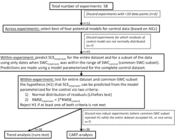
In order to test whether the moisture response of SCE as observed in the control plots can be used to predict SCE un-der altered rainfall patterns, we followed the protocol pre-sented in Fig. 2. We first tested which of four models best fit-ted SCEcontrol. These models take into account SWC as well
as ST, because the latter is an important driver of fluctuation in SCE over time. Soil temperatures hardly differed between control and treatment plots (data not shown). For this and fur-ther analyses, experiments with no more than 10 data points were discarded. The four models (which have been used pre-viously, see, for example, Curiel Yuste et al., 2003; Kopittke et al., 2013) were
log(SR)=a+bST+cSWC, (1)
log(SR)=a+bST+log(c+dSWC), (2)
log(SR)=a+bST+log(c+dSWC+eSWC2), (3)
log(SR)=a+bST+cSWC+dSWC2. (4)
These four models all reflect an exponential relationship be-tween SCE and ST; the relationship bebe-tween log(SCE) and SWC is linear, quadratic, exponential linear and exponential quadratic for models 1, 2, 3 and 4, respectively. The first two models characterize soil moisture response as a monotonic function (increasing whend is positive), whereas models 3
and 4 allow non-monotonic responses. Model coefficients and goodness-of-fit parameters for all sites and models are presented in Supplement Tables S3 and S4.
Model selection was based on the second-order Akaike in-formation criterion (AICc). Across all sites, model 4 showed a significantly lower AICc than all other models (Wilcoxon sign rank test,p <0.05). Therefore, we opted to use model 4
for all subsequent analyses. However, residuals were not nor-mally distributed for seven experiments, which were there-fore discarded from the subsequent analyses (note that for these experiments the normal distribution criterion was usu-ally not met for any of the other three models either). Ar-guably, we could have opted for the best of the four models for a given experiment instead of the best model across ex-periments. We opted for the latter to avoid possible artifacts related to using different models for different sites. More-over, results were similar when using models 1–3 (but fewer sites were eligible for the tests, data not shown),
We parameterized model 4 for each of the 45 remain-ing experiments usremain-ing the control data, and used the result-ing model coefficients specific to each site to test whether SCEtreatment could be predicted. Subsequently, these results
were used to test our hypothesis that the moisture response of SCE as observed in the control plots can be extrapolated to predict SCEtreatment. We set forward two criteria
Figure 1. (a)Overview of the magnitude and direction of precipitation effect on soil CO2efflux (SCE) for the different experiments. Arrows point from control precipitation to treatment precipitation (averaged over different years in case of multi-year data). Crosses localize control conditions in terms of annual precipitation and mean annual temperature (MAT). Black arrows indicate a positive correlation between precip-itation manipulation and SCE, i.e., an increase of SCE when precipprecip-itation increases, or a decrease of SCE when precipprecip-itation is reduced. Gray arrows indicate negative correlations (which could be considered to reflect somewhat unexpected results). Bold arrows represent significant differences between SCE treatment and SCE control (p <0.05), while thin arrows reflect non-significant differences (repeated measures ANOVA). Panel(b)shows the biomes that are represented by our data set (biome figure adapted from Chapin et al., 2002).
1. The difference between SCEtreatment predicted by the
control model (further termed “predicted SCEtreatment”)
and observed SCEtreatment followed a normal
distribu-tion (Lilliefors test).
2. The root-mean-square error (RMSE) for predicted SCEtreatment was less than double the RMSE for
pre-dicted SCEcontrol. This second criterion is critical,
be-cause it indicates the goodness of fit to SCEtreatment,
tak-ing into account the performance of the control model. Because no generally accepted threshold for accurate data–model agreement exists, we opted for a stringent threshold where RMSEtreatment<2RMSEcontrol, which
in our case was exceeded in only a few sites (Appendix Table C1). Visual inspection of the figures for pre-dicted versus measured values (Fig. S3) and the resid-uals (Fig. S1) indicated that this criterion was justified for rejecting H1.
When both conditions were fulfilled, the prediction of SCEtreatment was considered reasonable and H1 was not
re-jected. It was rejected when at least one of both criteria was not met.
Rejection of H1 may have resulted from structural changes in the ecosystem, or may merely reflect erroneous extrap-olation beyond the range of the conditions observed in the control. To test whether such erroneous extrapolation was re-sponsible for rejection of H1, we performed the two tests for H1 also on a subset of the data, using only dates when SWCtreatment was within the range of SWCcontrol (further
simply referred to as “common SWC subset”). We consider the results robust when the outcomes of the analysis for the entire data set and for the common SWC subset agree and po-tential rejection of H1 is unlikely due to extrapolation. Only for such robust sites were subsequent analyses performed.
Figure 2.Protocol of the analyses performed to test the hypothesis (H1) that the moisture response of soil CO2efflux as observed in the control plots (SCEcontrol)can be used to predict soil CO2efflux in
the precipitation manipulation treatment (SCEtreatment). The
num-ber of sites for each step and the reasons for discarding experiments from further analyses are displayed.
(MAP), mean annual temperature (MAT), an aridity index (MAP/2MAT), treatment manipulation type (drought or ir-rigation experiment or altered precipitation pattern with-out a change in total precipitation) and manipulation tech-nique (roofs, shelters, retractable curtains, troughs or irriga-tion), treatment manipulation duration (continuous manip-ulation, episodic manipulation or altered pattern during the entire experiment), number of years of experimental manip-ulation, and the percentage of measurement days for which SWCtreatment was either above or below the natural
bound-aries of SWCcontrol (i.e., an indication of potentially
erro-neous extrapolations beyond the range for which the model was parameterized). We further included as predictor vari-ables the total number of SCE measurements (N), the me-dian of the measurement interval (I, number of days), and N/I (which is low for sites with few and/or infrequent mea-surements; highest N/I is obtained for experiments with daily SCE measurements). As several experimental sites were rep-resented by more than one experiment, we weighted the CART analysis by the inverse of the number of experiments per site. For example, the Sevilleta experiment consisted of two different irrigation experiments, and therefore each ex-periment was weighted by 0.5 (Appendix Table C1).
To further analyze the possible cause for the failure of the control model to predict SCEtreatment, we examined the
course of a predictability index over time, which was calcu-lated for each measurement day as
Pi= |predicted SCEcontrol−observed SCEcontrol|
− |predicted SCEtreatment−observed SCEtreatment| (5)
where predicted SCEcontrol and predicted SCEtreatment are
both calculated using model 4 (see above) and parameterized using the control data. Hence, Pi indicates the predictabil-ity of SCEtreatment, but taking into account the predictions of
SCEcontrolat the same moment in time. Values of Pi around
zero indicate that the model parameterized for the control performs similarly for control and treatment, while nega-tive values indicate that the prediction of the treatment is worse than that of the control (and vice versa for positive values). For the current analysis, we are particularly inter-ested in the change of Pi over time. If Pi shows a trend to-wards increasingly negative values over time, then the pre-dictability of SCEtreatment becomes progressively worse. To
test whether there was a significant trend in Pi (e.g., a de-crease of Pi over time, or during part of the measurement pe-riod) we performed the runs test (non-parametric trend anal-ysis), dichotomized around the median (Davis, 2002). This test checks the randomness of sequences. It creates “runs”, defined as uninterrupted sequences of the same state (in this case either above or below the median), and then tests whether the number of runs is significantly different from what would be expected if they were randomly drawn from the same distribution. The runs test is thus not affected by the increased serial dependence of data with increasing mea-surement frequency, which is important because our study in-cludes experiments with different measurement frequencies.
2.2 Test for artifacts related to SWC measurements
The estimate of water availability obtained from the bucket model was then used to perform analyses analogous to those described above: coefficient estimates from a control model (in model 4, SWC was replaced by the water availability esti-mate from the bucket model, while ST did not change) were used to predict SCEtreatmentat each measurement date.
Sub-sequently, we tested H1 and estimated Pi, which was further analyzed for trends via the runs test. More details about this analysis based on the bucket model estimates of water avail-ability are given in the supporting information.
All analyses were performed using Matlab (2012b, The Mathworks Inc., Natick, MA). A comprehensive list of the abbreviations used in this study is provided in Table D1.
3 Results
3.1 General response of soil CO2efflux to precipitation
manipulation
Our data set covers different climate regions and biomes (Fig. 1 and Appendix Table A1), but the temperate zone is clearly dominant. Few experiments were conducted in the tropics (n=3), and we found no precipitation manipulation experiments with SCE measurements for the boreal zone. Forests, grasslands and shrublands are all well represented, but agricultural fields are not (only one site, with three ex-periments – Hohenheim; Appendix Table A1), and hydric sites are also represented by only one site (Clocaenog). Over-all, decreased precipitation reduced SCE, whereas enhanced precipitation increased SCE (Fig. 1), although for six exper-iments, we found a significant response of SCE in the oppo-site direction. Four of these were drought experiments (Clo-caenog, Solling, Tolfa and WalkerBranch_ Dry; Appendix Table B1), one was an irrigation experiment (Boston_ wet) and one was an experiment where only the precipitation pattern was altered, with little effect on total precipitation (RaMPsAlt; the manipulation slightly increased total rainfall, and decreased total SCE; Appendix Table B1).
3.2 Across-experiment variation in predictability of soil CO2efflux
We tested the goodness of the prediction of SCEtreatment on
the entire data set for each site, as well as on the common SWC subset (i.e., excluding dates for which SWCtreatment
was outside the range of SWCcontrol). For this, we started
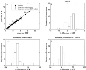
from the 45 experiments where the control model was of suf-ficient quality (see protocol in Fig. 2). For 38 of these 45 experiments subjected to this analysis, both tests gave the same outcome and results are considered robust (Appendix Table C1, column “Robust?”). These sites showed both over-and underestimations of SCEtreatment(Fig. 3a and Appendix
Table B1). Across all sites, using the common SWC subset instead of the entire data set had a minor effect on the differ-ence between predicted and observed SCEtreatment (Fig. 3c
Figure 3. (a)Predicted soil CO2efflux (SCE, µmol CO2m−2s−1) versus observed SCE for control, for the treatment when using the entire data set, and for the treatment when using the common SWC subset. Predictions of treatment SCE were based on the model parameterized for the control.(b–d)Histograms showing the fre-quency of occurrence for the percentage difference between ob-served and predicted for control, for the treatment when using the entire data set and for the treatment when using the common SWC subset. The percentage difference was calculated as 100·(average predicted – average observed)/average observed. For details, see Appendix Table C1.
and 3d), although for some sites, this reduction was substan-tial (see Appendix Table B1).
For the 38 experiments for which both the entire data set and the common SWC subset gave the same result (i.e., the experiments with robust results), H1 was rejected in only seven, while we could not reject the hypothesis for the re-maining 31 experiments (Appendix Table C1). The seven experiments for which H1 was rejected represent six inde-pendent sites (one site was represented by two experiments, Appendix Table C1). The 31 experiments for which H1 could not be rejected represented 14 different sites (Appendix Ta-ble C1).
To test whether artifacts related to SWC measurements were responsible for rejecting H1, we replaced SWC in model 4 with the bucket model results. This exercise pro-vided results of acceptable quality (i.e., normal distribution of the residuals and anR2≥0.30; see SI) for only 16 of the
Figure 4. Classification and regression tree (CART) showing for which groups of experiments our hypothesis (H1: the moisture re-sponse of soil CO2 efflux (SCE) as observed in the controls can be used to predict SCE in the treatment) could and could not be rejected. This CART analysis included as a weight factor the recip-rocal of the number of experiments per site to take into account their interdependence. The key predictor variable (the median measure-ment interval) is depicted at the top, and predictor variable thresh-olds are at the side of each branch. Below the terminal nodes, the values between brackets display: total number of experiments; num-ber of experiments for which H1 was not rejected - numnum-ber of ex-periments for which H1 was rejected. A list of all predictor variables included in the CART-analysis is given in the Methods section. This analysis used the 38 experiments for which results from the entire dataset and the common SWC subset agreed (i.e., robust results).
approach did not allow for this test. In any case, the bucket model approach indicates that artifacts related to SWC mea-surements are unlikely responsible for rejecting H1.
The CART analysis – which accounts for the dependence of results from different experiments within a single site (Ap-pendix Table C1) – indicated measurement frequency as the key predictor variable of whether or not H1 could be rejected. For experiments with median measurement intervals of SCE larger than 11 days, H1 was never rejected (Fig. 4), whereas H1 was rejected for 7 of the 14 experiments with intervals ≤11 days, which included all 5 experiments with daily mea-surements (Appendix Table C1). The CART analysis did not identify other predictive variables or thresholds.
3.3 Within-experiment variability in predictability of soil CO2efflux
A trend analysis of the predictability of SCEtreatment(Pi) was
made for the 38 experiments for which both the entire data set and the common SWC subset gave the same result (i.e., those indicated as robust in Appendix Table C1). When Pi varies around zero, predictions of SCEtreatment are
compa-rable to predictions of SCEcontrol. Negative values indicate
that the prediction of SCEtreatment was worse than that of
SCEcontrol(and vice versa for positive values – but these were
less abundant and always close to zero for all sites, Supple-ment Fig. S2). Significant trends in Pi reveal that model
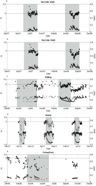
per-Figure 5.Time course of Pi (predictability index, large black and gray circles) for the five experiments for which our hypothesis was rejected and for which a significant trend was detected:(a) Sevil-leta_ Wet1,(b) Sevilleta_ Wet2, (c) Solling, (d) Stubai and (e) TurkeyPoint. Pi values close to zero indicate that SCEtreatmentwas
predicted similarly well compared to SCEcontrol, whereas values substantially below or above zero indicate the difference in pre-dictability of SCEtreatmentrelative to SCEcontrol. Negative values
indicate that the prediction of SCEtreatmentwas worse than that of
SCEcontrol, and vice versa for positive values. Large gray circles indicate when SWCtreatmentwas outside the range of SWCcontrol.
formance varied over time and thus suggest that the model parameterized for the control plots cannot reliably capture the variation in SCEtreatment. Whereas we detected a trend in
Pi for only 1 of the 31 experiments for which H1 was not rejected (SulawesiForest; see Supplement Fig. S3 for a vi-sual representation), we found a significant trend in the time course of Pi for five of the seven experiments for which H1 was rejected (Appendix Table C1). These five experiments were those with daily measurements of SCE. The time series of Pi for these five experiments is displayed in Fig. 5. For all other experiments, the course of Pi over time is shown in Supplement Fig. S2. Here we briefly describe the patterns observed for the five experiments for which H1 was rejected and revealed a trend in Pi (i.e., the five experiments with daily measurements of SCE). These patterns can expose the under-lying reasons for rejecting H1.
The Sevilleta experiment, which consisted of two differ-ent irrigation treatmdiffer-ents in a desert grassland, showed lit-tle effect on Pi in the first year, while a marked decrease in Pi occurred in the second year (Fig. 5a, b), particularly for the treatment plots receiving the more intense rainfall events (Sevilleta_Wet2). Here, Pi values remained below zero over two months, even though SWC was very similar in con-trol and treatment (Fig. 5b). Such erroneous predictions of SCEtreatment would, in the case of Sevilleta_Wet2, lead to
ca. 35 % underestimation of SCE over the entire measure-ment period (Appendix Table B1).
Likewise for Solling, despite SWCtreatment remaining
mostly within the range of SWCcontrol(Fig. 5c), Pi remained
below zero during part of the experiment. Of particular in-terest is the decline of Pi upon rewetting, which occurred in both treatment years and reflects an increase of SCEtreatment
(see Fig. S1). Recovery of Pi took about four months in the second treatment year, but insufficient data were available to really test for the duration of recovery. Nonetheless, estima-tions of SCEtreatment based on the control model would
un-derestimate SCEtreatmentby 33 % over the entire experimental
period (Appendix Table B1).
In contrast, in Stubai, the number of measurements was substantially reduced when selecting only the dates when SWCtreatment was within the range of SWCcontrol (n=103, which is exactly one-third of the total number of data, Fig. 5d). Nonetheless, H1 was rejected also when only the common SWC subset of measurements was used (Appendix Table C1). Pi remained below zero even when SWCtreatment
had recovered after the manipulation had ended. Moreover, Pi remained negative just before the initiation of the ma-nipulation in 2012 and across the three treatment years; this would result in an overestimation of SCE by 25 % when con-sidering only the common SWC subset (Appendix Table B1). At the TurkeyPoint site, Pi started declining before the onset of the manipulation (Fig. 5e). This caused dif-ficulty in distinguishing the effects of the manipulation from pre-treatment differences. Nonetheless, analysis of the residuals revealed that the difference between SCEcontrol
and SCEtreatment shifted after the manipulation had ended
(Fig. S1); whereas residuals for SCEtreatment were
consis-tently lower than residuals for SCEcontrol before and during
the manipulation, the opposite was true for all measurement dates after the manipulation period. This suggests that the manipulation induced substantial changes in the ecosystem. Over the entire data set, estimations of SCEtreatmentbased on
the control model would overestimate SCEtreatmentby 72 %
(Appendix Table B1).
4 Discussion
4.1 General response of soil CO2efflux to precipitation
manipulation
Precipitation manipulation experiments have been conducted mainly in the temperate zone, as shown in this study (with all but three experiments in temperate and subtropical regions) and in a general review by Beier et al. (2012). Particularly un-derrepresented in our study were the tropics and the boreal zone. Hence, it would be important to promote research in these regions for improving our global understanding of SCE responses to altered precipitation regimes. Also experiments in agricultural fields and on hydric soils are underrepresented in our data set, with only one site for each (Appendix Ta-ble A1). Forests, grasslands and shrublands in temperate and subtropical regions are all well represented in our data set.
In agreement with Wu et al. (2011), decreased precipita-tion typically reduced SCE, whereas enhanced precipitaprecipita-tion increased SCE (Fig. 1). However, some responses did not fit this pattern (Fig. 1). One reason why a reduction in rain-fall could stimulate SCE is related to the non-monotonic re-sponse of SCE to moisture. This is especially likely for the only hydric experiment in our data set, i.e., Clocaenog. This experiment showed a persistent increase in SCE following precipitation reduction (Sowerby et al., 2008), which is in line with the general observation of moisture responses of SCE in wetland ecosystems (Jungkunst and Fiedler, 2007). In addition, soil rewetting after a drought event can substan-tially increase SCE and lead to higher SCE at the annual scale in the treatment compared to the control (Borken et al., 1999). This was obviously the case in Solling (see below for more details).
4.2 Across-experiment variation in predictability of soil CO2efflux
The CART analysis indicated that sampling frequency was an overriding factor determining whether or not H1 was rejected. The higher the measurement frequency, the more likely H1 was rejected, and in all five experiments where SCE was measured daily, SCEtreatmentcould obviously not be
pre-dicted from SCEcontrol. Indeed, even when avoiding
frequency was thus crucial for detecting whether or not SCEtreatmentcould be predicted from the ST–SWC
relation-ship fitted to SCEcontrol. This result suggests that we may
have missed important SCEtreatmentresponses in experiments
with larger measurement intervals. Infrequent measurement schemes have insufficient capacity to detect shifts in the cli-mate dependencies of SCE, which implies that type 2 errors (i.e., failure to reject H1) for these experiments are probable, and this is an important call for the scientific community to revisit studies with discrete measurements. Our results em-phasize the need for high-frequency SCE measurements to fully capture the fast response of SCE to changes in precip-itation and other climatic variables such as temperature at multiple temporal scales (Vargas et al. 2012).
Nonetheless, of the 14 experiments with a measure-ment frequency<11 days (i.e., the threshold resulting from
the CART analysis), H1 could not be rejected for seven. These experiments represent in fact only four different sites (Duolun40, Duolun60, HarvardForest, Hohenheim_ LA, Ho-henheim_ LF, RaMPs_ Dry and RaMPs_ DryAlt; see Ap-pendix Table C1), and it is possible for these sites that the criteria set for rejecting H1 were too stringent. The difference in RMSE was particularly high for HarvardForest (1.72, Ap-pendix Table C1), and it is plausible that a more complete data set (i.e., more frequent measures) would have given a different outcome (see also Supplement Fig. S2). On the other hand, experimental duration was rather short for (i) the two experiments of the Mongolian Duolun grassland site, for which SCE was measured weekly, but only for about six months (Supplement Fig. S2), and (ii) for the experi-ments in Hohenheim, where SCE was measured for ca. 10 months, precluding firm conclusions. Alternatively, not re-jecting H1 for some experiments that provided frequent mea-sures of SCE may reflect real variability in the potential for predicting SCEtreatmentfrom relations found for the control.
The RaMPs experiment illustrates that in some cases, pre-dicting SCEtreatmentfrom SCEcontrolcould be possible. This
experiment covered four manipulation years, during which SCE was measured at ca. 5-day intervals during the growing season (Appendix Table C1). The fact that H1 could not be rejected and no trend was observed for the two experiments of this site is consistent with the study by Fay et al. (2011). They reported that interannual rainfall variability was more of a determinant for most ecosystem processes studied at the RaMPs site than the manipulations applied. Hence, the ex-perimental manipulation seems not to have pushed the sys-tem beyond a threshold that would have yielded different responses of SCEtreatment. Whether this is related to the
silience of the ecosystem, or to the manipulation applied, re-mains to be tested and is an important discussion pertinent for other and future experiments.
4.3 Within-experiment variability in predictability of soil CO2efflux
We examined in more detail the predictability index of SCEtreatmentfor experiments with daily SCE measurements.
This detailed analysis allows for detecting patterns and un-raveling mechanisms that may remain unseen when study-ing only seasonal or annual totals. In our study, this analysis revealed various patterns for the five experiments providing daily SCE measurements, i.e., the experiments with the most reliable data sets. These are discussed in the following para-graphs to illustrate that various mechanisms can make the current moisture responses of SCE inappropriate for extrap-olation to a future precipitation pattern, and to indicate which measurements are important to be obtained in future experi-ments if we are to understand the response of SCE to altered precipitation.
In the Sevilleta experiment, SCEtreatmentwas equally well
predicted as SCEcontrol(no marked change in Pi) in the first
year. In the second year and particularly for treatment plots receiving the most intense irrigation (Sevilleta_Wet2), Pi de-creased strongly. The results from this site indicate that rain-fall intensity is an important factor determining variation in SCE. Vargas et al. (2012) attributed the observed increase in SCE in irrigated plots to an enhancement of the autotrophic component of SCE. This example thus illustrates that if we are to understand the mechanisms driving moisture responses of SCE, measurements of the autotrophic and heterotrophic components of SCE are required. These data are not currently available for any the experiments presented in this review.
For the Sevilleta experiment, Thomey et al. (2011) fur-ther indicated the importance of moisture in deep soil lay-ers, which was replenished only when applying the most in-tense precipitation manipulation (one 20 mm rain event per month, Sevilleta_Wet2 in the current study), but not as much by more frequent but less intense rain events (four 5 mm rain events per month, Sevilleta_Wet1 in the current study). This finding emphasizes the need for precipitation experiments to measure SWC over the entire rooting zone, and not only top-soil SWC (as is typically the case; see Vicca et al., 2012a, for a discussion on this topic). Mechanistic understanding of such effects could be further improved by also measur-ing predawn leaf water potential, which indicates the stress level as experienced by the plants (Vicca et al., 2012a).
For the Solling experiment, Pi decreased markedly upon rewetting. The Pi decrease was due to suddenly higher ob-served SCEtreatmentthan predicted (see residuals in Fig. S1),
through reduced aggregate stability (Borken and Matzner, 2009; Denef et al., 2001). In the case of Solling, the in-crease of SCE after rewetting more than compensated for re-ductions in SCE during the dry period (Appendix Table B1; see Borken et al., 1999, for details about SCE in the Solling experiment). Although such overcompensation for drought-related decreases of SCE after rewetting is not a universal phenomenon (Borken and Matzner, 2009), Birch effects are commonly observed in various ecosystems (Kim et al., 2012; Inglima et al., 2009; Jarvis et al., 2007), but are not usually accounted for by models. To improve our understanding of the Birch effect, and because it is supposed to be a primarily microbially mediated phenomenon, we again stress that it is necessary to separate heterotrophic from autotrophic respira-tion in future SCE monitoring experiments.
At the Stubai grassland site, Pi decreased sharply over the course of several drought manipulations performed in consecutive years. Pi broadly followed the course of SWCtreatment, but was mostly outside the range of SWCcontrol.
In contrast to Solling, Pi returned rapidly to high values after rewetting, despite a noticeable Birch effect (Fig. S1), and ap-peared to be mostly determined by SWC. Nonetheless, when excluding the dates when SWCcontrolwas outside the range of
SWCtreatment, H1 was still rejected (Appendix Table C1) and
Pi remained below zero after the precipitation manipulation, (especially after the 2012 manipulation, Fig. 5), resulting in a substantial overestimation (25 %) of SCEtreatmentwhen
us-ing the common SWC subset (Appendix Table B1). This indicates that SCE did not fully recover after the drought, which could be related to structural changes in soil chemical properties, soil physical properties, microbial communities and/or vegetation. This list of potential underlying reasons for the observed patterns makes clear that a holistic approach – considering also various other ecosystem properties and processes – is required if we are to mechanistically under-stand how SCE responds to altered precipitation.
For the TurkeyPoint experiment, Pi was low during and after the manipulation period. This pattern corresponds to aboveground observations made at the site where the rain-fall exclusion was conducted during spring, when tree growth is greatest in this region (Hanson and Weltzin, 2000). Tree growth was strongly influenced by the precipitation exclu-sion and did not fully recover after the drought period. More-over, tree growth terminated earlier in the drought plots as compared to the control plots (MacKay et al., 2012). Strikingly, treatment-induced changes to tree growth dynam-ics positively influenced SCE, as residuals in autumn were higher for the treatment than for the control (Fig. S1). Possi-ble mechanisms to explain this lag effect could be the Birch effect as described above, or the decomposition of roots that died during drought-induced senescence. Moreover, plants can allocate large but variable fractions of their photosyn-thates belowground (Vicca et al., 2012b), with potentially rapid and strong effects on the autotrophic component of SCE (Bahn et al., 2008; Högberg et al., 2001; Kuzyakov and
Gavrichkova, 2010). Hence, the results from this experiment also emphasize the need to separate autotrophic from het-erotrophic respiration to fully explore the exact mechanisms underlying SCE responses.
The above list of potential mechanisms that can alter the moisture response of SCE when the precipitation regime changes is of course incomplete. Several other mechanisms can play at different levels (from community level to soil and microbial level). It is beyond the scope of this study to go into detail about all potential mechanisms. For reviews about various changes in the ecosystem under altered precipitation regimes, we refer the reader to Borken and Matzner (2009), Schimel et al., (2007) and van der Molen et al. (2011). Here, we want to emphasize the need for a holistic approach in experiments that aim to elucidate how SCE is affected by changes in precipitation regime.
4.4 A novel approach revealing limitations of current
experiments and recommendations for future experiments
At present, inter-site comparison of effects of altered pre-cipitation is seriously hampered by the lack of data neces-sary to quantify the treatment as experienced by the biota (i.e., the actual treatment; Vicca et al., 2012a). Without such data, conventional meta-analysis of cross-experiment varia-tion in ecosystem responses to precipitavaria-tion manipulavaria-tion is prone to artifacts related to the enormous variation in the ac-tual treatment; the magnitude, timing and duration of drought and rain events vary substantially among experiments, and soil type and rooting depth considerably influence the way plants and microbes experience a treatment (Vicca et al., 2012a). The novel approach presented here was developed specifically to avoid these problems. This is accomplished by analyzing within-experiment responses (through calculation of a predictability index) prior to across-experiment com-parison (via CART analysis). Although treatments also re-main largely incomparable with this method (hence, if cross-experiment differences were to occur, these could be due either to variation in the actual treatment or to differences in ecosystem response, or a combination), our method does provide mechanistic insight into the responses to altered pre-cipitation. Importantly, the results are less prone to the large variation in the actual treatment. It would be particularly in-teresting to combine this approach with a quantification of the actual treatment such that moisture responses of SCE in various ecosystems can be elucidated.
Fig. 2). For this reason, and because the CART analysis sug-gests that frequent SCE measurements are essential to detect deviations of the moisture response of SCE in the treatment as compared to the control, we recommend that future exper-iments that aim to test the response of SCE to altered pre-cipitation seek to obtain high-frequency SCE measurements. This recommendation also applies to variables such as pho-tosynthesis and ecosystem respiration that can be measured at high frequency with automated cuvettes and are therefore suitable for testing as in this study.
5 Concluding remarks
Is it possible to extrapolate the relationships between SCE and its abiotic drivers – soil temperature and soil moisture – to predict SCE responses to changes in precipitation pat-terns? According to our results, the most justified answer to this question is “no”; although for the majority of the experiments we could not falsify the hypothesis that we can predict SCE under altered precipitation regimes from current-climate observations. As discussed, all experiments with daily SCE measurements (i.e., the experiments with the data sets most reliable for this exercise) revealed that SCE in the altered precipitation treatment could not be predicted from the control observations. We postulate that at least some of the experiments with infrequent measurement schemes provided insufficient capacity to detect shifts in the climate dependencies of SCE. In other words, crucial patterns in SCE likely went undetected for these experiments. Importantly, the erroneous predictions in the experiments with daily SCE measurements were not related to extrapolation beyond the range for which the model was parameterized. Instead, these experiments provide insights of likely mechanisms (e.g., the Birch effect) that cause SCE in the treatment to deviate from what would be expected from the control observations.
Using single-factor experiments, our study demonstrated that current relationships between SCE and soil moisture should not be extrapolated to predict SCE when precipita-tion patterns change. However, climate change involves not only changes in precipitation regimes but also other environ-mental forcing factors. Droughts are often associated with warm periods or heat waves, and in combination with a heat wave, drought effects are typically exacerbated (Reich-stein et al., 2013). This implies that thresholds for structural changes in the ecosystem may be passed earlier, which most likely makes predictions based on current-climate observa-tions even less reliable than our analysis may suggest.
At present, the available data do not enable full elucidation of the mechanisms that complicate extrapolation of current-climate observations of the moisture response of SCE to pre-dict SCE when rainfall patterns alter, and this likely applies also to other ecosystem and carbon cycle processes. If we are to fully understand ecosystem responses to altered precipita-tion, we need more experiments establishing response
func-tions across a broader range of precipitation regimes, annual temperatures, soil moisture conditions and vegetation types (especially in boreal and tropical regions). Such experiments should make accurate measurements of water availability, they should consider both instantaneous responses and the potential legacy effects of climate extremes, and would ben-efit from a holistic approach that allows for elucidation of underlying mechanisms. Future studies should make partic-ular effort to obtain high-frequency measurements, which – as we demonstrated – are essential for capturing dynamic re-sponses during drying and after rewetting, and for quantify-ing their implications for the carbon cycle in a more extreme climate.
Author contributions
S. Vicca conceived the manuscript, and performed the analy-ses and writing. M. Bahn, M. Estiarte and I. A. Janssens sub-stantially contributed to the discussions prior to the writing. E. E. van Loon focussed specifically on the statistical analy-ses. All co-authors contributed with data and/or intellectual input during the writing process.
The Supplement related to this article is available online at doi:10.5194bg-11-2991-2014-supplement.
Global Climate Change Small Watershed Project grant to John Zak and a National Park Service grant to John Zak and David Tissue. L. P. Bentley was funded by the United States Environmental Protection Agency (EPA) under the Greater Research Opportunities (GRO) graduate program. E. Lellei-Kovacs acknowledges support provided through the research grant of the EU FW5 VULCAN project and the NKFP-3B/0008/2002 grant from the Hungarian Government. The research of M. Estiarte and J. Peñuelas was supported by the Spanish government grants CGL2010-17172 and Consolider Ingenio MONTES (CSD2008-00040), and by the Catalan government grant SGR2009-458. The Brandbjerg experiment (Climaite) was funded by the Villum Foundation. I thank Lola and Mauro for making my life more colorful. Lastly, we wish to thank the editor and three anonymous reviewers for their positive assessment of our work and the insightful suggestions that improved this paper.
Appendix A
Table A1.Information about the precipitation manipulation experiments: latitude (Lat), longitude (Long), mean annual precipitation (MAP, mm), mean annual temperature (MAT,◦C), Köppen classification (Köppen class.), vegetation type hydrology (Hydr.), manipulation type
(Manip. type: drying experiment (–), irrigation experiment (+)or experiment in which the pattern of precipitation was altered, but not the total amount of precipitation (0)), duration of the manipulation (episodic manipulation over a few weeks while the rest of the year is unaltered (Epis) versus continuous drying/irrigation during entire growing season or year (Cont) versus altered rainfall pattern during entire year (ContAlt)), the percentage of clay in the soil, the depth of SWC measurements (cm), and a key reference for each experiment (if available). Species composition for all sites is given in Supplement Table S1. We distinguish between sites used only for Fig. 1 (not used for further analysis because there were not enough data points to generate reliable model fits (n≤10)), sites discarded from further analyses because of non-robust results (see Appendix Table C1), and sites used for all analyses.
Experiment Lat Long MAP MAT Köppen class. Vegetation Hydr. Manip. type Duration manip. % clay SWC depth Key reference
Sites included in Fig. 1, but excluded from other analyses because of too few data or non-normal distribution of model residuals for SCEcontrol
Almería 37.09 −2.08 274 17 BSk shrubland xeric – Cont 7 0–5 Maestre et al. (2013) Achenkirch 47.58 11.64 1480 5.7 Cfb forest mesic – Epis 28 5 Schindlbacher et al. (2012) BigBend_S 29.30 −103.17 370 24.2 BWh shrubland xeric + Epis 8 15 Patrick et al. (2007) BigBend_W 29.30 −103.17 370 24.2 BWh shrubland xeric + Epis 8 15
BigBend_SW 29.30 −103.17 370 24.2 BWh shrubland xeric + Epis 8 15
Garraf 41.30 1.82 552 15.6 Csa shrubland xeric + Epis 18 0–15 Beier et al. (2004) Prades 41.35 1.03 663 11.7 Csa forest xeric – Epis 21 0–25 Ogaya et al. (2011) RaMPs_Alt 39.10 −96.60 835 13 Cfa grassland mesic 0 ContAlt 32 0–15 Fay et al. (2011) ThuringerSchiefer5 50.48 11.60 1000 6.5 Cfb grassland mesic – Epis 25 0–10 Kahmen et al. (2005) ThuringerSchiefer6 50.48 11.58 1000 6.5 Cfb grassland mesic – Epis 25 0–10
ThuringerSchiefer19 50.48 11.26 1000 6.5 Cfb grassland mesic – Epis 22 0–10
Tolfa_Dry 42.15 11.93 729 13 Csa forest xeric – Cont 6 0–10 Cotrufo et al. (2011)
Tolfa_Wet 42.15 11.93 729 13 Csa forest xeric + Epis 6 0–10
Sites included in Fig. 1 and hypothesis tests, but excluded from CART analysis because of non-robust results (see Appendix Table C1)
Boston_dry 42.39 −71.22 1063 10.3 Dfa grassland mesic – Cont 9 0–30 Suseela et al. (2012) Caxiuana −1.73 −51.46 2314 26.9 Af forest mesic – Cont 10 0–30 Sotta et al. (2007) Hohenheim_LALF 48.70 9.18 679 8.7 Cfb agriculture mesic – Epis 22 0–15
Oldebroek 52.40 5.90 1042 10.1 Cfb shrubland mesic – Epis 8 0–50 Kopittke et al. (2013) SulawesiCacao −1.55 120.02 2092 25.5 Af forest mesic – Cont 14 5 van Straaten et al. (2010) ThuringerSchiefer2 50.41 11.63 1000 6.5 Cfb grassland mesic – Epis 24 0–10 Kahmen et al. (2005) ThuringerSchiefer3 50.41 11.63 1000 6.5 Cfb grassland mesic – Epis 23 0–10
Sites included in all analyses
Aranjuez 40.03 −3.54 349 15 Csa grassland xeric – Cont 6 0–5 Escolar et al. (2012) Boston_wet 42.39 −71.22 1063 10.3 Dfa grassland mesic + Cont 9 0–30 Suseela et al. (2012) Brandbjerg 55.88 11.97 613 8 Cfb shrubland mesic – Epis 2 20 Selsted et al. (2012) Clocaenog 53.05 −3.47 1550 8.2 Cfb shrubland hydric – Epis 50 7 Sowerby et al. (2008) Coulissenhieb 50.14 11.87 1160 5.3 Cfb forest mesic – Epis 19 10 Muhr and Borken (2009) Duolun_20 42.02 116.17 385 2.1 Dwb grassland mesic – Cont 17 0–10
Duolun_40 42.02 116.17 385 2.1 Dwb grassland mesic – Cont 17 0–10 Duolun_60 42.02 116.17 385 2.1 Dwb grassland mesic – Cont 17 0–10
HarvardForest 42.54 −72.17 1100 6 Dfb forest mesic + Epis 18 5 Borken et al. (2006) Hohenheim_LA 48.70 9.18 679 8.7 Cfb agriculture mesic – Epis 22 0–15 Poll et al. (2013) Hohenheim_LF 48.70 9.18 679 8.7 Cfb agriculture mesic 0 ContAlt 22 0–15
Kiskunsag 46.88 19.38 505 10.4 Cfb shrubland xeric – Epis 2 0–20 Lellei-Kovacs et al. (2011) Mols 56.38 10.95 550 7.7 Cfb shrubland mesic – Epis 6 0–40 Beier et al. (2004) PortoConte 40.62 8.17 640 16.8 Csa shrubland xeric – Epis 13 0–10 de Dato et al. (2010) RaMPs_Dry 39.10 −96.60 835 13 Cfa grassland mesic – Cont 32 0–15
RaMPs_DryAlt 39.10 −96.60 835 13 Cfa grassland mesic – ContAlt 32 0–15
Sevilleta_Wet1 34.34 −106.73 250 13.2 BSk grassland xeric + ContAlt 10 0–15 Thomey et al. (2011) Sevilleta_Wet2 34.34 −106.73 250 13.2 BSk grassland xeric + ContAlt 10 0–15
Solling 51.52 9.56 1090 6.4 Cfb forest mesic – Epis 32 10 Borken et al. (1999)
Stubai 47.13 11.31 915 6.3 Dfc grassland mesic – Epis 16 5
SulawesiForest −1.49 120.05 2901 20.6 Af forest mesic – Cont 39 5 van Straaten et al. (2011) ThuringerSchiefer1 50.41 11.63 1000 6.5 Cfb grassland mesic – Epis 24 0–10 Kahmen et al. (2005) ThuringerSchiefer4 50.46 11.59 1000 6.5 Cfb grassland mesic – Epis 25 0–10
ThuringerSchiefer7 50.48 11.56 1000 6.5 Cfb grassland mesic – Epis 25 0–10 ThuringerSchiefer8 50.47 11.50 1000 6.5 Cfb grassland mesic – Epis 22 0–10 ThuringerSchiefer9 50.43 11.51 1000 6.5 Cfb grassland mesic – Epis 23 0–10 ThuringerSchiefer10 50.40 11.45 1000 6.5 Cfb grassland mesic – Epis 27 0–10 ThuringerSchiefer11 50.38 11.45 1000 6.5 Cfb grassland mesic – Epis 23 0–10 ThuringerSchiefer12 50.41 11.38 1000 6.5 Cfb grassland mesic – Epis 32 0–10 ThuringerSchiefer13 50.42 11.39 1000 6.5 Cfb grassland mesic – Epis 31 0–10 ThuringerSchiefer14 50.45 11.41 1000 6.5 Cfb grassland mesic – Epis 27 0–10 ThuringerSchiefer15 50.45 11.41 1000 6.5 Cfb grassland mesic – Epis 25 0–10 ThuringerSchiefer16 50.44 11.36 1000 6.5 Cfb grassland mesic – Epis 25 0–10 ThuringerSchiefer17 50.44 11.34 1000 6.5 Cfb grassland mesic – Epis 28 0–10 ThuringerSchiefer18 50.46 11.35 1000 6.5 Cfb grassland mesic – Epis 24 0–10
Appendix B
Table B1.For each experiment, the percentage change in precipitation is given, along with the average of observed and predicted soil CO2efflux (SCE; µmol CO2m−2s−1)for control and treatment in all experiments. “Sign. level” indicates whether the difference between treatment and control SCE measurements was significant atp <0.01 (**), atp <0.05 (*) or not significant (ns) according to repeated measures ANOVA. For the treatment, averages are also shown for the subset including only days where SWCtreatmentis within the range of
SWC observed in the control (common SWC subset). Averages were computed over the entire measurement period. Predictions are based on the model parameterized by the control data (model 4; see Methods and Supplement Table S3 for details). The percentage difference between predicted and observed is calculated as 100·(average predicted – average observed)/average observed. Positive values indicate overestimates, whereas negative values indicate that predicted SCE underestimated observed SCE. The percentage change in precipitation was calculated from precipitation data, averaged for the entire duration of the experiment. Negative values indicate a reduction of precipitation, while positive numbers indicate an increase in precipitation.
OBSERVED PREDICTED % difference
Experiment % change control treatment Sign. level control treatment treatment control treatment treatment
in precip. common SWC subset common SWC subset
Appendix C
For each experiment, we either fitted model 4 to the data of the control plots using the entire data set or to a subset of the data, including only the days where SWCtreatment is
within the range of SWC observed in the control (i.e., com-mon SWC subset). Subsequently, we tested the hypothesis that the moisture response of soil CO2efflux (SCE) as
Table C1.For each experiment, we present theR2of the model fitted to the data of the control plots, the number of data points (N) and the median interval (in days) between two consecutive measurements of soil CO2efflux (I). We also show the results of the two tests that we performed to test our hypothesis. For both the entire data set and the common SWC subset, “h1” is thepvalue of the Lilliefors test for normality, “h2” shows the ratio of RMSEtreatmentto RMSEcontroland “H” indicates whether or not H1 was rejected (see Fig. 2 and Methods
for details). Experiments for which both the entire data set and the common SWC subset gave the same result are indicated with “yes” in the column “Robust?”. The weight (W) used in this CART analysis is given (Wis calculated as 1/number of experiments per site that are used in CART). The results of the trend analysis on the time course of the predictability index of SCEtreatment(Pi, runs test dichotomized around the
median) are presented in the column “Trend”, with 0 indicating that no trend was detected and 1 indicating a significant trend for Pi versus time. When the rainfall manipulation was initiated more than one year before the start of SCE measurements, trend analysis is considered irrelevant. This is indicated as NA, followed by the result of the trend analysis in parentheses. Note that this table includes only results for experiments with > 10 data points and for which residuals of the control were normally distributed. Values in bold highlight the reason for rejecting H1.
Entire data set Common SWC subset
Experiment R2 N I h1 h2 H h1 h2 H Robust? W Trend
Aranjuez 0.37 29 35 0.50 1.06 0 0.50 1.06 0 Yes 1 0
Boston_dry 0.93 11 31 0.50 4.29 1 0.50 1.12 0 No NA NA(0)
Boston_wet 0.93 11 31 0.50 1.74 0 0.50 1.22 0 Yes 1 NA(0)
Brandbjerg 0.60 173 16 0.08 1.30 0 0.50 1.10 0 Yes 1 0
Caxiuana 0.49 22 15 0.15 2.35 1 0.50 1.55 0 No NA 0
Clocaenog 0.59 90 15 0.50 1.09 0 0.50 1.09 0 Yes 1 NA(0)
Coulissenhieb 0.86 35 9 0.09 2.41 1 0.13 2.43 1 Yes 1 0
Duolun_20 0.53 23 8 0.04 1.06 1 0.01 1.05 1 Yes 0.33 0
Duolun_40 0.53 23 8 0.07 1.09 0 0.08 1.09 0 Yes 0.33 0
Duolun_60 0.53 23 8 0.17 1.29 0 0.32 1.26 0 Yes 0.33 0
HarvardForest 0.82 43 7 0.50 1.72 0 0.50 1.72 0 Yes 1 0
Hohenheim_LA 0.71 38 7 0.50 1.20 0 0.50 1.21 0 Yes 0.5 0
Hohenheim_LALF 0.71 38 7 0.06 1.14 0 0.02 1.13 1 No NA 0
Hohenheim_LF 0.71 38 7 0.50 0.91 0 0.50 0.92 0 Yes 0.5 0
Kiskunsag 0.34 66 27 0.50 0.99 0 0.50 1.04 0 Yes 1 NA(0)
Mols 0.80 18 24 0.18 1.67 0 0.50 1.44 0 Yes 1 NA(0)
Oldebroek 0.73 73 15 0.03 1.36 1 0.50 1.07 0 No NA 1
PortoConte 0.30 47 36 0.50 0.97 0 0.37 0.98 0 Yes 1 0
RaMPs_Dry 0.47 74 5 0.50 0.94 0 0.50 0.92 0 Yes 0.5 0
RaMPs_DryAlt 0.45 73 5 0.50 1.29 0 0.50 1.26 0 Yes 0.5 0
Sevilleta_Wet1 0.38 163 1 0.00 1.47 1 0.01 1.39 1 Yes 0.5 1
Sevilleta_Wet2 0.38 163 1 0.50 2.53 1 0.42 2.53 1 Yes 0.5 1
Solling 0.85 264 1 0.00 2.60 1 0.00 2.59 1 Yes 1 1
Stubai 0.66 309 1 0.00 4.92 1 0.06 2.08 1 Yes 1 1
SulawesiCacao 0.37 46 14 0.00 13.14 1 0.50 1.29 0 No NA 1
SulawesiForest 0.39 59 14 0.50 1.73 0 0.33 0.89 0 Yes 1 1
ThuringerSchiefer1 0.72 14 22 0.11 1.28 0 0.30 1.45 0 Yes 0.07 0
ThuringerSchiefer2 0.81 13 24 0.17 1.95 0 0.03 2.38 1 No NA 0
ThuringerSchiefer3 0.35 13 24 0.04 0.87 1 0.11 0.72 0 No NA 0
ThuringerSchiefer4 0.59 14 22 0.50 0.85 0 0.50 0.88 0 Yes 0.07 0
ThuringerSchiefer7 0.72 14 22 0.50 1.53 0 0.50 1.47 0 Yes 0.07 0
ThuringerSchiefer8 0.75 15 24 0.33 1.57 0 0.50 1.62 0 Yes 0.07 0
ThuringerSchiefer9 0.83 15 24 0.32 1.26 0 0.32 1.26 0 Yes 0.07 0
ThuringerSchiefer10 0.76 14 22 0.34 1.12 0 0.34 1.12 0 Yes 0.07 0
ThuringerSchiefer11 0.67 13 27 0.13 1.14 0 0.13 1.14 0 Yes 0.07 0
ThuringerSchiefer12 0.52 14 23 0.50 0.88 0 0.50 0.94 0 Yes 0.07 0
ThuringerSchiefer13 0.73 14 23 0.13 1.18 0 0.20 1.37 0 Yes 0.07 0
ThuringerSchiefer14 0.86 12 26 0.22 1.13 0 0.08 1.18 0 Yes 0.07 0
ThuringerSchiefer15 0.96 14 26 0.50 1.44 0 0.50 1.47 0 Yes 0.07 0
ThuringerSchiefer16 0.73 15 24 0.14 0.95 0 0.27 0.95 0 Yes 0.07 0
ThuringerSchiefer17 0.83 14 22 0.13 1.86 0 0.38 1.62 0 Yes 0.07 0
ThuringerSchiefer18 0.83 14 22 0.50 1.18 0 0.50 1.18 0 Yes 0.07 0
TurkeyPoint 0.85 106 1 0.04 3.59 1 0.04 3.63 1 Yes 1 1
WalkerBranch_Dry 0.59 20 38 0.50 1.46 0 0.50 1.42 0 Yes 0.5 0
Appendix D
Table D1.List of abbreviations.
CART classification and regression tree
H1 hypothesis that the relationship between SCE and ST and SWC observed from fluctuations over time in the control plots can be extrapolated to predict SCE in plots exposed to a different precipitation regime
MAP mean annual precipitation
MAT mean annual temperature
Pi predictability index, calculated as the absolute error of predicted soil CO2efflux in the treatment reduced by the absolute error of predicted soil CO2efflux in the control at a specific moment (see Eq. 5). Pi values close to zero indicate that SCEtreatmentwas predicted similarly well compared to SCEcontrol, whereas
values substantially below or above zero indicate the difference in predictability of SCEtreatmentrelative to SCEcontrol. Negative values indicate that the prediction
of SCEtreatment was worse than that of SCEcontrol, and vice versa for positive
values.
SCE soil CO2efflux
SCEcontrol soil CO2efflux in the control SCEtreatment soil CO2efflux in the treatment
SWC volumetric soil water content
SWCcontrol volumetric soil water content in the control SWCtreatment volumetric soil water content in the treatment
common SWC subset data set using only dates when SWCtreatmentwas within the range of SWCcontrol