REALISM
AND
QUANTUM
SURREALISM
Master’s thesis
Presented to the Graduate Program in Physics of the
Universidade Federal de Minas Gerais
Author: Mateus Araújo Santos
Supervisor: Marcelo O. Terra Cunha
the world view that quantum mechanics represents. At least I do, because I’m an old enough man that I haven’t got to the point that this stuff is obvious to me. Okay, I still get nervous with it. And therefore, some of the younger students. . . you know how it always is, every new idea, it takes a generation or two until it becomes obvious that there’s no real problem. It has not yet become obvious to me that there’s no real problem. I cannot define the real problem, therefore I suspect there’s no real problem, but I’m not sure there’s no real problem.
À minha Luciana, por ter me feito um homem feliz e por ter conseguido controlar seus ciúmes dessa minha amante.
Aos meus pais, por serem quem são, e por me tornarem quem sou. Seu apoio foi e ainda é indispensável.
Ao meu orientador Marcelo Terra Cunha, por ter me dado a liberdade de putanejar enquanto eu podia, e por ter me mandado trabalhar quando eu precisava.
Ao meu grande amigo Marco Túlio Quintino, sem quem essa dissertação seria muito pior.
Ao Marcelo França, pelas conversas fiadas que me impediam de trabalhar, e por me impedir de ignorar suas sugestões.
A Gláucia Murta, pela ajuda indispensável em ler e reler a dissertação em busca de erros e passagens obscuras. Qualquer falha de matemática ou de estilo que tenha permanecido no texto é culpa dela. Também agradeço por ser um recurso local capaz de realizar protocolos inacessíveis a uma pessoa altamente não-local.
Aos meus amigos da Pós, agradeço pelo bom ambiente. Vocês tornam possível ser feliz e aprender física.
Aos professores da Pós, por tudo o que me ensinaram, e por tudo o que não me ensinaram.
Contents 4
Introduction 8
Notation and definitions 10
1 Ontological embeddings of quantum theory 11
1.1 What is an ontological theory? . . . 11
1.1.1 On mixed states and POVMs . . . 12
1.2 Ontological models . . . 13
1.2.1 The naïve ontology . . . 13
1.2.2 Constructing a deterministic ontological model . . . 15
1.3 ψ-ontic andψ-epistemic models . . . 16
1.3.1 The Kochen-Specker model . . . 17
1.3.2 Two theorems onψ-epistemic models . . . 18
1.4 Contextuality . . . 21
1.5 Contextuality for preparation procedures . . . 24
1.6 Gleason theorems . . . 27
1.6.1 von Neumann’s theorem . . . 27
1.6.2 Gleason’s theorem . . . 29
1.6.3 Busch’s theorem . . . 30
1.6.4 Wrapping up . . . 31
1.7 The Kochen-Specker theorem . . . 32
1.7.1 An18-projector proof by Cabello, Estebaranz, and García-Alcaine . . . 33
1.7.2 A13-projector proof by Yu and Oh . . . 34
1.7.3 A9-observable proof by Peres and Mermin . . . 35
1.8 Ontological excess baggage . . . 36
1.9 How to make an ontological theory? . . . 38
1.9.1 The Bell model . . . 38
1.9.2 The Lewis-Jennings-Barrett-Rudolph model . . . 38
2 Revealing surrealism 40 2.1 The correct definition of contextuality . . . 40
2.2 The marginal problem . . . 44
2.3 A first example . . . 48
2.4 Boole inequalities . . . 49
2.4.1 Sets of marginal models . . . 49
2.4.2 Representing marginal models . . . 51
2.4.3 The noncontextual polytope forOS . . . 52
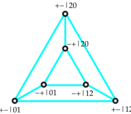
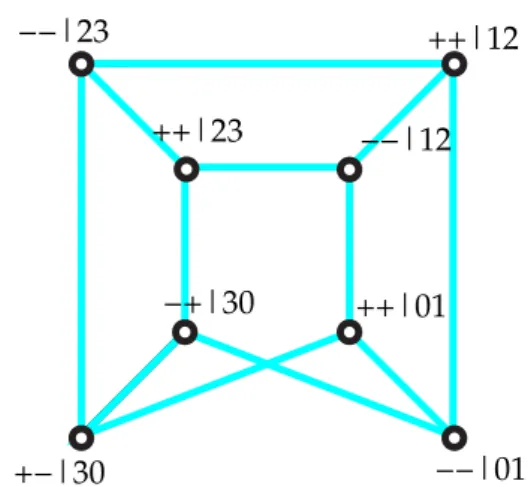
2.5 Then-cycle. . . 53
2.5.1 Quantum violations . . . 56
2.5.2 The CHSH inequality . . . 57
2.5.3 The Klyachko inequality. . . 58
2.6 Boole inequalities as graphs . . . 58
2.6.1 Tsirelson bounds for then-cycle . . . 61
2.7 State-independent Boole inequalities . . . 61
2.7.1 A Boole inequality from the18-projector proof by Ca-bello, Estebaranz, and García-Alcaine . . . 62
2.7.2 A Boole inequality from Yu and Oh’s13-projector proof 62 2.7.3 A Boole inequality from the Peres-Mermin square . . . 62
Conclusion 64
A The Bell-Mermin model 65
In this thesis we explore the question: “what’s strange about quantum mech-anics?”
This exploration is divided in two parts: in the first, we prove that there is in fact something strange about quantum mechanics, by showing that it is not possible to conciliate quantum theory with various different definitions of what should be a “normal” theory, that is, a theory that respects our classical intuition. In the second part, our objective is to describe precisely which parts of quantum mechanics are “non-classical”. For that, we define a “classical” theory as a noncontextual ontological theory, and the “non-classical” parts of quantum mechanics as being the probability distributions that a ontological noncontextual theory cannot reproduce. Exploring this formalism, we find a new family of inequalities that characterize “non-classicality”.
Nessa dissertação exploramos a questão: “o que há de estranho em mecânica quântica?”
Essa exploração se divide em duas partes: na primeira, provamos que de fato há algo estranho em mecânica quântica, mostrando que não é pos-sível conciliar o formalismo quântico com várias definições diferentes do que seria uma teoria “normal”, isto é, que respeite nossa intuição clássica sobre o mundo. Na segunda parte, nosso objetivo é descrever precisamente quais partes da mecânica quântica são “não-clássicas”. Para isso, definimos uma teoria “clássica” como uma teoria ontológica não-contextual, e as partes “não-clássicas” da mecânica quântica como sendo as distribuições de probabilidade que uma teoria ontológica não-contextual não consegue reproduzir. Explor-ando esse formalismo, encontramos uma nova família de desigualdades que caracterizam essa “não-classicalidade”.
Quantum mechanics is magic Daniel Greenberger
This thesis is meant to explore the question posed by Chris Fuchs: what is “Zing!” [1]? What is the property of quantum mechanics which is essentially quantum, absent from any classical theory? Contrary to the goals of Chris Fuchs, our exploration is operationalist rather than axiomatic: our “Zing!” is not a deep axiom that reveals the essence of quantum theory, but rather logically connected sets of probability distributions that cannot be reproduced by any classical theory. Although finding his axiom would be nice, we feel that our approach is more useful, as these sets of probability distributions are the resources needed forquantum magic: quantum computing and quantum key distribution.
This is emphatically not a historical account of the subject: these are plentiful, and another one is unnecessary. Therefore, we shall try to keep references to the great works of von Neumann, Bell, Kochen, and Specker to a bare minimum, while emphasising the newer1works of Abramsky, Busch, Cabello, Hardy, Pitowsky, and Spekkens. The sole exception shall be the work of George Boole, that although very old is still very unknown.
Given a general picture of my motivations and goals, let me now give a more detailed account of the structure of this thesis.
Chapter1presents introductory material2 on the question “is quantum mechanics really different from ‘classical’ theories?”. It begins by capturing some notions of classicality within the framework of ontological theories; then this question is made more precise as “is there an ontological embedding of quantum theory?”.
The chapter proceeds by detailing specific ontological models, and showing which problems arise in trying to reproduce the results of quantum mechanics within them. These problems are then understood as their failure to respect noncontextuality, a notion that we argue to be fundamental in defining clas-sicality. After giving a precise definition of noncontextuality, we proceed to prove Spekkens’ theorem of the impossibility of embedding quantum theory within a preparation noncontextual ontological model.
1As a result, the median year of publishing of our references is2002.
2The reader that is already well-acquainted with the subject (or a mathematician) may find it better to skip it.
We proceed then to revisit our assumptions, and try to find whether a less ambitious notion of classicality can embed quantum theory. To do that, we revisit the historical theorems of von Neumann and Gleason, culminating with the recent version of Busch. In each of their frameworks, a “classical” formulation of quantum mechanics is again ruled out.
The next stop is the famous theorem of Kochen and Specker, that uses the weakest assumptions yet. We present three recent versions of it, by Cabelloet al., Yu and Oh, and Peres and Mermin, that are considerable simplifications of the original proof.
The chapter concludes by presenting a recent theorem of Hardy, that “any ontological embedding of quantum theory is very uncomfortable”, and two specific contextual ontological embeddings of quantum theory.
Our conclusion is then that any reasonable ontological embedding of quantum theory is impossible; therefore thereissomething more in quantum mechanics that classical theories cannot quite capture. Chapter 2 is then dedicated to detail what this something is.
We begin by constructing our final definition of noncontextuality. Based on the recent work of Abramsky and Brandenburger, we show that the Fine theorem admits a natural generalization that applies to any set of observables, without regard to spatial separation. This generalization in its turn motivates a definition of noncontextuality that is a natural generalization of the definition of locality, with mostly the same mathematical structure – this allows us to consider generalizations of Bell inequalities that test noncontextuality instead of locality. Interestingly, this “new” definition was already implicit in the ancient works of Boole (and in the more recent works by Pitowsky), which motivates us to call these generalized Bell inequalitiesBooleinequalities.
The purpose of this part of the thesis is only to establish notation, not to teach quantum mechanics to anyone. If one needs such an introduction, we recommend the excellent book of Michael Nielsen and Isaac Chuang [2].
We say that an operator A is self-adjoint, i.e., A = A∗, if hφ|Aψi =
hAφ|ψi=hφ|A|ψifor all|φi,|ψi. We shall only deal with finite-dimensional operators. The set of all self-ajoint operators isO(H).
A quantum-mechanical observable is a self-adjoint operator.
We say that an operatorAis positive,i.e.,A≥0, ifhψ|A|ψi ≥0 for all|ψi. A quantum stateρis a positive operator such that 0≤trρ≤1 [3]. Since we shall have no use for states such that trρ<1, we can omit the normalization of our quantum states without ambiguity. The set of all quantum states isD(H). A pure quantum state is an extremal point ofD(H), a rank-one projectorψ.
The vector of a pure quantum state will be denoted by|ψi, and the vectors are connected to the projectors by
ψ=|ψihψ|. The set of all pure states isPH.
An effectEis a positive operator smaller than identity,i.e., 0≤E≤1. The
set of all effects isE(H). A set of effects{Ei}such that∑iEi =1describes a
measurement3and is called a POVM.
A projectorΠis a self-adjoint operator such that Π2=Π. The set of all projectors isP(H). A set of projectors{Πi}such that∑iΠi =1 describes
a measurement and is called a PVM. Note that a PVM is a special case of a POVM.
The Born rule is the quantum mechanical rule for associating measurement probabilities with states and effects. We say that
p(i|ρ,E) =trρEi.
3Except for the post-measurement state.
Ontological embeddings of
quantum theory
Classical measurements reveal information. Quantum measurements produce information.
Marcelo Terra Cunha
The quest for embedding quantum mechanics in a “classical” theory is almost as old as quantum theory itself. People were disturbed with the role of measurement in the theory, particularly with its intrinsic randomness and non-repeatability. So they tried to explain away these features as emergent, rather than fundamental, as if they appeared because of a lack of control and understanding of a more refined theory, that would describe the “deeper” physics behind quantum phenomena. We call this refined theory anontological theory.
But despite being familiar, the words “classical” and “ontological” have very fuzzy meanings. In the next section we shall pin them down and clarify them.
1
.
1
What is an ontological theory?
The first ontological models that appeared tried to “solve” the problem of non-determinism. They postulated thatψwas not the real state of nature, but
rather some kind of shadow of it. So they postulated that therewasa real state, an ontic state1, calledλ, that if known would render all measurement outcomes deterministic. That is, given a PVM2M={M
k}, the probability of
outcomekgivenλwould be either 0 or 1, that is, we can define a response
function
ξk|M:Λ→ {0, 1},
1The reader that is well-acquainted with the subject might be wondering when the expression “hidden-variable” will appear. Well, it won’t.
2Even the most determined determinist can’t hope for a POVM to be deterministic. We’ll explain why in a while.
such that ξk|M(λ) is the probability of outcomek. Here, Λis any space in
which our ontic statesλare defined, and to account for the fact that∑kMk =1,
we require that ∑kξk|M(λ) = 1 for all λ. This is just the requirement that
some outcome must occur in a measurement.
Then thesubjectiveindeterminism of quantum theory would be recovered by the ignorance of which ontic states were really present in a experiment. That is, a quantum stateψwould determine a probability distributionµψ(λ)
overΛ. This property can be thought of as “you were trying to generate state
ψ, but you ended up generating an ensemble of ontic states µψ(λ)”. As in
quantum (and classical) mechanics, we shall call the ensembleµψ(λ)itself a
state, while reserving the term pure ontic state for the individualλ, which
can of course be represented as an ensemble with aδdistribution.
Of course, we want this subjective indeterminism to agree with the predic-tions of quantum mechanics, so
p(k|ψ,M) =
Z
Λdλ µψ(λ)ξk|M(λ) =trψMk. (1.1)
1
.
1
.
1
On mixed states and POVMs
The early literature of ontological theories did not do this separation between states and measurements3[4,5]; instead they tried to define a deterministic value functionv(Mk,ψ,λ)that would answer with certainty the outcome of
an experiment, given the quantum state and the ontic state, and recover the quantum statistics by averaging overλ. This is quite problematic, since it can
only describe models in whichψitself has an ontic status4; it therefore can
never describe experiments where the quantum state is explicitly epistemic, e.g., a mixed state. For instance, let’s say we have two pure states ψ and φ with different deterministic outcomes v(Mk,ψ,λ) andv(Mk,φ,λ). Then
if I prepare state ψ with probability p or stateφ with probability (1−p), corresponding to the mixed stateρ= pψ+ (1−p)φ, the outcome must be
v(Mk,ρ,λ) =pv(Mk,ψ,λ) + (1−p)v(Mk,φ,λ),
which is neither 0 nor 1 for non-trivialp, a contradiction.
Using probability distributions like we do, this can be accommodated in a very natural manner:
Lemma 1. If one prepares the quantum states ψi with probabilities pi, then the
corresponding ontic state is
µ(pi,ψi)(λ) =
∑
ipiµψi(λ)
Proof. Quantum mechanics tells us that p(k|(pi,ψi),M) = ∑ipip(k|ψi,M).
Writing these probabilities ontologically, we have5 Z
Λµ(pi,ψi)ξk|M=
∑
i pi ZΛµψiξk|M.
3With the honourable exception of the Kochen-Specker model, discussed in section1.3.1. 4See section1.3for further discussion of this point.
Sinceξk|Mis positive and arbitrary, this implies that
µ(pi,ψi)(λ) =
∑
ipiµψi(λ).
Note that this same rule is used to describe convex combinations of states in quantum and classical mechanics.
The issue with POVMs is similar: one can implement the POVM
E={p|0ih0|,p|1ih1|,(1−p)|+ih+|,(1−p)|−ih−|}
simply by measuring the PVM M ={|0ih0|,|1ih1|} with probabilityp and the PVMN={|+ih+|,|−ih−|}with probability 1−p[6]; we must have then
ξ0|E(λ) = pξ0|M(λ), which is obviously not deterministic. We must accept,
then, that for these kinds of “mixed” POVMs6the response functions must be modified to
ξk|E:Λ→[0, 1],
that is, allowing the whole interval[0, 1]as image.
For “pure” POVMs, this argument does not apply, and we can not decide a prioriwhether to demand them to be deterministic. In fact, it is fruitful to allow even PVMs to be objectively non-deterministic7, so we shall not exclude this possibility.
The most general case is, therefore,
p(k|ρ,E) =
Z
Λdλµρ(λ)ξk|E(λ) =trρEk, (1.2)
and this is what an ontological theory should strive to reproduce, only falling back to pure states and PVMs when unavoidable.
1
.
2
Ontological models
With the definitions given in the previous section, it is already possible to construct some examples of ontological theories, to examine their features in a more concrete manner.
1
.
2
.
1
The naïve ontology
If we allow an ontological model to have objective non-determinism, what we gain in relation to quantum mechanics? Not much, actually. This onto-logical model is so similar to quantum mechanics that it can be confounded with a naïve interpretation of it, that ascribes ontological status to the pure states. Nevertheless, it is quite useful to examine meticulously this ontological
6Following [6], we are calling “mixed” the POVMs that can be written as a convex combination of different POVMs, and “pure” those who can’t.
model, to be aware of the problems that such a naïve interpretation has. This particular model was first proposed by [7], and further explored in [8].
In this model, we are considering the pure statesψto be the ontic statesλ,
so we identify the ontic state spaceΛwithPH, and define
µψ(λ) =δ(λ−ψ).
The response function is then
ξk|E(λ) =trλEk,
and we recover the results of quantum mechanics by
p(k|ψ,E) =
Z
Λdλ δ(λ−ψ)trλEk =trψEk.
We can see, then, that mathematically this ontological model is quite trivial. One interesting thing to examine, though, is the representation of mixed states in this formalism. Following lemma1, we see that
ρ=
∑
i
piψi 7→ µρ(λ) =
∑
i
piδ(λ−ψi),
which trivially reproduces the required quantum statistics. The problem with this approach, however, is that the ontic stateµρ(λ)depends on which
convex decomposition of ρ we chose to use. This makes the the notation µρ suspect, since it should actually beµ(pi,ψi), and blatantly violates theC∗
-algebraic definition of state [9], that requires that states that gives rises to the same statistics to have the same mathematical representation. We call this (unwanted) feature preparation contextuality, which we shall define more carefully in section1.4.
Remember that it is common for beginners to be surprised by the fact that it is impossible to know which convex combination was actually used to construct a given density matrix. Regarding the pure states as ontological, this feeling becomes quite natural, since the mystery is why should the state
µ(pi,ψi)give the same statistics as the stateµ(qi,φi)when∑ipiψi=∑iqiφi.
To solve this problem, one might be tempted to ignore common sense (and lemma1) and ascribe ontological status to mixed states, identifyingΛwith
D(H)instead ofPH; then the ontic states would be just
µρ(λ) =δ(λ−ρ),
relieving us of the basis-dependence. But this is in fact a terrible idea, since one can always write a mixed stateρas a convex combination of two different
statesσ0andσ1, as
ρ=pσ0+ (1−p)σ1.
If you want to regard every mixed state as ontological, you have, by lemma1,
δ(λ−ρ) =pδ(λ−σ0) + (1−p)δ(λ−σ1),
One can now begin to suspect that it is not possible to avoid preparation contextuality; this will be proved in section1.5. For now, we see that even the most humble ontological model, that does not even provide determinism, already has some very undesirable features. It would be a question then if a deterministic ontological model is even possible; fortunately this question was answered a long time ago in the positive. We shall see how in the next subsection.
1
.
2
.
2
Constructing a deterministic ontological model
In1964, Bell had an idea on how to make a deterministic ontological model [4]: hide the quantum mechanical probability of an outcome in the measure of the set of ontic states associated to that outcome. I shall present here a modified version of his model that makes this point quite clear.
This model can describe in a deterministic way the measurement of a one-qubit PVMΠ={Π0,Π1}. The ontic space isΛ=PH ×[0, 1], with ontic variableλ= (λψ,λx). The ontic state of a given quantum stateψis
µψ(λψ,λx) =δ(λψ−ψ),
and the response functions8are
ξ0|Π(λψ,λx) =Θ(trλψΠ0−λx)
ξ1|Π(λψ,λx) =1−ξ0|Π(λψ,λx),
whereΘis the Heaviside step function defined by
Θ(x) = (
1 ifx≥0, 0 ifx<0.
One then recovers quantum statistics by uniform averaging over the ontic space:
p(0|ψ,Π) = Z
Λµψξ0|Π
=
Z
Λdλψdλxδ(λψ−ψ)
Θ(trλψΠ0−λx)
=
Z 1
0 dλx
Θ(trψΠ0−λx)
=
Z trψΠ0
0 dλx=trψΠ0
The reader might have noticed that although the model claims to only work for a qubit, the mathematical formalism does not make any reference to this, and one might be tempted to think that it actually works for any two-outcome PVM. The fact that it does not work is more subtle, and we shall see why in section1.7.
8Note that the response functions depend explicitly on the label of the projectors, so it would be desirable to set a consistent ordering convention to avoid giving different results to
1
.
3
ψ
-ontic and
ψ
-epistemic models
Both models presented in the previous section share a common feature: the quantum state has an ontological status. Either the ontic state is the quantum state itself, like in the naïve model, or it is the quantum state supplemented by real number in the unit interval, as in the Bell model. In both cases, knowing the (pure) ontic stateλof the system is enough to determine uniquely the
(pure) quantum state that was prepared. These kind of models are called9
ψ-ontic, and have the equivalent but more operational definition:
Definition2. An ontological model isψ-ontic if for different quantum statesφand
ψthe ontic states have disjoint support, i.e.,
φ6=ψ ⇒ µφ(λ)µψ(λ) =0 ∀λ
To motivate this definition it might be useful to make an analogy with classical mechanics: in it, an ontic state is a point in phase space, and ontic properties of it (like energy, momentum) are functions of the phase space point. Likewise, anything that is uniquely determined by the ontic state in an ontological theory should be regarded as ontic itself, as a change in it requires a change of the underlying ontic states. As the quantum state is uniquely determined by the ontic state inψ-ontic models, it has to be regarded as ontic,
as it is not possible to change it without changing the underlying ontic states. Apart from conceptual clarity, a reason to make this definition is that it is easy to see thatψ-ontic models necessarily require instant transfer of
informa-tion10. In the first case, whereψis the whole ontic state, it suffices to consider a measurement in an entangled state: Alice and Bob share|φ+i=|00i+|11i and are spatially separated, Alice then measures the PVM{|0ih0|,|1ih1|}and obtains, e.g., the result 0. Bob’s state then changes instantly from1 to|0i,
violating causality. Of course, ifψis not the whole ontic state, there is no
need for a violation of causality: λcan tell us that the state of Bob’s system
actually was|0iall along, and so the ontic state does not change during the measurement.
To deal with this case, we need theeprgedankenexperiment11[13]: consider that Alice can also measure the PVM{|+ih+|,|−ih−|}; then after her meas-urement Bob’s state will belong to the set{|0i,|1i}if she measures the first PVM, or to the set{|+i,|−i}if Alice measures the second PVM. Even if the results of any given measurement can be predetermined byλ, it cannot tell
whichmeasurement was made12. Since Bob’s quantum state does depend on which measurement was made (since the four possibilities are different), the formalism needs again instant transfer of information.
Another way to avoid the violation of causality is to say thatψis not ontic,
but merely the representation of Alice’s knowledge of reality,i.e., epistemic.
9The concept of ontic and epistemic states was first introduced in [10], and further formalized in [8,11]. A nice discussion of these concepts can be found in [12].
10Only in the formalism, of course; if they displayed an observable violation of causality that would be a contradiction with quantum mechanics.
11The version presented here is Einstein’s version, reproduced in [8].
Then what changed after the measurement was actually just what Alice knew about Bob’s state, which is in fact a quite reasonable proposition. But this amounts to give upψ-ontic models in favour ofψ-epistemic ones13:
Definition3. An ontological model isψ-epistemic if it is notψ-ontic.
Again, an analogy with classical mechanics might be useful: the classical mixed state is a probability distribution over the phase space, and it is in-terpreted as epistemic, as it is merely an ignorance about which is the real phase space point that the system occupies. This is only possible as there is no restriction about the overlaps of different mixed states,i.e., the same phase space point can belong to numerous different mixed states. Notice that this definition is quite weak compared to the classical case: it only requires that there is one pairφ,ψwhose ontic statesµφandµψshare a singleλin their
support.
The obvious question to ask: is there aψ-epistemic model?
1
.
3
.
1
The Kochen-Specker model
Even before this question was raised, it was already answered by Simon Kochen and Ernst Specker [14], by the ontological model they constructed as a counterexample to von Neumann’s theorem [15]. It seems that the authors were trying to make a model that was somewhat physically plausible, and ended up making aψ-epistemic model. We presented it here as rendered in
[8].
The ontic spaceΛis the unit sphereS2, and we shall use the Bloch vectors ˆ
ψand ˆφto represent a pure stateψand a measurement projectorφinS2as well, defined via the isomorphismψ= 12(1+ψˆ·σ). The ontic state is then
µψ(λ) = 1
πΘ(ψˆ·λ)ψˆ·λ,
making the model clearlyψ-epistemic, since the only states that do not overlap are orthogonal states. The response function is given by
ξφ(λ) =Θ(φˆ·λ).
To recover the quantum statistics, notice that each ofµψ andξφhas as support
an hemisphere centred in ˆψand ˆφ, so their intersection defines a spherical
lune. To take advantage of this, let’s choose coordinates such that ˆψand ˆφ
lie in the equator ofS2, so that ˆψ= (cosψ, sinψ, 0), ˆφ= (cosφ, sinφ, 0), and
λ= (sinθcosϕ, sinθsinϕ, cosθ). We have then
p(φ|ψ) =
Z Λdλ
1
πΘ(ψˆ·λ)ψˆ·λΘ(φˆ·λ)
= 1
π
Z
S2d
Ω Θ(sinθcos(ϕ−ψ))sinθcos(ϕ−ψ)Θ(sinθcos(ϕ−φ))
= 1
π
Z π
0 dθsin 2θZ 2π
0 dϕΘ(cos(ϕ−ψ))cos(ϕ−ψ)Θ(cos(ϕ−φ)) = 1
2 Z ψ+π2
φ−π
2
dϕcos(ϕ−ψ)
= 1
2(1−sin(φ−ψ−π/2)) = 1
2(1+cos(φ−ψ)) =trψφ.
This model does seem to be the most “natural” of the ontological models yet considered, and there have even been attempts to understand it physically [16]. In this same article, Terry Rudolph explores extensions of the Kochen-Specker model to higher dimensions, but fails to precisely reproduce quantum mechanics with them. Albeit it wasψ-epistemic model for higher dimensions
has since then been found (we discuss it in section1.9.2), it does not have the simplicity of the Kochen-Specker model, and so it would be unfair to call it an extension of it.
1
.
3
.
2
Two theorems on
ψ
-epistemic models
We can see, then, thatψ-epistemic models are desirable and can actually be
constructed. There are, however, two theorems that say that any such model, if it exists, has to be very unnatural. They are both based on the following idea:
Lemma4. If there are quantum statesψiand measurements Eisuch thattrψiEi =0
∀i, then there can be noλ0in the support of allµψi.
Proof. If these conditions are satisfied, then it must be true that
Z
Λdλ µψi(λ)ξi|E(λ) =0,
and therefore thatξi|E(λ) =0 for allλin the support ofµψi. If there is aλ0in
the support of all theµψi, making the modelψ-epistemic, then∑iξi|E(λ0) =0,
an absurd, since in the definition of the response functions we require that ∑iξi|E(λ) =1 for allλ.
Of course, if we could prove that foranypair of states the hypothesis of the lemma are satisfied, we would have proven that no ψ-epistemic model
Lemma5. If there are quantum statesψ0,ψ1and measurements E,1−E such that
trψ0E=trψ1(1−E) =0, thenψ0ψ1=0
Proof. trψ1(1−E) =0 ⇒ trψ1E= 1, so the support ofψ1 is contained
in the support ofE. But trψ0E=0 implies that the supports ofψ0and Eare
disjoint, and therefore the supports ofψ0andψ1are disjoint, soψ0ψ1=0
Instead, the two theorems we shall present consider larger families: the first considers families of three states to show that there are non-trivial examples, and the second argues that the existence of some specific families implies that anyψ-epistemic model must be very unnatural.
Theorem6(Caves, Fuchs, Shack [17]). If the convex hull of a family of statesψi
contains1/d, where d is the Hilbert space dimension, then there can be noλ0in the
common support of allµψi.
Proof. For any state ψi, it is true that trψi(1−ψi) =0. If we can find coeffi-cientsαi such that{αi(1−ψi)}is a POVM, then lemma4applies and we’re done. What we need is
∑
i
αi(1−ψi) =1,
for αi ≥0. Taking the trace on both sides we get that ∑iαi = d
d−1. Simple
algebra then shows us that
∑
i
d−1 d αiψi =
1 d1.
This theorem was first proven in [17], with a different objective. While it does not exclude ψ-epistemic models, it shows there are a wide variety of
families of states that can’t have an overlap. If the number of states is three, there are already examples in any dimension where they are not orthogonal; see equations (1.6) for an example.
The next theorem needs the following (very natural, in the author’s opin-ion) assumption about the composition of different systems:
Assumption1. If two quantum states φandψare prepared independently, such that their joint state isφ⊗ψ, then the corresponding ontic state for the joint system isµφ⊗ψ(λA,λB) =µφ(λA)µψ(λB).
Theorem7(Pusey, Barret, Rudolph14[18]). Given assumption1, noψ-epistemic ontological model of quantum mechanics is possible.
Proof. Consider the four quantum statesφ0⊗φ0,φ0⊗φ1,φ1⊗φ0, andφ1⊗φ1.
If there is aλ0in the support ofµφ0 andµφ1, then(λ0,λ0)is in the support of
all fourµφi(λ′)µφj(λ′′). If there is a POVM
Eij such that trφi⊗φjEij =0,
then lemma4applies and we’re done.
Consider now the particular case|φ0i=|0iand|φ1i=|+i. Then ifEijis
the projector onto Eij
=|φiφ⊥j i+ φ⊥i φj
, it is easy to see that
trφi⊗φjEij =φiφj
Eij
=0,
and it is also easy (but tedious) to check that∑ijEij =1. Unfortunately, this
simple strategy only works for this pair of states, and states with smaller overlap require measurements on a larger number of parts. For the proof of the general case, see the original article [18].
This theorem has two immediate corollaries:
Corollary8. Any ontological model of quantum mechanics must violate causality.
One only has to notice that since the theorem excludesψ-epistemic models,
we’re left withψ-ontic ones. And we have shown that those violate causality
in the beginning of this section.
Corollary9. The ontic state spaceΛis uncountable.
In aψ-ontic model there is an injection ofP(H)onto Λ. SinceP(H)is uncountable,Λmust be uncountable. In fact, even if without assumption1 we can still prove thatΛis infinite; we shall do this in section1.8.
The obvious question that this theorem raises is: can we do away with assumption1and prove once and for all thatψ-epistemic models are always
impossible? The existence of the Kochen-Specker model already hints that at least some weaker assumption is needed, since it is abona fide ψ-epistemic
model. Of course, its existence does not contradict the theorem, since it only forbids models for dimension4or greater. In fact, soon after the Pusey-Barret-Rudolph was published, some of the same authors showed that without assumption1they could make aψ-epistemic model for a quantum system of
any dimension. We shall describe this model in section1.9.2.
This theorem already hints of a theme that shall be recurrent in the search for ontological models: we can in fact make ontological models for quantum theory, and in fact we can make them almost in any way that we like, but there’s a price to pay: the various aspects of the model become more and more intertwined. We can’t really talk of independent quantum systems, separation between state and experiment, nor even (as we shall see in the next section) talk about a measurement outcome without talking about the whole experiment. Of course, this bodes very badly for the idea of ontological models: in the extreme limit of this interdependence our ontological model only lists possible experiments and their results, without ever trying to make sense of them in a simpler and more general theory. A model like this wouldn’t be falsifiable by its very nature, but precisely because of this it is a perversion of the scientific method [19], and should therefore be rejected on methodological grounds.
evidence against the possibility of a reasonable ontological model, since they were conceived only as proofs of principle, without any inspiration from physical grounds.
1
.
4
Contextuality
One should contrast the state of research into contextuality to the state of research into nonlocality. It is quite clear that nonlocality has a better status: it was subjected to experimental tests much earlier15, and also had its potential as a resource for practical applications recognized much earlier16
This state of affairs has many causes, which certainly includes the intuitive appeal of nonlocality via its relation with relativity, but I’d like to focus in a more formal one: the definitions of nonlocality and contextuality. Right in the first paper about nonlocality, John Bell [24] already gave a clear operational definition of nonlocality, that was not dependent on quantum theory, but instead only on a general probabilistic framework. By contrast, the first defin-ition of contextuality, also due to John Bell17, was very specific to quantum theory, and was not at all operational:
Definition10(Bell’s contextuality). We say that an ontological model for quantum theory is noncontextual if the response function associated to the outcome k of a PVM M={Πk}, i.e.,ξk|M(λ)depends only onΠkand not on the whole M.
This definition also lacks conceptual clarity: John Bell even thought that it was reasonable for a physical theory to be contextual [4]:
The result of an observation may reasonably depend not only on the state of the system (including hidden variable) but also on the complete disposition of the apparatus.
But one consequence of contextuality is precisely the violation of causality that he abhorred: consider, for instance, the PVM
M={Π0⊗1,Π1⊗1,1⊗Π0,1⊗Π1}.
If the real resultξ0|M(λ), associated with the projectorΠ0⊗1, depends on
whether the other side of the PVM is1⊗Π0,1⊗Π1or1⊗Π′0,1⊗Π′1, then the apparatuses must always be able to communicate their arrangement to each other, even when the choice of arrangement is made with a space-like separation, which is of course absurd. This settles the question about ontological models of independent quantum systems. But what about single systems? Is there any unacceptable consequence of contextuality for them?
Yes! It also implies on a violation of causality. As put by Asher Peres and Amiran Ron [26]:
151972[20], in contrast with2000[21]. 161991[22],versus2000[23].
More generally, if [A,B] = [A,C] = 0 but [B,C] 6= 0, suppose that we measureAfirst and only a later time decide whether to measure Bor C or none of them. How can the outcome of the measurementAdepend on this future decision?
Furthermore, this whole story about communicating apparatuses is quite queer, even when it is not a violation of causality. After all, all the evidence we have is that the measurement of commuting observables does not affect each other, and an ontological theory that requires this kind of communication would be very weird indeed. Another problem is that this communication could affect only the individual measurementsξi|M(λ), and must never be
detectable in the quantum experiments we do. To postulate this kind of “cryptocontextuality”18seems very unscientific: we would be making a theory
which is about precisely what wecan’tmeasure.
Another way to think about the weirdness of a contextual model is op-erationally: imagine that you are an experimentalist that has implemented an apparatus that can differentiate between the ground state and the excited states of a many-level atom. You try it hard, repeat your experiment a lot of times, with different input states, gather the statistics, and is confident that your apparatus is quite trustworthy; you now want to teach a friend experi-mentalist how to build a similar apparatus. Quite simple, isn’t it? You just tell him how you did, ask him to gather statistics, and compare with yours: if the statistics match, you’ve implemented the same experiment. Except it isn’t so if your physical theory is contextual: the statistics of the projectorΠ0(the projector onto the ground state) are not enough to determine the results of the experiment, since according to definition10the real resultsξ0|Π(λ)depend on the rest of the (unmeasured) projectors; and these are not only the higher energy levels of the atom, but can in principle include any environmental data, such as the apparatus’ mass, the local weather, whether Virgo is ascendant. . .
In this way, we are rendered incapable of comparing experiments and establishing patterns, the very foundation of our scientific method. Notice the strong parallel between this discussion and the definitions of state and observable in theC∗-algebraic axiomatization done by Franco Strocchi [9]. This motivates a new definition of contextuality, due to Spekkens [11], that takes into account these arguments:
A noncontextual ontological model of an operational theory is one wherein if two experimental procedures are operationally equival-ent, then they have equivalent representations in the ontological model.
Within this reasoning, it becomes sufficient to have equivalent statistics to be able to identify different experiments, and we are able again to do science. But a definition that uses only words is quite imprecise, and we should codify it in order to avoid misinterpretations:
Definition 11 (Spekkens’ contextuality). Let p(k|P,M) be the probability of obtaining the outcome k when doing the measurement M on a state prepared via procedure P. Then we say that an ontological model of an operational theory is measurement noncontextual if
p(k|P,M) =p(k|P,M′) ∀P ⇒ M=M′. (1.3) Analogously, we say that an ontological model of an operational theory is preparation noncontextual if
p(k|P,M) =p(k|P′,M) ∀M ⇒ P=P′. (1.4) The central idea is simple: if measurements M and M′ give the same statistics for every preparation procedureP, then we must say that they are in fact the same measurement, with equivalent mathematical representation, and if preparation procedures P and P′ give the same statistics for every measurement M, then we must say that they are in fact the same preparation procedure, with equivalent mathematical representation.
Note that this definition improves on Bell’s definition by removing any explicit reference to quantum theory, talking about only an “operational theory”, i.e., a theory in which we can talk about preparation procedures, measurements, and probabilities. However, this is still not the definition we’re looking for. We want to be able to say whether a given probability distribution is contextual or not, as we do with the definition of nonlocality. This we shall do in the next chapter; for this one, this definition is good enough.
We want to specialize this definition to ontological models of quantum theory, as a matter of convenience, since that’s all we’ll be talking about. Note that in quantum theory p(k|P,M) = trρMk is completely defined by
the measurement operator Mk and the quantum state ρ, so that’s all our
ontological model can take into account. More precisely
Definition12. We say that an ontological model of quantum theory is measurement noncontextual if
ξk|M(λ) =ξMk(λ),
that is, if the response function associated to the outcome k of a measurement M de-pends only on the measurement operator Mk. Analogously, we say that an ontological
model of quantum theory is preparation noncontextual if
µP(λ) =µρ(λ),
that is, if the ontic state associated to the preparation procedure P depends only on the quantum stateρthat is prepared.
What else could the ontic stateµP(λ)possibly depend on? Well, in the ontological models we discussed in sections1.2.1and1.2.2it depended on the “true” basis ofρ, making these states preparation contextual. It could also
depend on the “true” purification ofρ, or really anything that one might deem
as do the ontological models discussed on section1.9.2, but it could also be anything, such as the colour of the measurement apparatus, the latitude and longitude of the laboratory where the experiment is performed, etc.
One final remark: if quantum theory were an ontological model of itself then definition11(and12) would imply that it isnot contextual, since it is trivial to prove that
trρMk=trρMk′ ∀ρ ⇒Mk=M′k
and
trρMk =trσMk ∀Mk ⇒ρ=σ.
Since it is not, the oft-heard claim that “quantum mechanics is contextual” is just meaningless. What one probably means with it is that any ontological model of quantum theory must be contextual, repeating a situation that happen in the area of nonlocality: quantum mechanics is obviously a local theory, in the relativistic sense, but any ontological model of quantum theory must be nonlocal, leading to the meaningless sentence “quantum mechanics is nonlocal”.
1
.
5
Contextuality for preparation procedures
In this section we shall show that it is not possible to construct a preparation noncontextual ontological model of quantum theory [11]. This is not the con-flict with quantum theory usually discussed, but we feel that it is appropriate to begin with it for three reasons:
1. It is independent of assumptions on determinism
2. It is simple
3. It is novel
To begin, we’ll need to prove a simple lemma about how orthogonal states are represented in the ontic spaceΛ. We’ll see that the possibility of distinguishing orthogonal states with certainty by a single-shot measurement implies that their representations in the ontic space must have disjoint support.
Lemma13. If two quantum statesρandσare orthogonal then the corresponding ontic statesµρandµσ have disjoint support:
ρσ=0 ⇒ µρ(λ)µσ(λ) =0 ∀λ
Proof. Ifρandσare orthogonal, then they can be distinguished with certainty
in a single-shot measurement. To construct one such measurement, note that the supports ofρandσmust be orthogonal, and letΠρbe the projector onto the support ofρ. Then
Writing these measurements ontologically, we have Z
ΛµρξΠρ =1 and Z
ΛµσξΠρ =0,
soξΠρ(λ) =1 for allλin the support ofµρ, andξΠρ(λ) =0 for allλin the support ofµσ, so the supports ofµρandµσ are disjoint, andµρ(λ)µσ(λ) =0
for allλ.
We will also need the assumption that is violated by all the ontological models discussed so far:
Assumption2(Preparation noncontextuality).
∑
i
piψi =
∑
i
qiφi ⇒ µ(pi,ψi)(λ) =µ(qi,φi)(λ)
With the groundwork laid, we can now state the theorem and prove it.
Theorem14(Spekkens [11]). It is not possible to embed quantum theory into a preparation noncontextual ontological theory.
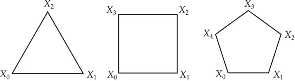
Proof. Letφ,Φ,χ, X,ψ, andΨbe quantum states such that
0=φΦ=χX=ψΨ (1.5a)
1=φ+Φ=χ+X=ψ+Ψ (1.5b)
3
21=φ+χ+ψ=Φ+X+Ψ. (1.5c) That such a family of states exists can be proven by exhibiting an example in dimension2, that can be easily embedded in higher dimensions:
|φi=|0i |Φi=|1i (1.6a)
|χi= 1 2|0i+
√
3
2 |1i |Xi=
√
3 2 |0i −
1
2|1i (1.6b)
|ψi= 1 2|0i −
√
3
2 |1i |Ψi=
√
3 2 |0i+
1
2|1i (1.6c) A nice way to visualize the orthogonality and completeness relations (1.5) is to represent states (1.6) in theσx,σz plane of the Bloch sphere, as done in
figure1.1.
Now we shall use lemmas 1 and 13 together with assumption 2 and relations (1.5) to derive a contradiction. Lemma13together with (1.5a) implies that
µφ(λ)µΦ(λ) =µχ(λ)µX(λ) =µψ(λ)µΨ(λ) =0 ∀λ (1.7)
Lemma1, together with assumption2and relations (1.5b), implies that
µ1 21=
1
2 µφ+µΦ
(1.8a)
= 1
2(µχ+µX) (1.8b) = 1
Figure1.1: Representation of states (1.6) in theσx,σzplane of the Bloch sphere.
The barycenter of antipodal states or states which are connected by a triangle is1/2.
and together with relations (1.5c)
µ1 21=
1
3 µφ+µχ+µψ (1.9a) = 1
3(µΦ+µX+µΨ). (1.9b) We shall conclude the proof by showing that the only simultaneous solu-tion to (1.8), (1.9), and (1.7) is the all-zero solution
µφ(λ) =µΦ(λ) =µχ(λ) =µX(λ) =µψ(λ) =µΨ(λ) =0 ∀λ,
which is absurd, since probability distributions can’t be zero everywhere. The disjointness relations (1.7) imply that for eachλat least one ofµφand
µΦ must be zero, and the same for the other letters. Therefore there are 8 different cases to examine, although only two are essentially different. The first one is whenµφ,µχ, andµψare zero. Then (1.9) implies thatµΦ,µX, and
µΨmust also be zero. The second case is whenµΦ,µχ, andµψare zero. Then
(1.8a) implies thatµ1 21=
1
2µφ, and (1.9a) implies thatµ1 21=
1
3µφ. But the only
solution to 12µφ= 13µφisµφ=0, and we can apply the previous argument to
show that all probability distributions must be zero. The six remaining cases are simply relabellings of these two.
As the above argument applies to everyλ, we have that all probability
1
.
6
Gleason theorems
There are three theorems that I call “Gleason theorems”: von Neumann’s theorem [15], Gleason’s theorem [27] and Busch’s theorem [28]. Of these three, the most famous is certainly Gleason’s19, and that is why I chose to name this section after it. All three theorems share a similar structure: they postulate some properties that a measurementµshould have, and then prove that the
only measurement that satisfies those properties is the quantum mechanical oneµ(A) =trρA. They can be interpreted in two ways:
1. As an axiomatic improvement, by showing that the notion of quantum state and Born’s rule follow from weaker axioms.
2. As excluding deterministic ontological theories, by saying that properties ofµshould be true inanytheory, not only in quantum mechanics. Then one only has to notice that Born’s rule is not deterministic.
If one chooses the first interpretation, all three theorems are perfectly fine, and in fact quite similar. Problems arise, however, if one insists on interpreting them as excluding deterministic ontological theories. Then von Neumann’s theorem becomesfoolish20[5], as its assumptions already excludes a large class of ontological theories, without good reason.
1
.
6
.
1
von Neumann’s theorem
Theorem 15 (von Neumann [15]). Let A,B be self-adjoint operators, and µ :
O(H)→Ra function such that
1. µ(αA) =αµ(A)for realα.
2. µ(A+B) =µ(A) +µ(B)for commuting A,B.
3. µ(A+B) =µ(A) +µ(B)for non-commuting A,B.
4. µ(1) =1
5. µ(A)≥0for positive A.
Then any such function can be written as
µ(Π) =trρΠ,
whereρis a positive operator of unit trace.
Proof. Properties1,2, and3establish thatµis a linear functional onO(H), and by the Riesz lemma can be represented as an inner productµ(A) =trρA. Property 4then implies that ρ has unity trace, as µ(1) = trρ1 = trρ = 1, and property5implies its positivity, since in particular projectors are positive operators, andµ(|ψihψ|) =trρ|ψihψ|=hψ|ρ|ψi ≥0 for allψis the definition
of positivity.
19The most infamous being von Neumann’s. Busch’s theorem is still new.
We can see, then, that the theorem itself is quite simple, and its value resides in the strength of its assumptions, which we shall examine now. The first thing one may notice is that the theorem already makes use of the Hilbert space formalism for the observables, and the fact that the states also follow the same formalism seems almost like a tautology. But this is not the case. Quantum mechanics can already implement this formalism in experiments in a quite successful manner, and one may regard observableAas just a proxy for the experiment that implements it; asµcan be any functiona priori(we don’t even assume it is continuous), there is not limitation in using O(H) as its domain. We shall now proceed to examine the physical content of the assumptions.
Assumption1and2can be interpreted as doing classical post-processing to the data of a single experiment, the measurement of a PVM{Πi}, that we define from the eigendecomposition of A. The multiplication of A by a constant is implemented just by multiplying its eigenvalues by the same constant. To implement the observable A+B corresponding to the sum of commuting operators AandBone notices that they can be diagonalized simultaneously as A = ∑iaiΠi and B = ∑ibiΠi, and so their sum A+B = ∑i(ai+bi)Πi
is just a combination and rescaling of the data coming from theΠioutputs. Assumptions4and5can be justified by the possibility of interpretingµ(Πi) as a probability: probabilities are positive, and some outcome must happen.
The one which is harder to justify is assumption3, sinceA,B, and A+B correspond to different experimental configurations: so the possibility of measuring A+B just by processing the data coming from the PVMs that measure A or B is excluded. Its justification comes from the fact that in quantum mechanics trρ(A+B) =trρA+trρB, and our ontological theory
must reproduce its results. But this is where von Neumann slips, and to make the slip more clear, it’s best to use the ontological notation, the correspondence beingµ(A) =ξA(λ). So assumption3translates to
ξA+B(λ) =ξA(λ) +ξB(λ),
which is clearly overkill, since correspondence with quantum mechanics only requires that
Z
ΛµρξA+B = Z
ΛµρξA+ Z
ΛµρξB,
that is, that the expected values correspond, not the values of the response functions themselves. For instance, in the Bell-Mermin model, discussed in appendixA, we can see that the response function (A.1) is clearly linear with respect to the sum of commuting observables21
as
ξA+B(ψ,λ) =a0+b0+ka+αaksign((a+αa)·(λ+ψˆ))
=a0+b0+|1+α|kaksign(1+α)sign(a·(λ+ψˆ)) =a0+kaksign(a·(λ+ψˆ)) +b0+αkaksign(a·(λ+ψˆ)) =ξA(ψ,λ) +ξB(ψ,λ),
since the values thatξAassumes are the eigenvalues ofA, and eigenvaluesare linear with respect to the sum of commuting observables. Of course, this is not true when the observables do not commute, as we can see in the following example:
ξσx+σz(ψ,λ) =
√
2 sign(λx+ψx+λz+ψz)
6
=sign(λx+ψx) +sign(λz+ψz) =ξσx(ψ,λ) +ξσz(ψ,λ).
Therefore, we must conclude that this assumption is unfounded, and if no justification can be found to it, we must abandon von Neumann’s prohibition of ontological models. We shall see, however, that even if we abandon this assumption, we can still prove a von Neumann-like theorem, valid in a more restricted context: that is Gleason’s theorem. More surprisingly, however, is the fact that this assumptioncanbe justified, by the consideration of POVMs. This realisation is what motivated the proof of Busch’s theorem.
1
.
6
.
2
Gleason’s theorem
Andrew Gleason was not concerned with von Neumann’s theorem, not even with the problem of ontological models for quantum mechanics. His goal was to study the mathematical foundations of quantum mechanics, and to strengthen its axiomatic basis by showing that essentially every measure on a Hilbert space is given by Born’s rule [27]. Its significance to the exclusion of ontological models of quantum mechanics was first noticed by Bell [4], who also remarked that contextual ontological models were not bound by Gleason’s theorem.
Theorem 16 (Gleason [27]). Let H be a separable Hilbert space over C with dimH ≥3, andµ : P(H) → [0, 1] a function such that∑iµ(Πi) = 1 for any PVM{Πi}. Then any such function can be written as
µ(Πi) =trρΠi,
whereρis a positive operator of unity trace.
The proof of this theorem is already well-known, and a bit boring, so we shall omit it. The interested reader may find it in the original work [27], or in the clearer version by Bell [4].
It is easy to see that von Neumann’sµfunctions satisfy all the properties of
“reasonable” von Neumann theorem, with weaker assumptions. Also notice that Gleason’s assumptions are explicitly non-contextual, by assuming that
µ(Πi)is only a function of the projectorΠi, and not of the whole PVM.
1
.
6
.
3
Busch’s theorem
Paul Busch was concerned with the justification of von Neumann’s assumption 3. He noticed that if one measures a POVM {Ei}instead of a PVM, then
it is possible to have in a single experiment two outcomes E0 andE1 that
do not commute22, so it is perfectly natural to demand that µ(E
0+E1) =
µ(E0) +µ(E1), since one can measureE0+E1just by combining the outcomes corresponding to E0 and E1. He then restricted assumption3 to sums of
effects belonging to a single POVM, and was able to derive Born’s rule from it, thus resurrecting von Neumann’s theorem [31]. Later he realized that the form of his theorem was actually closer to Gleason’s than von Neumann’s; to obtain it from Gleason’s one only has to demand∑iµ(Πi) =1 to be true for POVMs, instead of just form PVMs. Interpreted in this way, his theorem is a much stronger version of Gleason’s with a much simpler proof [28].
The proof presented here mostly follows the one presented in [1], with the difference that it does not require the domain ofµto be extended.
Theorem17(Busch [28]). LetHbe a separable Hilbert space over23 Q[i]orC, and
µ:E(H) →[0, 1]a function such that∑iµ(Ei) =1for any POVM{Ei}. Then
any such function can be written as
µ(Ei) =trρEi,
whereρis a positive operator of unity trace.
Proof. The proof begins by noticing thatµis in fact a linear functional onE(H). From that, the Riesz lemma establishes that it can represented as an inner product. Positivity and normalization ofρthen comes from the positivity and
normalization ofµ. We shall first prove the case whereHis over the complex rationals, and later extend the proof to the continuum.
First note that ifEis an effect,1−E is also an effect. Then considering the POVMs {E,1−E}and{E1,E2, . . . ,En,1−E}, where∑iEi = E, we see
that µ(E) = ∑iµ(Ei). Considering the particular case Ei = E/n, we get
that µ(E) = nµ(E/n). On the other hand, if we consider E = mF and Ei = F, we getµ(mF) = mµ(F). Combining these two cases, we see that
µ(m
nE) = mµ(n1E) = mnµ(E), that is, µ(qE) = qµ(E) for q ∈ Q+ whenever
bothqEandEare effects. Wrapping up, we have that
µ(E) =
∑
i
qiµ(Ei)
for rational qi whenever qiEi are effects, so µalready has some restricted
linearity. If we can remove the restriction that qiEi are effects, we get full
linearity onE(H), and that’s what we’ll do now.
22In fact, this happens in all non-trivial POVMs..
23Q[i] is the field extension of the rationals Q with the imaginary number i, Q[i] =
Consider the effects E and F ≤ E. Then E = E−F+F, and µ(E) =
µ(E−F) +µ(F), so µ(E−F) =µ(E)−µ(F). Consider now E,F,G∈ E(H) andp,q∈Q+such thatE=pF−qG, but at least one ofpandqis larger than unity, so pFandqGare not necessarily effects. Without loss of generality, let p≥q. Then 1pE,F, and qpGare all effects, and by the property we just proved,
µ(1qE) =µ(F)−µ(qpG), soµ(E) =pµ(F)−qµ(G)and
µ(E) =
∑
i
qiµ(Ei)
foranyrationalqi, so we have full linearity onE(H). Let then{Ei}d
2
i=1be a
MIC-POVM and, as such, a basis forH. Then any effectEcan be written as E=∑di=21qiEi forqi ∈Q(a moment’s thought will convince you that complex
numbers aren’t allowed). We can now define ρby solving thed2equations trρEi=µ(Ei), and see that
µ(E) =
d2
∑
i=1
qiµ(Ei) = d2
∑
i=1
qitrρEi =tr ρ d2
∑
i=1
qiEi
!
=trρE.
Positivity ofρcomes from considering the case whereEis a one-dimensional projector:
0≤trρE=trρ|ψihψ|=hψ|ρ|ψi. The unity of the trace comes from
1=
∑
i
µ(Ei) =
∑
i
trρEi =tr ρ
∑
iEi
! =trρ.
This completes the proof forQ[i]. To extend it to the continuum, note again that ifE≥F, thenµ(E) =µ(E−F) +µ(F), and soµ(E)≥µ(F). Let thenpi
andqibe sequences of rational numbers tending to the real numberαsuch that
pi≤α≤qi. We have piE≤αE≤qiE, and as such piµ(E)≤µ(αE)≤qiµ(E),
soµ(αE) =αµ(E). From this fact, one can now retrace the proof and see that it also holds forC.
The reason that we decided to highlight the fact that Busch’s theorem holds for Q[i] is that the original Gleason theorem fails for it, hinting that traditional contextuality might have problems dealing with subsets ofC[32,
33]. This feature of Busch’s theorem was first noticed in [34].
1
.
6
.
4
Wrapping up
interested in the question of ontological theories, but in which measures are allowed given the Hilbert space structure of observables, the following counterexample24should suffice:
µψ(φ) =1
2(1+cos(ncos−1(φˆ·ψˆ))), oddn Note that forn=1 this formula is simply Born’s rule.
It is easy to check that
∑
i
µ(Πi) =µψ(φ) +µψ(1−φ)
= 1
2(1+cos(ncos−1(φˆ·ψˆ))) + 1
2(1+cos(ncos−1(φˆ·ψˆ) +π)) = 1
2(1+cos(ncos−1(φˆ·ψˆ))) + 1
2(1−cos(ncos−1(φˆ·ψˆ))) =1,
as required in Gleason’s assumptions.
To see that forn≥3 this formula can’t equal Born’s rule, notice that
trψφ= 1
2(1+φˆ·ψˆ)
only has one root, if considered as a function of the angle cos−1(φˆ·ψˆ), whereas
ourµψ(φ)hasnroots.
1
.
7
The Kochen-Specker theorem
A corollary of the Gleason theorem is that one can’t embed quantum theory in a noncontextual ontological model if dimH ≥ 3, since the Born rule is explicitly noncontextual and non-deterministic; a direct proof of this fact might seem superfluous. But one might not like its assumptions: after all, it already assumes a fair bit of structure that is not quite needed and, more importantly, it needs to assume that the quantum valuationµ(Πi)is defined for a continuous amount of projectors, which of course can never have experimental justification. This was the motivation25 for Simon Kochen and Ernst Specker to develop afiniteproof of noncontextuality, finding an inconsistency in any deterministic assignment of values to a set of experiments realizable in quantum mechanics [14]. Another motivation to present it here is that it proves the claim in section 1.2.2that noncontextual deterministic ontological models can not describe two-outcome PVMs.
In modern parlance, the Kochen-Specker theorem is referred to as a proof of state-independent contextuality, as the logical contradiction found depends only on the structure of quantum observables, and not on the statistics from the measurement of specific states. This situation contrasts, of course, with
24Due to Marcelo Terra Cunha and Rafael Rabelo.

![Figure 1.2: Vectors for the 18-projector proof of the Kochen-Specker theorem. Reproduced from [41] with permission from the author.](https://thumb-eu.123doks.com/thumbv2/123dok_br/15739417.125326/34.892.188.698.186.545/figure-vectors-projector-kochen-specker-theorem-reproduced-permission.webp)
![Figure 1.3: Orthogonality graph for the proof of Yu and Oh. Reproduced from [43] with permission from the authors.](https://thumb-eu.123doks.com/thumbv2/123dok_br/15739417.125326/35.892.193.692.184.606/figure-orthogonality-graph-proof-yu-reproduced-permission-authors.webp)