On the stress investigation at the edges of the fixed elastic semi-strip

(1)

N. Vaysfeld et alii, Frattura ed Integrità Strutturale, 38 (2016) 1-11; DOI: 10.3221/IGF-ESIS.38.01

1

Focussed on Multiaxial Fatigue and Fracture

On the stress investigation at the edges

of the fixed elastic semi-strip

N. Vaysfeld

Odessa Mechnikov University, Institute of Mathematics, Economics and Mechanics vaysfeld@onu.edu.ua

O. Kryvyi

National University «Odessa Maritime Academy» (NU «OMA») krivoy-odessa@ukr.net, kryvyi-od@math.onma.edu.ua

Z. Zhuravlova

Odessa Mechnikov University, Institute of Mathematics, Economics and Mechanics zhuravleva@te.net.ua

ABSTRACT. The stress state of the elastic fixed semi-strip with the regarding

of the singularities at its edge is investigated in the article. The initial boundary problem is reduced to a vector boundary problem in the transformation’s domain by the use of integral Fourier transformation. The one-dimensional vector boundary problem is solved exactly with the help of matrix differential calculations and Green’s matrix apparatus. The problem’s solving was focused at the solving of the singular integral equation (SIE) with the two fixed singularities at the ends of the integration’s interval. The symbol of SIE was constructed and the generalized method of the SIE solving was applied. The stress’ distributions of the semi-strip are investigated.

KEYWORDS. Semi-strip; Vector boundary problem; Singular integral equation;

Fixed singularity.

Citation: Vaysfeld, N., Kryvyi, O., Zhuravlova, Z., On the stress investigation at the edges of the fixed elastic semi-strip, Frattura ed Integrità Strutturale, 38 (2016) 1-11.

Received: 14.04.2016

Accepted: 09.06.2016

Published: 01.10.2016

Copyright: © 2016 This is an open access article under the terms of the CC-BY 4.0, which permits unrestricted use, distribution, and reproduction in any medium, provided the original author and source are credited.

INTRODUCTION

he plain elasticity problems for a semi-strip are important as the model examples for the different engineering applications. So many authors have examined these problems in their works. A short review of the different approaches to the solving of the plane elasticity problems for an elastic semi-strip is given below.

(2)

2

of an infinity system of the algebraic equations. The variation method was used for the analogical problem’s solving in [6-8]. The energetic method was applied to the problem of the semi-strip with the free lateral edges and loaded short edge in [9]. In [10] authors constructed a special system of byorthogonal functions, with the help of which they solved the problem on a semi-strip loading at it’s the short edge. The problem for the semi-strip with the free longitudinal sides was solved with the help of the stress function in [11, 12]. The Laplace’s integral transformation was used for the problem’s solving in [13]. The approach based on the use of Fadle-Papkovich functions was applied in [14-16].

In this paper the method, which was worked out by G. Ya. Popov, was used [17]. Accordingly to it the integral transformations were applied directly to the equilibrium equations and boundary conditions of a problem. It leaded the initial problem to one-dimensional boundary problem in the transformation’s domain. The last one was formulated as the vector boundary valued problem and solved exactly with the apparatuses of the matrix differential calculations and Green’s matrix function [18]. The problem was reduced to the singular integral equation’s solving. Investigation of the signature’s nature of the singular integral equation’s solving was under consideration of many famous scientists. Today the new theories are appeared, which describe the solution’s behavior at the particular points [19]. The investigations of the singularities’ nature for the complex medium are continued [20]. But in most studies the authors did not pay attention to the fixed singularities at the angular points of the semi-strip usually, although these singularities play a main role in the estimation of the stress state. One approach that allows to find and to take such singularities into account was proposed in widely known work [21]. It was used in this paper for the fixed singularities’ consideration. The special generalized method, which was proposed in [22,23], was applied to obtain the solution of the (SIE) with regarding of the solution’s two fixed singularities at the end of the integration’s interval.

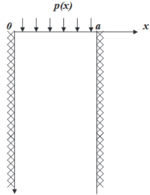
Figure 1: Geometry of the problem.

THE STATEMENT OF A PROBLEM

he elastic (G is a share module,  is a Poison’s coefficient) semi-strip, 0 x a, 0  y is considered. At the edge y0, 0 x a the semi-strip is loaded

 

y( , 0)x p x , xy( , 0) 0,x 0 x a

       (1)

where p x( ) is the known function.

At the lateral sides x0, 0  y and xa, 0  y the boundary conditions of the fixed are given

















u 0, y 0,v 0, y 0,u a y, 0,v a y, 0, 0  y (2)

(3)

3

here u x y( , )u_x



x y,



, v x y( , )u_y



x y,



are the displacements which satisfy the Lame’s equations. The Lame’s equations are written in the following form [24]

u x y u x y v x y x y

x y

v x y v x y u x y

x y

x y

2 2 2

* ₂ ₂ 0

2 2 2

* 0

2 2

( , ) ( , ) ( , )

0

( , ) ( , ) ( , )

0

 

  _ _  _

 _{ }

 

 

  

 _ _ _

 _ _ _{ }



(3)

where ₀ 1

_

_

, _* ₀ 1 1 2

  _ _    . After the expression of the constants  ₀, _* through the Muskchelishvili constant

3 4

  , one obtains the system (3) in the another form

u x y u x y v x y

x y

x y

v x y v x y u x y

x y

x y

2 2 2

2 2

2 2 2

2 2

( , ) 1 ( , ) 2 ( , )

0

1 1

( , ) 1 ( , ) 2 ( , )

0

1 1



 



 

 _   _  _

 _ _ _{ }

 

 

   

 _ _ _

 _ _ _ _ _{ }



(4)

The boundary conditions on the semi-strip’s edge are reformulated with the terms of the displacements



_{    }

_{ }

u x v x

G p x x a

x y

0

, 0 , 0

2  _   1   _  , 0 

 

  (5)









u x v x

x a

y x

, 0 , 0

0, 0

 

   

  (6)

One needs to solve the boundary value problem (2), (4)-(6) to estimate the stress state of the semi-strip.

THE GENERAL SOLVING SCHEME OF THE PROBLEMS ON THE SEMI-STRIP STRESS STATE ESTIMATION

he Fourier’s transformation is applied to the system of Lame’s equation and to the boundary conditions by the scheme









u x u x y y

dy

v x v x y y

0

( ) , cos

( ) , sin

 

_ _

   

  

   

 



  (7)

with the inverse formula









u x y

u x y

d

v x y

v x y

0

( ) cos

, 2

( ) sin ,

 

   



 _    

     

 



(8)

The initial problem has the form after this

(4)

4

u x u x v x x

v x v x u x x

u u a

v v a

2

( -1) 2 3

" ( ) ( ) ' ( ) '( )

1 1 1

( 1) 2 1

" ( ) ( ) ' ( ) ( )

1 1 1

(0) 0, ( ) 0 (0) 0, ( ) 0

             _{ }       _ _     _ _ _          _ _ _{ }  _ _ _      (9)

Here the new unknown function is inputted

  

x v x, 0 , '

  

 x v x'



, 0



. As it is seen from the boundary condition (6), u__y



x, 0



 '

 

x , so the condition (6) is satisfied automatically.

With the aim to reduce the problem to the vector boundary problem one must input the vectors and the matrixes

 

u

 

_{ }

x

y x v x       _ _    _,

_{ }

 

x f x x 3 ' 1 1 1            _      _       

, P

1 0 1 1 0 1         _            

, Q

1 0 1 1 0 1      _     _       .

Then the equations in the vector form will be written as the vector equation L y₂_

 

x  f x

 

, where L₂ is a differential operator of the second order L y₂_

 

x Iy_"

 

x 2Qy_'

 

x 2Py_

 

x , I is an identity matrix. The integral transformations also should be applied to the boundary conditions, with the aim to formulate the boundary functionals in the transformations’ domain. As a result the vector boundary problem is constructed

 

L y x f x

y y a

2

0 0, 0

       

  (10)

THE SOLVING OF THE VECTOR BOUNDARY VALUE PROBLEM

he solution of the vector boundary problem (10) will be searched as the superposition of a homogenous vector equation’s general solution y0_

 

x and a particular solution of the inhomogeneous one y1_

 

x

 

y_ x  y0_ x  y1_ x

  

These solutions were constructed with the help of the matrix differential calculation apparatus earlier [18].

 

c

 

c

 

y x Y x Y x y x

c c

1 3 1

1 2

2 4

        

   

 

where Y x i_i

 

, 0,1are the matrix system of the fundamental matrix solutions [18]:

 









 









x x

x x x x

e e

Y x Y x

x x x x

1 2

1 1 1 1

,

2 2

1 1 1 1

                          _  _   _ _   _ _            _ _    _ _   _ _     

where constants c i_i, 1, 4 are founded from the boundary conditions [18].

(5)

5

For the obtaining of the vector boundary problem’s particular solution y1_

 

x , was constructed the Green’s matrix function [18]. Elements of matrix are shown in the Appendix A.

The inhomogeneous boundary problem’s final form of the solution is constructed

 

c

 

c a





y x Y x Y x G x f d

c c

1 3

1 2

2 4 ₀

, ( )

          

   





 ₍₁₁₎

The components of (11) can be written in the next form

 

a



  

a



  

u x Y₁11 x c₁ Y₁12 x c₂ Y₂11 x c₃ Y₂12 x c₄ G11 x d G12 x d

0 0

3 1

( ) , ' ,

1 1

     __



     __



   

 

a



  

a



  

v x Y₁21 x c₁ Y₁22 x c₂ Y₂21 x c₃ Y₂22 x c₄ G21 x d G22 x d

0 0

3 1

( ) , ' ,

1 1

     __



     __



   

where Gi j,



x,



is the Green’s matrix function element in a i row and j column. The integrals with the function

 

  are calculated by the parts and the inverse integral transformations’ formulae were applied to the displacements’ transformations.





 





 





 





 

a

u x y f x y d d

v x y f x y d d

1

0 0

2

0 0

, ' , , cos

      







(12)

where f x_i



, , 

 

,g x_i , , 



,i1, 2 are known functions.

The formulae (12) would be the final ones if the unknown function  '

 

is known. For its finding one must satisfy the boundary conditions (5) which are unsatisfied yet. It should be taken into consideration that integrals in these correspondences are conditionally convergent integrals. So, before the differentiating of the displacements’ expressions, at first one must extract the weakly convergence parts at these integrals.

The substitution of (12) in the boundary conditions (5) leads to the singular integral equation

  



 

a

f x d r x x a

* * * * * *

0

' , , 0

      



here the function f



,x



contains Cauchy’s type singularities and fixed singularities on the both ends of the integration interval.

THE SOLVING OF THE SINGULAR INTEGRAL EQUATION

he changing of the variables a x x a

a a

* *

2 2

,



    is done for the passing to the integration interval



1;1



. As

a result the integral equation is transformed to the form

(6)

N. Vaysfeld et alii, Frattura ed Integrità Strutturale, 38 (2016) 1-11; DOI: 10.3221/IGF-ESIS.38.01 6

 

_{ }





















































  



 

c c x c c x

c с

c d

x x x x x x x

c x c x

d K x d r x x

x x

1 1

3,1 3,2 3,1 3,2

2 2

1 ₂ ₂ ₂ ₂

1 1

1

4 4

3 3

1

1 1 1 1

2 2 2 2 2 2

1 1 1 1

, , 1 1

2 2     _ _{ }          _ _{ } _{ }                    _        _                              _



 _   (13)

here

 

a



1



2

   _{ }  _

 

 , K x



,

  

,r x are the known regular functions, c_i,i1, 4 are shown in the Application B. The Eq. (13) is the partial case of the equation with two fixed singularities considered [21]

 







 



 















  

 

m _mk n k k

m_k k m_k k k

k

y c x y x x y

c

A x c x dy dy

i y x i _y _y _xy

K x y y dy f x m k

1 1 2 1 0 1 0 1 1 1 1

, 1 1

1

1 1 1

, , 0 Re

          _ _ _             _ _ _    





which can be rewritten as

 



  

 

A x c x c S x N x N x K x K x y y dy f x

1

0 1 1 1 1 1

1 ,              

_

 where

 





 

















m n _k k

k k _x k

k m_k k

k

x y

c

N x dy c c c x

i _y _x _y

1 2 1 ₁ 1 0 1 1 1

, 1, 1 lim ,

1 2 _

         _ _ _              





  ,

The symbol of the singular integral Eq. (13) was constructed, which has the following form, where all designations correspond to the designations in [21]

 

_

_

 

mk k k k mk k k k

c S c n R

A A

A

c S c n R

2

1 2 ,

0 ,

2

1 2 ,

0 , , , ,                                     _ _ _{  }  



(14)



1



/ ,p S_

 

z cth



i z



,

 

, ,z

 

,

             ,

 







k mk

k k k

k _k

k

n iz m

sh i z

(7)

 



































G zi i

p

G i

A z

z i z i

p p

G zi i G z i i

p p

z i i z i

p p

1

4 1 2

2 2

1 1

sinh 2 1 sinh 2 1 1

1 1

4 2 1 2 cosh 1 3

1 1

sinh 2 1 1 sinh

  _{  }              _ _  _ _         _  _  _{ }     _ _       _   _   _   _ _                _   _{ }  _   _ _             _  _  _ _ _        











G zi zi i

p p

z i i

p

1 1

16 1

1

2 1 1 sinh 1

         _   _  _            _ _   _  _  _              

here p2,   0.31 is found from the known solution of the analogical problem for an edge with the angle of openness pi/2 [25].

According to [21] one needs to find the roots of the equation A z_

 

0. The found roots of the kernel’s symbol (14) have the next form:   _1,2 0.5562 0.3690,  _3,4 1.2792 0.2380,  _5,6 3.2089 0.7127,  _7,8 5.2170 1.0251,... , where _k _k because of the problem’s statement.

The generalized method of SIE solving [22, 23] was applied for the solving of the Eq. (13). According to it the unknown function  

 

is expanded by the series in each interval

 





 





N k k k N k k k N s s 1 0 2 1

, 1; 0

, 0;1                       _  



 (15)

where

  







  







k k k k k k N k Re 2 Re 2 1

1 cos Im ln 1 ,

0, 1

2

1 sin Im ln 1 ,

                         ,

  







  







k N

k k N

k N

k k N

N k N Re 2 Re 2 1

1 cos Im ln 1 ,

, 1

2

1 sin Im ln 1 ,

                             .

The segment



1;1



is divided on 2N equal segments with the length h N

1

 . The Eq. (13) is considered when

i

h

x 1 ih ,i 0, 2N 1 2

      .

After the substitution of the unknown function (15) into the singular integral Eq. (13) one obtains system of the linear algebraic equations relatively to the unknown constants s k_k, 0, 2N1 of the expansion (15).

N

k ki i

k

s d f i N

2 1

0

, 0, 2 1





  



(16)

where d_ki,f i k_i, , 0, 2N1 are shown in the Application C.

(8)

8

THE RESULTS OF THE NUMERICAL ANALYSES

he calculations were done for the elastic semi-strip (G61.2781955 10 9 Pa,  0.33). At Fig.2 one can admit that the values of the normal stress _y _y/ ,P_x _x/P at the lateral side x0 decrease to zero with the increasing of the distance from the semi-strip’s edge. When the semi-strip’s side is a10. A similar situation is observed during the analyses of the stress   _y, _x when the semi-strip’s side is a50 (Fig.4) and a100 (Fig.6). At Fig.3 one can admit that the absolute values of the normal stress _y at the line xa/ 2, y



0;10



are higher by its absolute value then normal stress _x when the semi-strip’s side is a10. A similar situation is observed during the analyses of the stress  _y, _x when the semi-strip’s side is a50 (Fig.5) and a100 (Fig.7). As it is seen the stabilization of the stresses  _y, _x is observed when the semi-strip’s side is a50 (Fig.5) or a100 (Fig.7).

Figure 2: Normal stresses _y



0, y



,_x



0, y a



, 10. Figure 3: Normal stresses _y



a/ 2,y



,_x



a/ 2, y a



, 10.

Figure 4: Normal stresses y



0, y



,x



0, y a



, 50. Figure 5: Normal stresses y



a/ 2,y



,x



a/ 2, y a



, 50.

(9)

9 Figure 6: Normal stresses y



0, y



,x



0, y a



, 100. Figure 7: Normal stresses y



a/ 2,y



,x



a/ 2, y a



, 100.

CONCLUSIONS

1. The proposed solving method reduced the initial problem to the singular integral equation, which has the two fixed singularities at the end of the integration’s interval. The special generalized scheme of SIE solving was applied with the aim to take these singularities into consideration.

2. The proposed approach may be applied to the solving of the elasticity mixed problem for the semi-strip with a crack. 3. The analyses of the numerical results show that the taking into consideration the existence of the two fixed singularities of the solution gives the possibility to obtain the numerical result on the distance less than a/1000 to the angular point of the semi-strip in comparison with the usual approach to the solving, allowing to get the stable results only on the distance to the angular points not less than a/10.

APPENDIX A









_{ }





_



 









 















 







 









ch a x ch a x

G x

sh a

sh a sh a x xsh a x

sh a

ash a x a x ash a x ach a ch a x ch a x

11

2

,

2 1

1

2 1

     



  

     

 

         

    

 





 _      





              _





_{ }

_

 













































ach a

G x sh a x

sh a _{ch a}

x sh a x ch a x a x x ch a x a x

12 ₂

1 ,

2 1 ₁ ₁

sgn sgn



  

  _ _

         

 

 _   

 _ _





(10)





 





_

_{ }

_

 



_

_

































ach a

G x sh a x

sh a _{ch a}

x sh a x ch a x a x x ch a x a x

21 ₂

1 ,

2 1 ₁ ₁

sgn sgn       _ _              _     _ _                  _









_{ }





 









 

















 











 









ch a x ch a x

G x

sh a

sh a ch a x ch a x

sh a

a x sh a x a x sh a x a ch a ch a x ch a x

22 2 , 2 1 2 1                                       _                         _

APPENDIX B

























































G G G G

c c c c c

G G G G G

c c c c c

0 1 2 2 3,1

3,2 3,1 3,2 4 4

2 3 1 2 2 2 2 4 2

0, , , , ,

2 1 1 2 1 2 1 2 1 1

4 2 1 4 2 4 2 1 16 16

, , , ,

2 1 1 2 1 1 2 1 1 1 1

                                                                                               

APPENDIX C

 





























































 

i i ki k

i i i _i _i _i _i

i i

i

i i

ki k

i i

c c x c c x

c c с

d

x x x _x _x _x _x

c x c x

K x d k N i N

x x

c c с

d

x x

0

3,1 3,2 3,1 3,2

1 2 2

2 2 2 2

1

4 4

3 3

1 2 2

1 1 1 1

2 2 ₂ ₂ ₂ ₂

1 1 1 1

, , 0, 1, 0, 2 1

2 2 2        _ _ _ _   _ _                         _{ }            _{ } _{ } _{ } _{ }                    _      































































 

i i

i _i _i _i _i

i i

i

i i

c c x c c x

x _x _x _x _x

c x c x

K x d k N i N

x x

f r x i N

1

3,1 3,2 3,1 3,2

2 2 2 2

0

4 4

3 3

1 1 1 1

2 ₂ ₂ ₂ ₂

1 1 1 1

, , 0, 1, 0, 2 1

2 2

, 0, 2 1

   _ _ _ _   _ _                     _ _                            _   



 REFERENCES

[1] Vorovich, I. I., Kopasenko, V. V., Some problems of elasticity theory for the semi-strip. (in Russian), Prikladnaya matematica i mekchanica, 30(1) (1966) 128-136.

[2] Pickett, G., Jyengar, K. T. S., Stress concentrations in post-tensioned prestressed concrete beams, J. Technol., India, 1(2) (1956).

(11)

11 [4] Koiter, W., Alblas, J., On the bending of cantilever rectangular Plates, Proc. Koninke Nederl. Acad. wet. B., 57(2)

(1954).

[5] Aglovyan, L. A., Gevorkyan, R. S., About some mixed problems of elasticity theory for the semi-strip (in Russian), News of academy of science Armenian SSR, Mechanics, 23(3) (1970) 3-13.

[6] Trapeznikov, L. P., Influence lines for the normal tensions in semi-strip (in Russian), News of USSR n.-i. of the hydromechanical institute, 73 (1963).

[7] Kolchin, G. B., Plyat, Sh. N., Sheykner, N. Ya., Some problems of the themoelasticity for the rectangular areas (in Russian), Shtiica, (1980).

[8] Suchevan, V. G., The tensioned state of the elastic semi-strip with fixed edges (in Russian), Matematiceskie issledovaniya, 40 (1976) 122-135.

[9] Thecaris, P. The stress distribution in a semi-infinite strip subjected to a concentrated load, Trans. J. Appl. Mech., 26(3) (1959) 401–406.

[10]Johnson, M. W., Little, R. W., The semi-infinite elastic strip, Q. Appl. Math., 22(4) (1965) 335-344. [11]Horvay, G., The end problem of rectangular strips, J. Appl. Mech., 20 (1953) 87-94.

[12]Horvay, G., Born, J., Some mixed boundary-value problems of the semi-infinite strip, Journal of Applied Mechanics, 24(2) (1957) 261-268.

[13]Benthem, J.P., A Laplace transform method for the solution of semi-infinite and finite strip problems in stress analiesis, Quart. J. Mech. and Appl. Math., 16(4) (1963) 413-429.

[14]Gogoleva, O. S., The examples of solutions of the first main boundary problem of elasticity theory in the semi-strip (symmetrical problem) (in Russian), Journal Omskiy gosudarstvenniy universitet, 145(9) (2012) 138-142.

[15]Kovalenko, M. D., Shulyakovskaya, T. D., Expansion of Fadle-Papkovich functions in the strip. Bases of theory (in Russian), Mechanica tverdogo tela, 5 (2011) 78-98.

[16]Menshova, I. V., Lapikova, E. S., The semi-strip with lateral edges rigidity, working for tension-compression (in Russian), Journal ChGPU named I. Ya. Yakovlev, series: Mechanic of the limited state, 20(2) (2014) 106-118.

[17]Popov, G. Ya., About new transformations of the elasticity resolving equations and the new integral transformations with their application to the boundary problems of mechanics, Intern Appl. Mech., 39 (2003) 1046-1071.

[18]Vaysfel’d, N. D., Zhuravlova, Z. Yu., On one new approach to the solving of an elasticity mixed problem for the semi-strip, Acta Mechanica, 226(12) (2015) 4159-4172, DOI: 10.1007/s00707-015-1452-x.

[19]Ciavarella, M., Paggi, M., Carpinteri, A., One, no one, and one hundred thousand crack propagation laws: a generalized Barenblatt and Botvina dimensional analysis approach to fatigue crack growth, Journal of the Mechanics and Physics of Solids, 56(12) (2008) 3416-3432.

[20]Carpinteri, A., Paggi, M., Analytical study of the singularities arising at multi-material interfaces in 2D linear elastic problems, Engineering fracture mechanics, 74(1) (2007) 59-74.

[21]Duduchava, R. V., Integral convolution equations with discontinuous presymbols, singular integral equations with fixed singularity and their application to the mechanical problems (in Russian), Tbilisi, Mecniereba, (1979).

[22]Kryvyy, O. F., Tunnel Internal Crack in a Piecewise Homogeneous Anisotropic Space, Journ. of Mathematical Sciences, 198(1) (2014) 62-74.

[23]Kryvyi, O. F., Mutual influence of an interface tunnel crack and an interface tunnel inclusion in a piecewise homogeneous anisotropic space,Journ. of Mathematical Sciences, 208(4) (2015) 409-416.

[24]Popov, G.Ya., The elastic stress' concentration around dies, cuts, thin inclusions and reinforcements (in Russian), Nauka, Moskow (1982).