Evolution – Equivalent Length and Cumulative Mutation
Density
Hong-Da Chen1,2, Wen-Lang Fan2,3, Sing-Guan Kong1,2, Hoong-Chien Lee1,2,4,5*
1Graduate Institute of Systems Biology and Bioinformatics, National Central University, Chungli, Taiwan,2Department of Physics, National Central University, Chungli, Taiwan,3Genomic Research Center, Academia Sinaca, Taipei, Taiwan,4Cathay Medical Research Institute, Cathay General Hospital, Taipei, Taiwan,5National Center for Theoretical Science, Shinchu, Taiwan
Abstract
Background:Segmental duplication is widely held to be an important mode of genome growth and evolution. Yet how this would affect the global structure of genomes has been little discussed.
Methods/Principal Findings: Here, we show that equivalent length, or Le, a quantity determined by the variance of
fluctuating part of the distribution of thek-mer frequencies in a genome, characterizes the latter’s global structure. We computed theLes of 865 complete chromosomes and found that they have nearly universal but (k-dependent) values. The
differences among theLeof a chromosome and those of its coding and non-coding parts were found to be slight.
Conclusions:We verified that these non-trivial results are natural consequences of a genome growth model characterized by random segmental duplication and random point mutation, but not of any model whose dominant growth mechanism is not segmental duplication. Our study also indicates that genomes have a nearly universal cumulative ‘‘point’’ mutation density of about 0.73 mutations per site that is compatible with the relatively low mutation rates of (1*5)|10{3/site/Mya
previously determined by sequence comparison for the human andE. coligenomes.
Citation:Chen H-D, Fan W-L, Kong S-G, Lee H-C (2010) Universal Global Imprints of Genome Growth and Evolution – Equivalent Length and Cumulative Mutation Density. PLoS ONE 5(4): e9844. doi:10.1371/journal.pone.0009844
Editor:Josh Bongard, University of Vermont, United States of America
ReceivedNovember 4, 2009;AcceptedFebruary 8, 2010;PublishedApril 14, 2010
Copyright:ß2010 Chen et al. This is an open-access article distributed under the terms of the Creative Commons Attribution License, which permits unrestricted use, distribution, and reproduction in any medium, provided the original author and source are credited.
Funding:This work was funded by the National Science Council (ROC) (http://web1.nsc.gov.tw/mp.aspx?mp=7), Cathay General Hospital (http://www.cgh.org. tw/en/index.html), National Central University (http://www.ncu.edu.tw/e_web/index.php). The funders had no role in study design, data collection and analysis, decision to publish, or preparation of the manuscript.
Competing Interests:The authors have declared that no competing interests exist.
* E-mail: [email protected]
Introduction
Evolution has many facets, and one that is particularly accessible to quantitative analysis is the evolution of genomic sequences. In particular, the study of point mutations (here used in the sense that includes relatively small insertions and deletions, or indels) on genes has led to deep understandings of many aspects of genome evolution [1,2]. Point mutation however cannot be the main force driving genome growth, because it does not give rise to gene duplication [3–8], and because the pace of evolution based on point mutation alone would be too slow. Gene duplication is a product of segmental duplication (SD). In fact, genomes are replete with vestiges of duplication [9–11], not only in the form of homologous genes, but also as transposons [12–14], pseudogenes [15–18], and many other types of coding and non-coding repeats [19–22]. There is also evidence of large-scale genomic rearrange-ments [23–27] and whole genome duplications [3,28–30]. This has led to the generally held view that SD is an important mode of genome growth and evolution.
If products of SD are so prevalent in genomes, we expect the SD’s in a genome, collectively, to leave a large imprint on the global structure of its host, one that is detectable using means not relying on sequence alignment, which in any case is not suitable
for global studies. One may reasonably expect a study to understand the formation of such an imprint to yield useful insights into the global pattern of genome growth and evolution, yet no such effort has been made.
characteristics of genomic FFDs sharply distinguishes them from their random counterparts under all circumstances.
In this study we used the FFD to define the equivalent lengths (Le’s; one for eachk) of a sequence and discovered a universality in these quantities. We then identify these Le’s and their small values, as a clear and distinct global imprints of genome growth and evolution. (TheLeof a sequence is inversely proportional to the FFD part of the variance and is defined such that theLeof a random sequence is its own true length. Therefore, a sequence whose equivalent length isLe has the characteristic randomness of a random sequence of length Le.) We computed the Le of about 900 complete chromosomes, all the complete sequences at the time of download from GenBank, fork= 2 to 10, and found some unexpected and useful results: Roughly, the complete set of about 7400 k-dependent whole-chromosome Le’s is well represented by the universal formulaLfucg
e (k) =Le2ea0(k{2)where Le2*310z{290150 b (base pair) and a0= 0.92. The formula means that, for the smallerk’s, the universal genomicLeis only a small fraction of the genome length even for the shortest genomes. Another unexpected result is the small difference between the Le’s of coding and non-coding parts. In our successful attempt to describe these results in a simple genome growth model driven by random segmental duplication, we obtained a universal cumula-tive point mutation density of r= 0.73+0.07/site for genomes. This value is compatible with the relatively low mutation rates previously determined by sequence comparison for the human andE. coligenomes [37–39].
Results
Only FFD contains non-trivial information
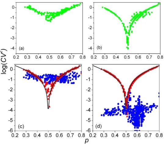
A key to our approach to the analysis of genomic sequences is the decomposition ofCV2–CV is the coefficient of variation of an FD – into FFD and NFFD components (Methods). This is illustrated in Fig. 1, which shows the values ofCV2for 2-mers; results for other k’s are similar. The full CV2 of genomic sequences (Fig. 1(a)) differs from that of their matching random sequences (Fig. 1(b)) clearly only whenDp{0:5D 0.1, wherepis the fractional A/T-content. (A genome and its matching random sequence have the same length and base composition.) The situation becomes much clearer whenCV2is decomposed into its FFD and NFFD parts,CVnf2andCVfl2, respectively. While the values of CVnf2 for the two type of sequences are almost indistinguishable ((red) triangles, Fig. 1(c,d); the two ‘‘volcano’’ curves are identical, being both given by the theoretical prediction, Eq. (12)), the values ofCVfl2for genomes and random sequences are drastically different ((blue) bullets, Fig. 1(c,d)). The genomic CVfl2 span a narrow band ranging from 0.01 to 0.1, while the randomCVfl2are several orders of magnitude smaller. In fact for random sequences the value ofCVfl2 is well understood to be inversely proportional to sequence length (Eq. (13), and below). Clearly, if random sequences are used as controls to discuss the non-random properties of genomic sequences when the distinction between FFD and NFFD is not made, then it is possible that conflicting conclusions [32,40–43] may be drawn.
Figure 1. Fluctuating and non-fluctuating parts of variance.(a) Variances of 2-mer frequency distribution of 865 complete sequences. (b) Same as (a) but for for 865 matching random sequences. Bottom: same data as in top plots, but with each variance split into non-fluctuating (triangles) and fluctuating (bullets) parts, for (c) genomes and (d) matching random sequences. The ‘‘volcanic’’ curves through the non-fluctuating data in (c) and (d) plot theoretical values given by Eq. (12).
doi:10.1371/journal.pone.0009844.g001
Genomicleis approximately a constant of sequence length
Throughout this paper we use le to denote generically the equivalent length of any sequence (Eq. (14), Methods), and reserve Lefor denoting entire sequences such as a complete chromosomes. Fig. 2 showsle versus segment lengthlsfor segments taken from the chromosomes of four model organisms:E. coliK12;C. elegans, Chr. (chromosome) 1; A. thaliana, Chr. 1;H. sapiens, Chr. 1, and matching random sequences. The computation is carried out only when ls is at least four times 4k, since for shorter lengths the systematic error becomes too large. It is seen that whereas theleof random sequences closely tracksls, as expected, theleof genomic sequences quickly levels off to a saturation value Le(k). These results forls 5 kb may be summarized in terms of the scaling relationle!(ls)c. Then we have the two distinct classes c&1 for random sequences andc&0 for genomic sequences. This scaling relation is not the same as the long-range correlation and scale-invariance observed in binary analyses of long genomic sequences [44–46]. In Fig. 2Leis seen not to depend strongly on organism. For smallk,Le(k)is diminutive relative to genome length:*0.35 and*1.0 kb whenk= 2 and 4, respectively, growing to 600 kb when k= 10. Within a genome, the apparent invariance of CV (not CVfl) with respect to segment length was noted in [47–49] and the relation between Shannon information and a quantity similar toCVfl was discussed in [50].
Whole chromosomes have nearly universalLe(k)
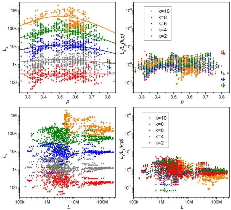
A list of the 865 complete chromosomes studied here is given in Table S1, and a list ofLe(k)’s,k= 2 to 10, for the chromosomes is give in Table S2. Fig. 3 showsLe(k), as a function ofp(top panels) and chromosome length L (bottom panels), computed from the complete chromosomes for evenk’s up tok= 10. Table 1 gives the Le(k),k= 2 to 10, of chromosomes of seven model organisms. It is seen that Le(k) has a clear dependence on k, is essentially independent of sequence length, and has a weak dependence onp. Fig. 4 gives Le(k) for odd k’s averaged over categories of
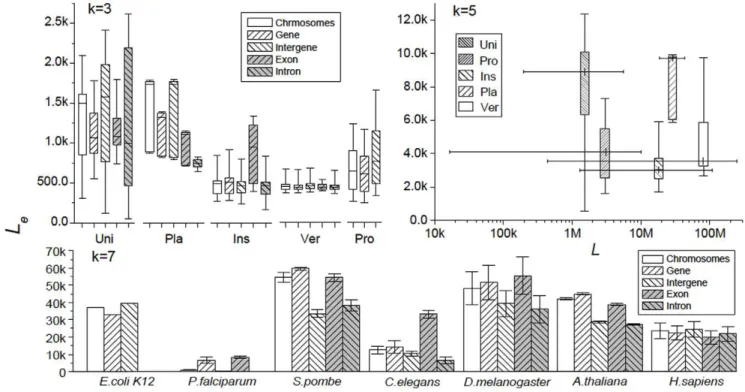
organisms and over chromosomes in model organisms (for more detailed results see Table S3). The k= 5 data reconfirms the absence inLeof a systematic dependence on chromosome length (similarly for otherk’s). In thek= 3 and 7 plots Le’s are given separately for the whole chromosome, and genic (gn), and inter-genic (ig), exon (ex) and intron (in, when applicable) concatenates (Methods). The unicellulars are seen to have the largest variation inLe, especially for theigandinregions. This partly reflects the fact that this category includes two phylogenetically remote groups, protists and fungi. In contrast, the relatively small variation in the vertebrateLe reflects the fact that, compared to organisms in other categories, vertebrates are phylogenetically very close. Two examples in opposite extremes are shown in the bottom panel of Fig. 4 (k= 7): the malaria causing parasite P. falciparumwith especially smallLe’s, and the fungusS. pombewith relatively largeLe’s. This indicates that the chromosomes of P.
falciparum and S. pombe are much less and much more random,
respectively, than the genomic norm. Although such inter-category, inter-species and inter-regional differences are signifi-cant, they pale when compared with the difference betweenLe and true chromosome lengths. Table 2 listsLe(k),k= 2, 5, 7 and 10, averaged over all 865 sequences, for whole chromosome and the four types of concatenates.
Summary of genomic data
We summarize the trends of genomic data: (a)Le(k)increases withk. (b) For givenk,Lehas no systematic dependence onLand has a weak dependence onp. (c) For given k, Le for different organisms are of the same order of magnitude. (d) Within a genome, Le differs little among chromosomes. (e) There is remarkable agreement between thegnandexdata sets. (f) There is not a significant difference between theLe(k)’s for coding (ex and gn) and non-coding (in and ig) regions, and the agreement between the two regions improves when that fact that coding regions tend to be GC-rich is taken into account (Text S1 and Fig.
Figure 2. Segmental equivalent lengths from four model organisms.Equivalent lengthleversus sequence lengthlsfor genomic (hollow
symbols) and matching random (solid symbols) sequences. Genomic segments are fromE. coli(p), worm (C. elegans(chromosome)I,D), mustard (A. thaliana I,+), and human (H. sapiens I,œ). Eachlein the form of mean+SD is averaged over the maximum number of non-overlapping segments (of
lengthls) in the chromosome or, if the chromosome is longer than 20ls, 20 randomly selected segments.
S1). We remark that in splicing the gn concatenate genes in positive and negative orientations from asinglestrand of DNA are concatenated, without inverting the negatively oriented genes (Methods). Similarly for theexconcatenate.
Discussion
Universal Le is not a result of inter-chromome similarity ink-mer-content
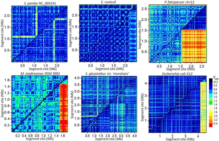
Fig. 5 shows intra-chromosome k-mer-content similarity plots (Methods) for six representative chromosomes. In the plots, a small value ofgsim ( 0.2, black-blue) indicates high degree of similarity, and a large value ( 1, cyan to red) indicates the opposite. A general trend is that local k-mer-content within a chromosome is fairly homogeneous [51,52] on a scale as small as 50 kb. When
k-mer-contents of coding and non-coding parts show a significant difference, as is seen in the case ofP. falciparum,M. stadtmanae, andE. coli, it is mainly caused by thegnpart being substantially richer in GC content than theigpart (Table 3). Nevertheless, becauseLeis defined such that first-order dependence in base composition is removed, within a chromosome the Le’s for the gn and ig parts and for the whole chromosome generally have similar values (Table S3,SI).
Fig. 6 compares the intra-E. coli plot with inter-chromosome plots ofE. coli versus seven other organisms whose phylogenetic distances toE. colirange from close to remote. The approximate monochromaticity of each plot reconfirms our previous observa-tion thatk-mer-content within a chromosome has a high degree of homogeneity (on a scale of 100 kb). We see close correlation between phyogenetic distance and the shades (colors) of the seven inter-chromosome plots. Fig. 7 gives the meangsim for the plots
Figure 3. Chromosomal equivalent length (Le) versuspandL.Top panels:Leversusp; bottom panels:LeversusL. Each piece of data gives theLe
from a complete chromosome:+(red),k= 2;p(gray),k= 4;D(blue),k= 6,œ(green),k= 8,1(orange),k= 10. Lines in top-left panel represent the ‘‘universality class’’Lfucg
e (k;p) (Eq. (1)). The right panels show the collapse of genomic data to around unity when the genomicLe(k)is divided byLfeucg(k;p).
doi:10.1371/journal.pone.0009844.g003
and P-values from Student t-tests for the null assumption that the inter-chromosome plots are the same as the intra- E. coli plot. These results verify that the observed near universal value in Le is not cause by similarity in k-mer-content among chromosomes.
As an aside, we note that in Fig. 6 the plot forS. pombeindicates a*100 kbigsegment around the 1.1 Mb site has extraordinary low similarity with respect to all other regions of the chromosome. This could be the result of a non-genic horizontal/lateral transfer [53,54] and suggests that similarity plots may be useful for locating such events.
A universal formula forLe
The 7360 pieces of data in the ‘‘All’’ set in Table 2 is well represented by the empirical formula,
Lfucg
e (k;p)~Le2exp ((k{2)a(p));(2ƒkƒ10) ð1Þ
a pð Þ~ a0
1z tanhp2zð1{pÞ2{0:5pi ð2Þ
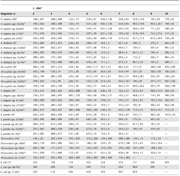
Table 1.Genomic equivalent lengths for model organisms.
Le(kb)d
Organism\\\k 2 3 4 5 6 7 8 9 10
H. sapiens(24)a .188+.021 .448+.046 1.22+.13 3.39+.41 9.34+1.36 23.8+4.4 53.9+12.6 103+29 170+54
H. sapiens(gn; 43.2%)b .185+.022 .440+.048 1.20+.14 3.31+.42 9.02+1.33 22.4+4.0 49.2+10.9 90.5+23.7 144+42
H. sapiens(ig; 63.6%)b .190+.021 .452+.045 1.24+.13 3.44+.41 9.51+1.36 24.5+4.5 56.6+13.4 111+32 186+61
H. sapiens(ex; 2.1%)b,c .171+.019 .412+.042 1.12+.12 3.07+.39 8.21+1.26 19.9+3.8 41.9+10.3 72.2+21.6 117+22
H. sapiens(in; 37%)b,c .182+.020 .434+.043 1.18+.13 3.26+.40 8.84+1.34 21.9+4.2 47.7+11.5 87.2+24.9 139+45
A. thaliana(5)a .373+.005 .871+.013 2.20+.04 5.89+.10 16.0+.3 42.1+.8 109+2 273+7 642+20
A. thaliana(gn; 55.8%)b .333+.004 .822+.011 2.06+.03 5.57+.08 15.9+.2 44.9+.7 129+2 367+6 981+22
A. thaliana(ig; 44.1%)b .394+.007 .798+.014 1.94+.04 4.95+.10 12.3+.2 28.9+.6 66.1+1.5 144+4 296+12
A. thaliana(ex; 32.9%)b,c .288+.003 .715+.007 1.75+.02 4.72+.05 13.6+.1 38.9+.4 113+2 326+7 865+35
A. thaliana(in; 16.1%)b,c .350+.003 .752+.006 1.80+.02 4.42+.04 11.1+.1 27.3+.4 68.1+1.0 167+3 400+1
Drosophila(4)a .409+.142 .957+.213 2.54+.46 6.90+1.17 18.7+3.2 48.2+9.5 117+31 268+102 676+294
Drosophila(gn; 56.4%)b .432+.108 1.02+.15 2.71+.30 7.35+.85 20.0+2.8 51.6+9.9 127+35 326+120 756+321
Drosophila(ig; 43.5%)b .392+.194 .882+.305 2.30+.66 6.15+1.57 16.1+3.3 39.4+7.5 90.0+28.1 235+87 536+231
Drosophila(ex; 23.9%)b,c .478+.023 1.16+.09 2.82+.41 7.55+1.39 21.0+4.2 55.6+10.7 140+29 377+111 907+324
Drosophila(in; 34.8%)b,c .378+.145 .833+.168 2.15+.30 5.65+.73 14.8+2.3 36.2+7.9 84.0+26.2 207+79 458+198
C. elegans(6)a .119+.012 .258+.032 .624+.089 1.63+.26 4.46+.78 12.6+2.3 35.5+6.9 98.8+21.0 264+63
C. elegans(gn; 58.6%)b .126+.017 .284+.047 .697+.135 1.83+.40 5.06+1.21 14.3+3.7 40.8+11.1 114+34 306+99
C. elegans(ig; 41.3%)b .109+.009 .226+.022 .539+.061 1.39+.18 3.78+.51 10.5+1.5 29.3+4.5 79.5+13.6 202+41
C. elegans(ex; 27.5%)b,c .184+.010 .483+.025 1.28+.07 3.64+.23 10.9+.7 33.2+2.4 102+8 306+25 822+58
C. elegans(in; 32.3%)b,c .085+.015 .169+.037 .382+.096 .939+.265 2.44+.73 6.52+1.99 17.4+5.3 45.4+14.1 113+37
S. pombe(3)a .362+.010 .894+.030 2.41+.09 6.74+.28 19.2+.9 54.6+3.0 153+11 402+39 1013+39
S. pombe(gn; 57.8%)b .339+.002 .880+.006 2.38+.01 6.82+.05 20.2+.2 59.6+.8 173+6 455+42 —
S. pombe(ig; 42.1%)b .364+.019 .812+.045 2.08+.12 5.31+.32 13.5+.8 33.6+2.1 81.7+5.8 187+16 —
S. pombe(ex; 53.9%)b,c .357+.007 .889+.018 2.40+.06 6.73+.18 19.2+.6 54.4+2.3 149+10 374+42 —
S. pombe(in; 3%)b,c .361+.007 .898+.017 2.41+.06 6.53+.14 17.0+.4 38.2+3.1 — — —
Plasmodium(14)a 1.40+.20 .287+.019 .376+.023 .512+.036 .729+.059 .998+.089 1.34+.13 1.73+.19 —
Plasmodium(gn; 56%)b .595+.118 .659+.085 1.02+.12 1.86+.29 3.59+.74 6.73+1.86 12.3+4.3 16.3+10.4 —
Plasmodium(ig; 44%)b .665+.108 .111+.017 .130+.017 .162+.022 .212+.031 .276+.042 .357+.057 .398+.032 —
Plasmodium(ex; 53%)b,c .515+.058 .717+.060 1.12+.07 2.10+.11 4.21+.23 8.30+.56 16.0+1.3 32.0+1.6 —
Plasmodium(in; 5.7%)b,c .163+.019 .052+.002 .064+.003 .076+.003 .095+.004 .116+.003 — — —
E. coli(1)a .373 .729 1.74 4.52 12.6 37.0 111 328 879
E. coli(gn; 88.7%)b .346 .656 1.56 4.05 11.3 33.0 98.9 292 —
E. coli(ig; 11.2%)b .553 1.22 2.60 6.33 16.0 39.3 83.9 — —
Le(k),k= 2 to 10, of chromosomes of model organisms. TheLe’s given are mean+SD averaged over chromosomes of the organism, except for the single chromosome E. coli.See Table S2 for list of all computedLe(k)’s. (a) Number in parentheses indicates total number of complete chromosomes in organism. (b) Abbreviations:gn,
gene;gn, intergenic;ex, exon;in, intron. Percentage given indicates portion of complete sequence. ‘‘N-runs’’ or gaps in sequences are not counted. (c)Exandin
segments selected as given by Genbank; sum of percentages forexandinmay be less than or exceed that ofgndue to incomplete or duplicated segments. (d)Le(k)
wherea0= 0.92,Le2~310z{290150b, and = 0.50+0.05. The central values of the formula are shown as solid lines in Fig. 3 and listed as the entries in the row labeledLfucg
e in Table 2. The denominator in Eq. (2) represents the residualp-dependence indicated in the data in Fig. 3; it works well even for chromosomes with large Dp{0.5D
(Table S4, SI). For the vast majority of genomic Le’s,
x2:ln2(L
e(k)/Lfeucg(k;p))(Text S1) is less than 1 (Fig. S2) and, averaged over the 7360 pieces of data in the ‘‘All’’ set,Sx2T= 0.43. This means that on average the genomicLeis within a factor of two
ofLfucg
e (k;p). In recognizing that genomes as a category exhibit such a non-trivial common feature which is itself the manifest of an underlying but yet undetermined cause, we say genomes belong to a universality class. It is realized that Eq. (1) cannot be extended tok much greater than 10 (and not even to 10 for some of the smaller chromosomes), because a meaningful value for Le(k) may be extracted only when a sequence is at least4kz1bases long.
A universal formula for the standard deviation from the fluctuating part ink-mer frequency
The short genomicLe(relative to actual chromosome length) is a direct consequence of the genomicCVflbeing much larger than its random-sequence counterpart. If we approximatea(p)in Eq. (1) by a0 and approximate the factorbk in Eq. (14) (Methods) by unity, then through Eq. (14) we convert Eq. (1) to a universal formula for them-set-averaged standard deviation for thek-mer FFD:
s
sfl(k)&0:14{z00::050410
{k=2L, ð3Þ
where L is the sequence length. The formula is meant to be applicable so long as L is several times greater than 4k. For sequences withp&0.5,ss2
flreduces to the usual variance. Note that for random sequencessfl(k)*L1=24{k=2. SinceLis large, genomic
s
sflcan be orders of magnitude greater than its random counterpart. For instance, for the 4.6 Mb chromosome, thek= 4 values forssfl given by Eq. (3), the actual chromosome (m-averaged), and a random sequence are 6440 b, 6230 b, and 134 b, respectively, and for the 228 Mb human chromosome 1, the corresponding values are 319,000 b, 380,000 b, and 943 b, respectively. To give statistical meaning to such differences, Table 4 examines universal genomes of
Figure 4. Averaged equivalent lengths for complete chromosomes and concatenates.The concatenates are: ‘‘gene’’ (gnin main text), coding regions; ‘‘intergene’’ (ig), non-coding or intergenic regions; ‘‘exon’’ (ex), exons ingn(for eukaryotes); ‘‘intron’’ (in), introns ingn. Top left,Le
(k= 3) averaged over phylogenetic categories (Uni, unicellulars; Pla, plants; Ins, insects; Ver, vertebrayes; Pro, prokaryotes); top right,Le(k= 5) versus
chromosome length average over categories; bottom,Le(k= 7) for seven model organisms averaged over chromosomes. Boxes indicate data in the
10, 25, 50, 75 and 90% range. doi:10.1371/journal.pone.0009844.g004
Table 2.Average genomic equivalent lengths.
Le(kb)
Category (k= ) 2 5 7 10
All :359z:333 {:172 4:56
z3:60 {2:01 33:7
z30:0 {15:9 388
z524 {223 gn(41.8%) :317z:253
{:141 4:21 z2:82 {1:67 31:2
z23:7 {13:4 337
z396 {186 ig(59.6%) :462z:879
{:302 4:99 z4:49 {2:36 31:6
z26:9 {14:5 213
z170 {95 ex(3.3%) :292z:215
{:122 4:40 z2:55 {1:62 35:3
z20:8 {13:1 620
z298 {201 in(31.8%) :348z:679
{:230 3:65 z2:55 {1:50 23:5
z13:9 {8:7 213
z206 {105 Lfucg
e (p= 0.5) :310
z:290 {:150 4:90
z4:58 {2:24 30:1
z28:1 {13:8 487
z455 {235 RSD model :597z:756
{:351 4:79 z0:82 {0:70 32:0
z7:0
{5:8 510 z211 {149
Le(k),k= 2, 5, 7 and 10, averaged over 865 chromosomes. Total sequences
length is about 2.2|1010bases. Abbreviations: All, complete chromosome;gn, genes;ig, intergenic;ex, exons;in, introns. Percentage given indicates portion of complete sequence.Lfucg
e is defined in Eq. (1) and RSD results are averaged over
200 model sequences. See Table S4 forLe(k)of otherkvalues.
doi:10.1371/journal.pone.0009844.t002
various lengths and gives the fractions of 2-mers and 9-mers (in the genomes) whose frequencies have P-values that are less than Pn– the P-value corresponding to n standard deviations away from the expected frequency in a random sequence – forn= 3, 6, and 8, respectively. Because ssfl(k)=s
frang
fl (k)!L1
=2(0:4)k=2, the fraction
increases with decreasingkand increasingL(for a given n). For instance, for a sequence 4.6 Mb long (length ofE. colichromosome), fourteen of the sixteen 2-mers have P P8( = 1.3|10{15), whereas only 26,000 of the 262,144 9-mers are so. In comparison, for a
sequence 226 Mb long (length of human chromosome 1), all sixteen 2-mers and 213,000 of the 9-mers are so.
Segmental duplication shortensle
We now discuss probable causes for the formation of the universality class. We first list some general properties of the ratio rofleto the sequence lengthl: if the sequence is (nearly) random thenr( =le/l)&1; if it is far less random than a random sequence of lengthlthenr%1; if it is essentially ordered thenr&0; if it is
Figure 5. Intra-chromosomes similarity plots.Plots are fork= 2 (Methods). Sliding window has width 25 kb and slide 10 kb; pixel size is 10 kb by 10 kb. In each plot, the coordinates for the upper-left triangle are sites along the chromosome (chr), and those for the lower-right triangle are along a concatenate composed of gene (gn, left side) and intergene (ig, right side) parts. In effect, the upper-left triangle showschr-chrsimilarity, and the lower-right triangle showsgn-gn(lower-left sub-triangle),ig-ig(upper-right sub-triangle), andgn-ig(rectangular) similarities in three separate regions. The lengths of thegnandigparts are given in Table 3.
doi:10.1371/journal.pone.0009844.g005
Table 3.Intra-chromosome similarity indexes.
Length (Mb)/p Averagegsim
Organism chr gn ig chr-chr gn-gn ig-ig gn-ig
S. pombeChr. 1 2.45/0.64 1.40/0.61 1.05/0.69 0.648 0.569 0.615 0.647
E. cuniculi(genome) 2.50/0.53 2.15/0.53 0.35/0.55 0.527 0.481 0.450 0.666
P. falciparumChr. 13 2.73/0.82 1.55/0.79 1.18/0.87 0.801 0.742 0.641 2.11
M. stadtmanae 1.77/0.73 1.51/0.71 0.26/0.83 0.805 0.782 0.757 2.52
S. glossinidius morsitans 4.17/0.46 2.15/0.44 2.02/0.47 0.638 0.510 0.635 0.729
E. coli K12 4.64/0.50 4.12/0.49 0.52/0.58 0.517 0.481 0.548 1.63
the n-fold replication of a random sequence, then r&1/n. We illustrate how segmental duplication can cause a sequence to have rmuch less then one, by considering the effect of a generalization of the operation of replication onle. To be specific we label XY a concatenate composed of X and Y. If Y is a coarse-grained rearrangementof X, then, provided the scale of the rearrangements is not too small,le(X)&le(Y) and concatenating X and Y is similar to doubling X by replication, hence le(XY) will be nearly equal to le(X).
In general, if thek-mer-contents of X and Y are similar, then (provided the sequences are sufficiently long) we expect
le(XY)&le(X)&le(Y). Conversely, if thek-mer-contents of X and Y are significantly different, then we expect le(XY)wmin(le(X), le(Y)) (see Text S1 for an expanded discussion, including formulas given in Table S5). Results for testing these simple rules with real sequences are shown in Table 5. We expect agreement with theory to improve with increasing sequence length (l). The first two rows of results in Table 5 verify that for random sequenceris always close to one, or le&l. The results for AA0 and BB0 show that concatenating two equal-length segments from thesame chromo-some is indeed like doubling a sequence by replication. Chromosomes labeled Ci have k-mer-contents relatively more similar to A (Figs. 4 and 5), thereforele(ACi)&le(AA0)&le(A) as expected. Chromosomes labeled Di and B have k-mer-contents more dissimilar to A, thereforele(AX)wmin(le(A),le(X)). The case of AD4, where D4isH. sapiens chr. 1, is not an exception to the rule even fork= 2, because le(D4)<le(A). In the bottom portion of Table 5 the approximate relationle&n2le0 (Table S5;le0 is the equivalent length of the genomic portion andnis the ratio of the
Figure 6. Intra-E. coliand inter-chromosome similarity plots.The plots are those ofE. colichromosomevs:the chromosomes of, left to right and top to bottom,E. coli, E. coli UT189, Salmonella, the delta-proteobacteria S. aciditrophicus, the cyanobacteriaSynechocystis, the archaea P. aerophilum, chromosome 5 of the fungusA. fumigatus, and the first 4.5 Mb segment from chromosome 1 ofH. sapiens. Coordinates are sites along the sequence. Sliding window width is 100 kb and slide is 25 kb, pixel size is 25 kb by 25 kb.
doi:10.1371/journal.pone.0009844.g006
Figure 7. Comparison of inter-chromosome similarity matrices.
Mean values and SD of the eightgsim-plots (ofgsim-matrices) shown in
Fig. 6 and P-values for the null assumption that the 2nd to 7th cases are the same as the 1st case.
doi:10.1371/journal.pone.0009844.g007
Table 4.P-values fork-mer distribution in universality class.
Fraction ofk-mers whose P-value is less than P3, P6, or P8
k= 2 (Le= 310 b) k= 9 (Le= 194 kb)
Length (Mb) P<P3 P<P6 P<P8 P<P3 P<P6 P<P8
0.8 0.953 0.906 0.875 0.139 0.0031 0.0001
4.6 0.980 0.960 0.955 0.538 0.418 0.100
30 0.992 0.985 0.979 0.809 0.628 0.519
226 0.997 0.994 0.992 0.930 0.860 0.815
P-values fork-mer distribution given by Eq. (1) (atp= 0.5). Null theory assumes genomes are random sequences. The P-values P3= 2.7|10{3, P6= 2.0|10{9, and P8= 1.3|10{15correspond toz-values of three, six and eight, respectively. doi:10.1371/journal.pone.0009844.t004
length of the concatenate to the that of the genomic portion) is seen to hold:le(RX)&4le(X) (X being A or B),le(RAB)&2.3le(AB), andle(RR’X)&9le(X).
Artificial sequences generated by RSD growth model exhibit universalLe
We show that a very simple growth model, the minimum random segmental duplication (RSD) model [49] (Methods; Text S1)), generates chromosome-length sequences that haveLe’s very close to the universalLfucg
e given by Eq. (1). In the model, simple segmental duplication (SD) serves to represent the numerous modes of DNA copying processes known to occur in genomes [9–11,55,56], and point mutation represents all small non-duplicating events. We consider random events because it is the simplest assumption and because it generates sequences with a reasonable degree of homogeneity [51,52]. (It is known that genomes have long-range correlations that require tandem SDs to generate [46,57]. Since tandem duplications do not effectLe, for simplicity they are not given special treatment in this study.) The three parameters of the model areL0 (initial length),dd (average duplicated segment length), andr(cumulative point mutation per-base density) (Methods.Legenerated by the model is insensitive to sequence length provided it is longer than 0.5 Mb, allows a generous range inddand a tighter range inr, and is highly sensitive toL0(Fig. S3,SI). (Because RSD will at least initially causeLeto be longer than L0 and becauseLe (k= 2)&300 b, L0 must be
significantly less than 300 b.) Fig. 8 shows that, atL0= 64, the model admits a basin of good values delimited bydd= 120 to 5000 andr= 0.65 to 0.80.Le’s of model sequences obtained using the ‘‘best set’’ of parametersL0= 64,dd= 1000, andr= 0.73 are shown in the right panel in Fig. 8, where the lines represent the universality classLfucg
e (Eq. (1)). TheSx2T for theseLe’s is 0.18 and implies that on average, the model Le and Lfeucg agree to within a factor of 1.6. This smallx2 can easily be increased to match that of the genomic data (Sx2T= 0.43) by using model parameters that cover suitable ranges of values centered around the best values.
The range of dd within the basin of good values seems biologically realistic, for it is consistent with the range of the characteristic lengths of genes. The isolated basin near dd= 30, r= 0.3 allows copious duplication of regulatory sequences, including microRNAs [58], that are much shorter than genes. The considerable size of the main basin implies that it is easily accessible in an evolutionary selective process. On the other hand, that x2 increases sharply outside the basin of good values demonstrates that even in the context of the RSD model it is very easy to generate sequences that are far outside the universality class.
Rates of genome growth and duplication
The parameters of the RSD model are compatible with rates of genome growth and duplication determined using sequence comparison [37–39]. In a model where a genome grows at a constant per-time ratel, we havel=(t2{t1)
{1ln (L
2=L1)where Liis the length of the genome at timeti(Eq. (16), Methods). For human we can taket2to be the current time because the human genome has grown 15% to 20% in the last 50 Mya (106 years) [39]. The ancestors of eubacteria and archaea-eukaria diverged *3.4 Gya (109 years) ago [59–61]), and before that proto-genomes most likely evolved as communities [62–64], and hence had a different growth regime than later times. The smallest bacterial genome is about 0.2 Mb; we takeL1to be from 0.05 to 0.2 Mb and L2= 3 Gb. Then lhs= 2.7*3.7/Mya. These rates imply the human genome grew 14*20% in the last 50 Mya, in agreement with [39]. If we assume the growth is purely SD and take the length of duplicated segmentddto be 500 b to 2 kb, then the rate of SD events is mSD,hs=lhs=dd= 1.4*7.4/Mb/Mya. These values are comparable to the estimates of 3.9/Mb/Mya (from animal gene duplication rate of*0.01 per gene per Mya [6] and human coding region*3% of genome), and 2.8/Mb/Mya (from human retrotransposition event rate [39]).
Cumulative mutation density and mutation rates The parameter r in the RSD model, the cumulative point mutation density, is related to the (per-site per-time) rate densitymp of ‘‘point mutations’’ – including small deletion and insertion but excluding SD – bymp&rl=2(Eq. (19), Methods). If we take the
best value r= 0.73 from the RSD model then
mp,hs= 0.98*1.4|10{3/site/Mya. This agrees well with the valuemsc,hs*1|10{3/site/Mya [37–39] determined by sequence comparison.
We cannot assume theE. coli genome is still growing, as the human genome appears to be. Instead, like most bacteriaE. coli probably acquired its full length in antiquity, not too long after ancestors of eubacteria and archaea-eukaria diverged [61]. If we assumeE. coliacquired its current length of 4.6 Mb about 0.4 to 0.6 Gya after that, then withL1as before, we havelec= 5.4*11/ Mya, and mp,ec= 2.0*4.0|10{3/site/Mya. Fortuitously or perhaps this range of rates represent an equilibrium value, it is compatible with the sequence-comparison E. coli rate of
Table 5.Equivalent lengths of composite sequences.
le
k= 2 k= 6
Sequence l= 50 l= 200 l= 50 l= 200
R 47.5+28.2 154+126 48.6+1.5 192+5
RR0 37.0+16.2 124+46 48.2+1.2 197+5
A .348+.037 .360+.033 9.55+.69 11.7+.7
AA0 .357+.046 .352+.023 9.88+1.07 11.1+.7
AC1 .351+.061 .361+.021 9.37+1.01 11.5+.6
AC2 .354+.043 .384+.045 9.18+.83 11.6+.9
AC3 .359+.051 .371+.034 11.0+.9 14.2+1.5
AD1 .411+.044 .423+.024 11.8+.9 14.3+.6
AD2 .942+.275 1.05+.09 14.9+1.4 20.4+1.1
AD3 .598+.104 .613+.052 17.9+1.6 24.0+1.6
AD4 .324+.052 .383+.055 11.2+1.9 16.9+1.9
B .124+.029 .166+.099 5.17+.68 6.54+2.00
BB0 .232+.155 .258+.183 6.16+1.94 7.54+2.30
AB .463+.241 .502+.263 11.2+1.9 15.2+3.5
RA 1.19+.09 1.34+.20 22.6+1.2 38.5+3.0
RB .575+.321 .754+.637 15.6+4.2 23.3+8.5
RAB .873+.424 1.10+.49 18.4+3.2 31.3+6.0
RR0A 2.63+.66 3.16+.30 31.5+2.1 72.2+6.8
RR0B 1.03+.62 1.37+.70 22.9+4.5 44.7+14.3
Equivalent lengthsleof composite sequences of total lengthl(in kb). The
composite XY is the concatenation of two equal-length components X and Y. Similarly for the composite XYZ. A and A0are segments fromE. coli, and B and B0 are fromC. tetani(2.80 Mb,p= 0.70). C1,2,3and D1,2,3,4, are the seven ‘‘other’’ chromosomes in Fig. 6, in the order given there. R and R0arep= 0.5 random sequences. Results are averaged over 10 samples in all cases.
msc,ec*5|10{3/site/Mya based on mutations that (putatively) occurred in the last 0.5 Gya or less [37,38]. There is some evidence that natural selection does cause genomes to have a relatively low and stable mutation rate. For instance, laboratory measured spontaneous mutation rates of E. coli [65], C. elegans [65,66], andDrosophila[65,67] tend to be two or three orders of magnitudes higher than the characteristic rates of*0.001/site/ Mya of wild types.
Presumably the same selective force is what causes the Le’s, hence the cumulative mutation density r, of coding and non-coding regions of a chromosome to be nearly equal. Such a force must be acting for otherwise we expect non-coding regions to have a significantly higherr, which is not the case.
Materials and Methods
Complete genome sequences
A total of 865 complete chromosomes were downloaded from the genome database [68] on 2006/10/01. The set is composed of 467 prokaryotic chromosomes (435 eubacteria and 32 archaea) and 398 chromosomes from 28 eukaryotes including: 12 unicellulars (A. fumigatus(8 chromosomes),C. albicans(1),C. glabrata (13),C. neoformans(14),D. hansenii(7),E. cuniculi(11),E. gossypii(7), Kluyveromyces lactis(6),S. cerevisiae(16),S. pombe(3),Y. lipolytica(6),P. falciparum(14)), 5 insects (A. gambiae(3),A. mellifera(16),C. elegans(6), D. melanogaster(4),T. casteneum(10)), 2 plants (A. thaliana(5),O. sativa (12), 9 vertebrates (B. taurus(30),C. familiaris(39),D. rerio(25),G. gallus (30), H. sapiens (24), M. multatta (21), M. musculus (21), P. troglodytes (25), R. norvegicus(21)). The complete list of sequences, their accession numbers, lengths and other properties relevant to this study are given in Table S1.
Partition ofk-mers intom-sets
We always speak of single-stranded sequences. We refer to a k-base nucleic word as ak-mer and denote the set of allt:4ktypes of k-mers by S. Given a sequence, we count the frequency of occurrence (or frequency) fu of each k-mer-typeu inS using an overlapping sliding window of widthkand slide one [36]. Then the sum of the frequencies isP
u[Sfu=L2k+1, here approximate byL, and the mean frequency isff=L=t. Let the fractional AT- and CG-content of a sequence be pand q= 12p, respectively. We say a sequence has an even-base composition whenpis equal to or very close to 0.5, otherwise it has biased base composition. Owing to Chargaff’s second parity rule [69] pis an accurate and efficient
classifier of base composition for statistical analysis. Thek-mers in a sequence are naturally partitioned into k+1 ‘‘m-sets’’, Sm, m= 0,1,. . .k, where eachk-mer inSm has m and onlym AT’s;
S
mSm~S. For example, in the case ofk= 2,S0is the set {CC, CG, GC, GG};S1is the set {CA, CT, GA, GT, AC, AG, TC, TG}; and S2is the set {AA AT, TA, TT}. The the number of types ofk-mers inSm istm~2k km
, which satisfies the sum-ruleP
mtm=t=4k. These relations derive from the binomial expansion (for givenk)
t~(2z2)k~2k(1z1)k~2kXk
m~0 k m
~X k
m~0
tm: ð4Þ
LetLm=Pu[Smfube the sum frequency of thek-mers inSm. Then
P
mLm=L and the mean frequency of the k-mers in Sm is
ffm=Lm=tm. The large-Llimit offfmfor a random sequence,ffmfrang, is obtained from the binomial expansion
L~fft~ff4k(pzq)k~X k
m~0 2k km
2kpmqk{mff
~X k
m~0
tmffmf?g:ð5Þ
That is,
ffmf?g: lim L??
ffmfrang~2kpmqk{mff: ð6Þ
Depending onp,fff?g
m can vary widely, all collapsing to ff when p= 0.5. Eq. (6) not only provides an highly accurate estimate of the value of ffm for genome-size random sequences, it also gives a reasonable estimate for genomicffm(Table 6).
Fluctuation in occurrence frequency
The coefficient of variation of the frequency distribution is CV=s=ff, wheresis the standard deviation. For random events of equal probability, here translated to k-mer frequencies of a (long) random sequence with even-base composition, the distribu-tion is Poisson ands2=ff, henceCV2=ff{1=t=L, which tends to zero in the large-Llimit. This no longer holds when the random sequence has a biased base composition. As controls we consider random sequences that match genomes, namely those whose lengths and base compositions are the same as their genomic counterparts. In particular, such sequences obey Chargaff’s second parity rule [69] in that their A and T, and C and G, separately
Figure 8. Results from minimal RSD model.Left: Equi-x2contour on ther-ddplane, withL0= 64 (bases). Right:L
e(k),k= 2, 4, 6, 8, 10 from 200
model sequences of length 2 Mb generated using the ‘‘best set’’ of parametersL0= 64,dd= 1000 (b) andr= 0.73 (b{1). Lines in right panel are Lfucg
e (k;p)(Eq. (1)).
doi:10.1371/journal.pone.0009844.g008
have nearly equal probabilities. For any sequence whosek-mers are partitioned intom-sets, using a generalization of the parallel axis theorem, we write as follows:
s2~t{1X
u[S
(fu{ff)2~t{1
Xk
m~0
X
u[Sm
(fu{ffmzffm{ff)2
~t{1Xk
m~0
tm(ffm{ff)2z2(ffm{ff)
X
u[Sm
(fu{ffm)z
X
u[Sm
(fu{ffm)2
!
:
ð7Þ
The second term vanishes upon summing over u[Sm, sos2 is
composed of two parts,
s2:snf2zsfl2, ð8Þ
anon-fluctuatingpart determined by average frequenciesff andffm,
snf2~
Xk
m~0
tm
t (
ffm{ff)2, ð9Þ
and afluctuatingpart determined by the fluctuation offu(in an m-set) around an average frequency,
sfl2~
Xk
m~0
X
u[Sm
(fu{ffm)2
t :
Xk
m~0
tm
t s
2
m,fl: ð10Þ
Thus,
CV2~(s=ff)2~(
snf=ff)2z(sfl=ff)2:CVfl2zCVnf2: ð11Þ
The non-fluctuating, or ‘‘non-statistical’’, part,CVnf, has a well-defined value in the large-L limit, obtained by replacing ffm by
fff?g
m in Eq. (9):
CVf?g
2
: lim L??CVnf
2~Xk
m~0 2{k k
m
2kpmqk{m{12
~2k(p2zq2)k{1,
ð12Þ
which has a strong dependence onpand vanishesp= 0.5. Because genomes are large,CVf?ggives an accurate description ofCV
nf for genome-size random sequences; it also happens to do almost as well for genome (Fig. 1). Owing to the existence of this term, the CVfor a genomic sequence may be much greater than that of its matching random sequence (whenp&0.5; see, e.g., Fig. 9 (A)), or quite similar (whenpdiffers significantly from 0.5; see, e.g., Fig. 9 (B)). BecauseCVnf2hardly depends on the distribution of the k-mers, it should be considered abackgroundinCV2in relation to the signalwhich isCVfl2.
For a random sequence, the frequency distribution in the subset Sm is nearly Poisson, hence s2m,fl?ffm in the large-L limit. Therefore, from Eq. (10),
lim L??CVfl
2~1 ff2Llim??s
2 fl~ 1 ff2 X m tm t ffm ~1 ff~ t
L (random sequence),
ð13Þ
which is exactly the limit expected of CV2 for an even-base (p= 0.5) random sequence. In other words, for random sequences CVfl2, but not CV, has the correct large-Llimit expected of a random system. The right-hand-side does not depend onp, which is a reflection of the fact that for genome as well as random sequences,CVfl has at most a weak p-dependence; the main p-dependence having been removed whenCVnf2is subtracted from CV2. Because (for random sequences) CV
fl decreases with increasingLbutCVnf does not, there is a crossover value ofL beyond which CVnf2 becomes the leading term in CV2 (when p=0.5). Whenp= 0.7, this crossover value is 42, 316 and 2851 (bases) for k= 2, 4, and 6, respectively, which are orders of magnitudes shorter than even the smallest chromosomes. To summarize, if one wants to compare thestatisticalproperties in the frequency distributions of k-mers in the genomic and random sequence, one must useCVfl, notCV.
Two examples:E. coliandC. acetobutylicum
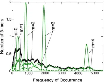
We explain the formulation presented in the last two sections by presenting results of distributions, or spectra, of frequency of 5-mers (as an example), and values of quantities such asffm,s2
m,fl, andCVfl2 for two genomes with very different base compositions: E. coli (p= 0.492) andC. acetobutylicum(p= 0.691). Here, a spectrum is the number of k-mers plotted against occurrence frequency. The spectra for the two genomes are shown as black curves in panels (A) and (B) of Fig. 9. The solid green curves characterized by narrow peaks are the spectra for random sequences obtained by scrambling the genomes. (The red curves are for sequences generated in the RSD model, see text.) In (A) the mean frequency of both spectra is
ff= 2|106/45= 1953. However, the genomic spectrum is seen to be much broader then the random-sequence spectrum, indicating that whereas in the random sequence frequencies (fu) of individual 5-mers deviate little from the mean (ff), in the genomic sequence that is not the case; frequencies of individual 5-mers fluctuate widely around the mean. Drastically different from (A), the overall widths of genome and random-sequence spectra in (B) are similar. Instead of having a single peak, the random-sequence spectrum is composed of six widely spread narrow subspectra whose peaks are near the theoretical mean frequencies (forp= 0.7) of them-sets,fff?g
m &152, 354, 827, 1930, 4500, 10500, form= 0 to 5, respectively. Eq. (6) shows that these mean values are determined bymand the base composition of the sequence, orp, and does not depend on the
Table 6.Average frequency of occurrence (ffm) of 5-mers in
p&0.5 andp&0.7 sequence.
fm
Sequence (m= ) 0 1 2 3 4 5
p~0:492
E. coli 2509 2245 1877 1760 1944 2656
Random 2101 2044 1987 1922 1857 1795
limL??Random 2114 2048 1983 1920 1860 1801
p~0:691
C. acetobutylicum 154 397 918 1951 4272 10300
Random 176 394 882 1970 4400 9832
limL??Random 176 393 880 1968 4402 9845
All sequences normalized to a length of 2 Mb;ff= 2|106/45= 1953. Random means matching random sequence, or sequence obtained by scrambling the genome.Values offff?g
m given by Eq. (6).
fluctuation of frequencies ofm-specific 5-mers. (B) and (C) in Fig. 9 show that in the random sequence frequency fluctuation within an m-set is again small. In contrast, and just as in (A), frequency fluctuations ofmspecific 5-mers in the genomic sequence are large (Fig. 9 (C) and Fig. 10 [70]).
Table 6 shows thatfff?g
m gives a very accurate estimate offfmfor random sequences and a fair one for genomic sequences. In the p= 0.492 case, the relation ffm&ff for all the m’s explains the narrowness of the random spectrum in Fig. 9 (A): like its counterpart in (B), it is also composed of six subspectra, but unlike (B) whose subspectra are spread widely, now the subspectra
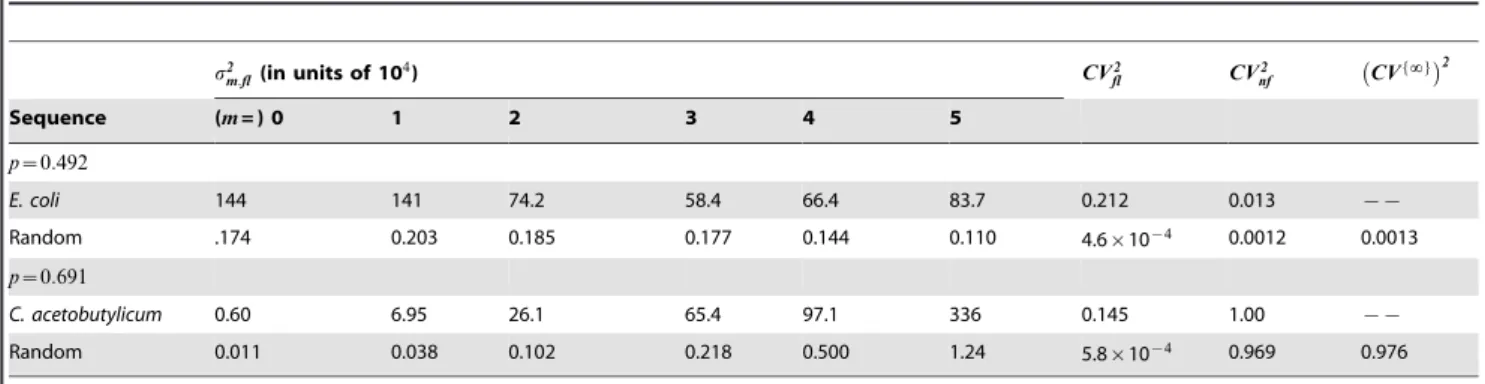
are superimposed. Table 7 highlight important aspects of our formulation: (i)CVnf has a strong dependence on pbut not on whether a sequence is genomic or random; (ii)CVf?g gives an
excellent estimate of CVnf for random sequences, and a fair estimate for genomes; (iii)CVfldepends weakly onpbut strongly on whether a sequence is genomic (relative large value) or random (several orders of magnitude smaller, and much smaller thanCVnf except whenp&0.5). (iv) For random sequences Eq. (13) is a fairly accurate relation.
Equivalent length
Thek-mers equivalent length of a sequence is defined as
le~bkt=CVfl2 (fork§2) ð14Þ
where CVfl2 is given by the frequency distribution of k-mers. Recalling that for a random sequence CVfl2 is inversely proportional sequence length (Eq. (13)), we see that le is the length of a random sequence whoseCVfl2has the same value as that of the genome. The empirical factorbk= 122{kz1, instead of the theoretical binomial factor 1{t{1, is used to ensure that for a random sequence, regardless of base composition,le approxi-mates the true sequence length with a high degree of accuracy. With the signal termCVflincluded but the stronglyp-dependence background termCVnf excluded in its definition,leis expected to have at most a weakp-dependence. That is,le is a quantity with which we can compare on the same footing genomes with widely disparate base compositions.
Genic, non-genic, exon, and intron concatenates These various concatenates are formed by splicing correspond-ing sections from a scorrespond-ingle strand of the DNA sequence and them stitching the sections together in the order and orientation they appear in the sequence. In particular, the genic and exon concatenates include genetic codes in positive and negative orientations.
Similarity index and similarity matrix
Given a pair of equal-length sequencesaandb, the similarity indexgsim(a,b)for the pair is defined as
g2sim(a,b)~ 1 kz1
X
m 1 2tm
X
u[Sm
(ffag
u {fufbg) 2
sfmagsfmbg
ð15Þ
whereSmis anm-set ands2mis the variance of the frequency of the k-mers in Sm. The pair are similar (in k-mer-content) when
gsim%1, are (considered to be) identical when gsim= 0, and are highly dissimilar whengsim 1. If we divideaandbinto (possibly overlapping) segments {a1,a2, } and {b1,b2, }, respectively, then we call the matrix whose element (i,j) is valuedgsim(ai,bj)a similarity matrix. In Fig. 6, similarity matrices are displayed as similarity plots by color coding elements of similarity matrices.
Minimum RSD model for genome growth
We denote byLthe designated length of a sequence andpthe designated AT-fraction of the sequence. We call the pair (L,p) theprofileof a sequence; in our model, the two profiles (L,p) and (L, 12p) are mathematically equivalent. By a growth model we mean a computer algorithm for generating, from an initial sequence, a target sequence that has a given profile and other specific genome-like attributes. Ours is a model of random
Figure 9. Frequency distributions of 5-mers.Frequency occur-rence distributions, or spectra, of 5-mers from the genomes of two prokaryotes, (A) E. coli (with (A+T) content p&0.5) and (B) C. acetobutylicum (p&0.7), normalized to a sequence length of 2 Mb. Abscissa give occurrence frequency and ordinates give number of 5-mers averaged, for better viewing, over a range of 21 frequencies to reduce fluctuation. The black, green and red curves represent spectra of the complete genomes, the randomized genome sequences and sequences generated in a model (see text), respectively. (C) Details of the m = 2 subspectra from (B).
doi:10.1371/journal.pone.0009844.g009
Figure 10. Frequency distributions of 5-mers inm-sets.Details of k= 5,m-specific subspectra from theC. acetobutylicumgenome (broken green curves) and matching random sequence (solid green curves); black curve is the same as in (B) Fig. 9. The five narrow subspectra peak (approximately) atfff?g
m , m= 0 to 4, or at 152, 354, 827, 1939, 4500,
respectively; them= 5 peak at 10500 is off scale (see Fig. 9 (B)). doi:10.1371/journal.pone.0009844.g010
segmental duplication (RSD) [49] in which the three main steps are: (i) randomly select a site from the sequence, (ii) from that site cull a segment of random length (but from a given length distribution) for duplication; (iii) reinsert the duplicated segment into the sequence at a (second) randomly selected site. The model has three explicit parameters:L0, the initial sequence length; dd, the average length of duplicated segments;r, the cumulative point mutation density (replacement only), or number of mutations per site. The generation of a model sequence involves three steps: selection of initial sequence, growth by RSD, point mutations. An initial sequence (of lengthL0) is chosen such that it has a target valuepbut is otherwise random. The lengthslof the duplicated segments are selected with uniform probability within the range 1 to 2dd, unless the current length of the genomeL’is less than 2dd, in which caselis selected from within the range 1 toL’. Growth is stopped when the length of the sequence exceeds the target length for the first time. Point mutations have a base bias defined bypand are administered after the growth is complete. That is, the administration of point mutations on the sequence is not meant to emulate point mutations suffered by a genome during its growth. Rather,ris meant to indicate the average cumulative number of point mutations per site experience by the genome throughout its life. Because RSD causes drifts in base composi-tion, the profile of the generated sequence will have a profile that is a close approximation of, but not exactly equal to, the target profile.
Mutation rates
We derive formulas for computing the rate density, or per site rate, of duplication events, mSD, and the rate density of ‘‘point mutation’’ – including small deletion and insertion but excluding SD – events,mp. If the genome grows from timet1to timet2at a rate proportional to its lengthl, that is,Dl=llDtwherelis the event rate (number of events per unit of time), then
l~(t2{t1) {1ln (l
2=l1), ð16Þ
If the grow is purely by SD and the average length of the duplicated segment isdd, then
mSD~l=dd: ð17Þ
If np is the cumulative number of point mutations, then
Dnp=mplDt. In SD dominated growth, the effect of point mutation on the overall length of a genome is negligible, so
integrating the relation yields
np(l2){np(l1)~mp(l2{l1)=l, ð18Þ
For anyl such that l&l1,np=mpl=l. The cumulative mutation sites is greater thannpbecause mutation sites are copied during
SD. The number of copied mutation sites satisfy
Dnc=npDl=l&mplDt (for largel). Therefore nc&np, that is, the cumulative number of mutated sites is twicenp. At full genome lengthL, this number isrL, hence
mp&rl=2: ð19Þ
Supporting Information
Figure S1 Category Le for coding and non-coding parts.
Averages ofp(fractional A/T-content) andLefork= 7 (situations for otherks are similar) for the coding parts (solid symbols;exfor eukaryotes andgnfor prokaryotes) and non-coding parts (hollow symbols;infor eukaryotes andigfor prokaryotes) of chromosomes. Symbols for categories are: vertebrates, red (square); unicellulars, blue (triangle-up); insects, orange (triangle-down); plants, green; prokaryotes, gray (bullet/circle). Numeral indicates number of chromosomes in each category. The curve represents Le for the universality class:Le{uc}(k;p).
Found at: doi:10.1371/journal.pone.0009844.s001 (0.26 MB TIF)
Figure S2 Distributions ofx2
versusLandp. Each symbol gives thex2
for one chromosomalLe. Top panels, for genic (gn) and exon (ex) concatenates. Bottom panels, for intergenic (ig) and intron (in) concatenates. Symbols, with color, number of data in group, and number of data whosex2is less than 1023given in brackets, stand
for: diamond, gn (blue; 7100; 229); square, ex (red; 2844, 95); triangle-down,ig(green; 6377, 270); triangle-up,in(orange; 2960, 104).
Found at: doi:10.1371/journal.pone.0009844.s002 (0.77 MB TIF)
Figure S3 Results from minimal RSD model. Top-left: Equi-x2
contour as function ofrandd, withL0= 64 (bases); length (L) of generated model sequence is 2 Mb and onlyLe(k) results fork= 7 are used. Top-right: Le(k), k= 2, 4, 6, 8, 10 from 200 model sequences generated using the ‘‘best’’ parameters L0= 64, ,d.= 1000 (b) and r= 0.73 (cumulative point mutations per base). The lines areLe{uc}(k;p) that represent the universality class Table 7.Values ofs’s from 5-mers inp&0.5 andp&0.7 sequences.
s2
m:fl (in units of 104) CVfl2 CVnf2 CVf
? ?g2
Sequence (m= ) 0 1 2 3 4 5
p~0:492
E. coli 144 141 74.2 58.4 66.4 83.7 0.212 0.013 {{
Random .174 0.203 0.185 0.177 0.144 0.110 4.6|10{4 0.0012 0.0013
p~0:691
C. acetobutylicum 0.60 6.95 26.1 65.4 97.1 336 0.145 1.00 {{
Random 0.011 0.038 0.102 0.218 0.500 1.24 5.8|10{4 0.969 0.976
All sequences normalized to a length of 2 Mb; fork= 5,ff= 1953,t= 1024, andtm= 32, 160, 320, 160, 32, form= 0 to 5.
given in the main text. Thex2
for the model sequences is 0.18. Bottom-left: x2 versus L0 (otherwise best parameters); model sequences haveL= 2 Mb and p= 0.5. Bottom-right: LeversusL, for ap= 0.5 model sequence generated using the best parameters. Found at: doi:10.1371/journal.pone.0009844.s003 (1.17 MB TIF)
Table S1 List of complete sequences included in the study (20
pp).
Found at: doi:10.1371/journal.pone.0009844.s004 (0.13 MB PDF)
Table S2 Equivalent lengths of complete sequences (100 pp).
Found at: doi:10.1371/journal.pone.0009844.s005 (0.36 MB PDF)
Table S3 Le(k), k= 2 to 10, averaged over categories of
organisms.
Found at: doi:10.1371/journal.pone.0009844.s006 (0.06 MB PDF)
Table S4 Leof sequences with highly biased compositions.
Found at: doi:10.1371/journal.pone.0009844.s007 (0.06 MB PDF)
Table S5 Effect of replication and segmental duplication onle.
Found at: doi:10.1371/journal.pone.0009844.s008 (0.04 MB PDF)
Text S1
Found at: doi:10.1371/journal.pone.0009844.s009 (0.07 MB PDF)
Author Contributions
Conceived and designed the experiments: HCL. Performed the experi-ments: HDC WLF SGK. Analyzed the data: HDC WLF SGK HCL. Wrote the paper: HCL.
References
1. Nei M, Li WH (1979) Mathematical model for studying genetic variation in terms of restriction endonucleases. Proc Natl Acad Sci U S A 76: 5269–5273. 2. Li WH (1997) Molecular Evolution Sinauer Associates: Sunderland, MA. 3. Ohno S (1970) Evolution by Gene Duplication Springer-Verlag: Berlin. 4. Hansche PE, Beres V, Lange P (1978) Gene duplication inSaccharomyces cerevisiae.
Genetics 88: 673–687.
5. Yamanaka K, Fang L, Inouye M (1998) The CSPA family inEscherichia coli: multiple gene duplication for stress adaptation. Mol Microbiol 27(2): 247–255. 6. Lynch M, Conery JS (2000) The evolutionary fate and consequences of duplicate
genes. Science 290: 1151–1155.
7. Gu Z, Steinmetz LM, Gu X, Scharfe C, Davis RW, et al. (2003) Role of duplicate genes in genetic robustness against null mutations. Nature 421: 63–66. 8. Zhang J (2003) Evolution by gene duplication: an update. Trends Ecol Evol
18(6): 292–298.
9. Lewin B (2000) Genes VII Oxford Univ Press. pp 89–115.
10. Lander ES, Linton LM, Birren B, Nusbaum C, Zody MC, et al. (2001) Initial sequencing and analysis of the human genome. Nature 409: 860–921. 11. Venter JC, Adams MD, Myers EW, Li PW, Mural RJ, et al. (2001) The
sequence of the human genome. Science 291: 1304–1351.
12. Kleckner N (1981) Transposable elements in prokaryotes. Ann Rev Genet 15: 341–404.
13. Castilho BA, Olfson P, Casadaban MJ (1984) Plasmid insertion mutagenesis and lac gene fusion with mini-mu bacteriophage transposons. J Bacteriol 158(2): 488–495.
14. Levis RW, Ganesan R, Houtchens K, Tolar LA, Sheen FM (1993) Transposons in place of telomeric repeats at aDrosophilatelomere. Cell 75(6): 1083–1093. 15. Li WH, Gojobori T, Nei M (1981) Pseudogenes as a paradigm of neutral
evolution. Nature 292: 237–239.
16. Vanin EF (1985) Processed pseudogenes: Characteristics and evolution. Annu Rev Genet 19: 253–272.
17. Weiner AM, Deininger PL, Efstratiadis A (1986) Nonviral retroposons: genes, pseudogenes, and trans- posable elements generated by the reverse flow of genetic information. Annu Rev Biochem 55: 631–661.
18. Bensasson D, Zhang DX, Hartl DL, Hewitt GM (2001) Mitochondrial pseudogenes: evolution’s misplaced witnesses. Trends Ecol Evol 16(6): 314–321. 19. McGrath JM, Jancso MM, Pichersky E (1993) Duplicate sequences with a similarity to expressed genes in the genome ofArabidopsis thaliana. Theor Appl Genet 86: 880–888.
20. Bailey JA, Yavor AM, Massa HF, Trask BJ, Eichler EE (2001) Segmental duplications: Organization and impact within the current human genome project assembly. Genome Res 11: 1005–1017.
21. Bailey JA, Gu Z, Clark RA, Reinert K, Samonte RV, et al. (2002) Recent segmental duplications in the human genome. Science 297: 1003–1007. 22. Sharp AJ, Locke DP, McGrath SD, Cheng Z, Bailey JA, et al. (2005) Segmental
duplications and copy-number variation in the human genome. Am J Human Genet 77: 78–88.
23. Gaut BS, Doebley JF (1997) DNA sequence evidence for the segmental allotetraploid origin of maize. Proc Natl Acad Sci U S A 94: 6809–6814. 24. Gale MD, Devos KM (1998) Comparative genetics in the grasses. Proc Natl
Acad Sci U S A 95: 1971–1974.
25. Mochizuki K, Fine NA, Fujisawa T, Gorovsky MA (2002) Analysis of a piwi-related gene implicates small RNAs in genome rearrangement inTetrahymena. Cell 110: 689–699.
26. Coghlan A, Wolfe KH (2002) Fourfold faster rate of genome rearrangement in nematodes than inDrosophila. Genome Res 12: 857–867.
27. Pevzner P, Tesler G (2003) Genome rearrangements in mammalian evolution: Lessons from human and mouse genomes. Genome Res 13: 37–45.
28. Grant D, Cregan P, Shoemaker RC (2000) Genome organization in dicots: Genome duplication inArabidopsisand synteny between soybean andArabidopsis. Proc Natl Acad Sci U S A 97: 4168–4173.
29. Spring J (2002) Genome duplication strikes back. Nat Genet 31: 128–129. 30. Kellis M, Birren BW, Lander ES (2004) Proof and evolutionary analysis of
ancient genome dupli- cation in the yeastSaccharomyces cerevisiae. Nature 428: 617–624.
31. Peng CK, Buldyrev SV, Goldberg AL, Havlin S, Simons M, et al. (1993) Finite-size effects on long-range correlations: Implications for analyzing DNA sequences. Phys Rev E 47: 3730–3733.
32. Mantegna RN, Buldyrev SV, Goldberger AL, Havlin S, Peng CK, et al. (1994) Linguistic features of noncoding DNA sequences. Phys Rev Lett 73: 3169–3172. 33. Forsdyke D (1995) Relative roles of primary sequence and (G+C)% in determining the hierarchy of frequencies of complementary trinucleotide pairs in DNAs of different species. J Mol Evol 41: 573–581.
34. Karlin S, Mrazek J (1997) Compositional differences within and between eukaryotic genomes. Proc Natl Acad Sci U S A 94: 10227–10232.
35. Deschavanne PJ, Giron A, Vilain J, Fagot G, Fertil B (1999) Genomic signature: characterization and classiffication of species assessed by chaos game representation of sequences. Mol Biol Evol 16(10): 1391–1399.
36. Hao BL, Lee HC, Zhang SY (2000) Fractals related to long DNA sequences and complete genomes. Chaos, Solitons and Fractals 11: 825–836.
37. Ochman H, Elwyn S, Moran NA (1999) Calibrating bacterial evolution. Proc Natl Acad Sci U S A 96: 12638–12643.
38. Nachman MW, Crowell SL (2000) Estimate of the mutation rate per nucleotide in humans. Genetics 156: 297–304.
39. Liu G, Program NCS, Zhao S, Bailey JA, Sahinalp SC, et al. (2003) Analysis of primate genomic variation reveals a repeat-driven expansion of the human genome. Genome Res 13: 358–368.
40. Voss RF (1996) Comment on ‘‘Linguistic features of noncoding DNA sequences’’. Phys Rev Lett 76: 1978.
41. Bonhoeffer S, Herz AV, Boerlijst MC, Nee S, Nowak MA, et al. (1996) No signs of hidden language in noncoding DNA. Phys Rev Lett 76: 1977.
42. Israeloff NE, Kagalenko M, Chan K (1996) Can Zipf distinguish language from noise in noncoding DNA? Phys Rev Lett 76: 1976.
43. Mantegna RN, Buldyrev SV, Goldberger AL, Halvin S, Peng CK, et al. (1996) Mantegna et al. reply:. Phys Rev Lett 76: 1979–1981.
44. Peng CK, Buldyrev SV, Havlin S, Simons M, Stanley HE, et al. (1994) Mosaic organization of DNA nucleotides. Phys Rev E 49: 1685–1689.
45. Bernaola-Galvffan P, Carpena P, Roman-Roldan R, Oliver JL (2002) Study of statistical correlations in DNA sequences. Gene 300: 105–115.
46. Messer PW, Arndt PF, Lassig M (2005) Solvable sequence evolution models and genomic correlations. Phys Rev Lett 94: 138103.
47. Fickett JW, Torney DC, Wolf DR (1992) Base compositional structure of genomes. Genomics 13: 1056–1064.
48. Xie HM, Hao BL (2002) Visualization of k-tuple distribution in procaryote complete genomes and their randomized counterparts. In: Proceedings of the IEEE Computer Society Bioinformatics Conference. pp 31–42.
49. Hsieh LC, Luo LF, Lee HC (2003) Genomes are large systems with small-system statistics: Seg- mental duplication in the growth of microbial chromosomes. AAPPS Bulletin 13: 22–27.
50. Chen TY, Hsieh LC, Lee HC (2005) Shannon information and self-similarity in complete chromosomes. Comput Phys Commun 169: 218–221.
51. Zhou F, Olman V, Xu Y (2008) Barcodes for genomes and applications. BMC Bioinformatics 9: 546.
52. Kong SG, Chen HD, Fan WL, Wigger J, Torda AE, et al. (2009) Quantitative measure of random- ness and order for complete genomes. Phys Rev E 79: 061911.