Modeling rapid mass movements using the shallow water equations

(1)

NHESSD

2, 6775–6809, 2014

Modeling rapid mass movements using the

shallow water equations

S. Hergarten and J. Robl

Title Page

Abstract Introduction

Conclusions References

Tables Figures

◭ ◮

Back Close

Full Screen / Esc

Printer-friendly Version Interactive Discussion

Discussion

P

a

per

|

Discus

sion

P

a

per

|

Discussion

P

a

per

|

Discussion

P

a

per

|

Nat. Hazards Earth Syst. Sci. Discuss., 2, 6775–6809, 2014 www.nat-hazards-earth-syst-sci-discuss.net/2/6775/2014/ doi:10.5194/nhessd-2-6775-2014

This discussion paper is/has been under review for the journal Natural Hazards and Earth System Sciences (NHESS). Please refer to the corresponding final paper in NHESS if available.

Modeling rapid mass movements using

the shallow water equations

S. Hergarten1and J. Robl2

1

Universität Freiburg i. Br., Institut für Geo- und Umweltnaturwissenschaften, Freiburg, Germany

2

Universität Salzburg, Institut für Geographie und Geologie, Salzburg, Austria

Received: 29 September 2014 – Accepted: 13 October 2014 – Published: 4 November 2014 Correspondence to: J. Robl (joerg.robl@sbg.ac.at)

(2)

NHESSD

2, 6775–6809, 2014

Title Page

Tables Figures

◭ ◮

Back Close

Full Screen / Esc

Discussion

P

a

per

|

Discus

sion

P

a

per

|

Discussion

P

a

per

|

Discussion

P

a

per

|

Abstract

We propose a new method to model rapid mass movements on complex topography using the shallow water equations in Cartesian coordinates. These equations are the widely used standard approximation for the flow of water in rivers and shallow lakes, but the main prerequisite for their application – an almost horizontal fluid table – is in

5

general not satisfied for avalanches and debris flows in steep terrain. Therefore, we have developed appropriate correction terms for large topographic gradients. In this study we present the mathematical formulation of these correction terms and their im-plementation in the open source flow solver GERRIS. This novel approach is evaluated by simulating avalanches on synthetic and finally natural topographies and the widely

10

used Voellmy flow resistance law. The results are tested against analytical solutions and the commercial avalanche model RAMMS. The overall results are in excellent

agreement with the reference system RAMMS, and the deviations between the diff

er-ent models are far below the uncertainties in the determination of the relevant fluid parameters and involved avalanche volumes in reality. As this code is freely available

15

and open source, it can be easily extended by additional fluid models or source areas, making this model suitable for simulating several types of rapid mass movements. It therefore provides a valuable tool assisting regional scale natural hazard studies.

1 Introduction

Rapid mass movements such as avalanches, debris flows, and lahars are globally

20

abundant surface processes in steep mountainous areas characterized by high process velocities and large masses of granular material involved (e.g. Kirschbaum et al., 2010). Therefore, rapid mass movements represent first-order threats whenever their process domains intersect with populated areas and infrastructure for transport (streets, rail-way lines), energy supply (power plants, pipelines, electricity lines) or tourism (e.g.

25

(3)

NHESSD

2, 6775–6809, 2014

Title Page

Tables Figures

◭ ◮

Back Close

Full Screen / Esc

Discussion

P

a

per

|

Discus

sion

P

a

per

|

Discussion

P

a

per

|

Discussion

P

a

per

|

implemented hazard mitigation strategies by a combination of permanent and temporal preventive measures, the latter are progressively developed in remote mountainous re-gions where historical records on rapid mass movements are sparse, so that the level of threat is ambiguous. In combination with field mapping and remote sensing, numer-ical models describing the motion of granular material on general topography are the

5

primary tool to evaluate the potential impact of rapid mass movements on infrastruc-ture in these remote places. Runout distance, flow and depositional depth, velocity, and momentum of a granular flow resulting from physically based numerical models represent key parameters to (a) delineate hazard zones on regional scale, (b) locate ideal corridors and construction areas for new infrastructure, and (c) develop

mitiga-10

tion strategies for protecting planned and already existing infrastructure against these natural hazards (Hsu et al., 2010; Keiler et al., 2006). To fulfill these tasks codes have to be equipped with advanced numerical techniques to reach the required computa-tional performance (e.g. adaptive mesh refinement), have to provide an interface to geographic information systems (GIS) and should be controllable by a scripting

lan-15

guage to perform Monte Carlo simulations and parameter studies for entire valleys and hundreds of process domains.

Several state-of-the-art codes describe granular flow on general topography, but are either not open source (e.g. FLATModel, Medina et al., 2008) or restricted to simple Coulomb-type rheology (e.g. Titan2D, Sheridan et al., 2005). The implementation of

20

a new rheology model even in open-source scientific codes by the user is in general not practicable as a deep knowledge on the specific code and fluid dynamics is re-quired. Other recent codes such as Flow-R (Horton et al., 2013) replace the equations of continuum mechanics by more empirical, grid-based algorithms and thus require a higher degree of calibration.

25

The Voellmy rheology (Voellmy, 1955) is commonly used to describe debris flows

and dense snow avalanches and is implemented in different flavors in commercial

software products such as RAMMS (Christen et al., 2010), SAMOS-AT (Sampl and

(4)

NHESSD

2, 6775–6809, 2014

Title Page

Tables Figures

◭ ◮

Back Close

Full Screen / Esc

Discussion

P

a

per

|

Discus

sion

P

a

per

|

Discussion

P

a

per

|

Discussion

P

a

per

|

been extensively used by the Austrian avalanche and torrent control, but peer-reviewed publications on technical details are still missing. Astonishingly, there are no open-source codes that fulfill all requirements mentioned above to describe granular flow with a Voellmy rheological model on complex topography. In return, there are several open-source packages for a wide range of fluid dynamical problems that provide

state-5

of-the-art flow solvers and a variety of numerical accessories like automatic meshing routines or adaptive mesh refinement, such as OPENFOAM (Weller and Weller, 2008, http://www.openfoam.com), CLAWPACK (LeVeque et al., 2011; Berger et al., 2011, http://clawpack.github.io), and GERRIS (Popinet, 2009, http://gfs.sourceforge.net). Be-side many other applications these codes are routinely used to predict the propagation

10

of tsunamis in ocean basins (Popinet, 2012) or to model the extent of inundation areas during flooding (An and Yu, 2012) by solving the nonlinear shallow water equations be-ing the standard approximation for the flow of water in rivers and shallow lakes. These numerical packages are operated by highly flexible parameter files that allow the im-plementation of new fluid rheology models without writing additional source code, so

15

that it is tempting to describe rapid mass movements with one of these fluid dynamics software packages.

In their spirit, two-dimensional models for rapid mass movements on a given topog-raphy are similar to the shallow water equations. In both concepts, vertically averaged

velocities are considered, and the rheology of the medium and effects of turbulence

20

are taken into account in form of a friction term depending on flow depth and velocity. However, the widely used shallow water equations are only applicable if the water table is almost horizontal. This condition is in general not satisfied for mass movements in steep terrain, so that more elaborate approaches are required here.

These approaches can be subdivided into two major classes according to the

coor-25

(5)

NHESSD

2, 6775–6809, 2014

Title Page

Tables Figures

◭ ◮

Back Close

Full Screen / Esc

Discussion

P

a

per

|

Discus

sion

P

a

per

|

Discussion

P

a

per

|

Discussion

P

a

per

|

thalweg in downslope direction (red). A formulation for granular flow in general curved and twisted channels was provided by Pudasaini and Hutter (2003). Recently, an im-plementation of this concept called r.avalanche in the Open Source GIS GRASS was presented by Mergili et al. (2012). However, it imposes significant simplifications to the thalweg concept, in particular that it is a straight line in map view, so that it is more

5

suitable for flow on slopes than in pre-defined channels. The alternative concept only

assumes that the z coordinate is normal to the surface, while the horizontal

projec-tions of x and y coordinates approximately follow the original Cartesian axes (blue).

The software RAMMS (Christen et al., 2010) implements the simplest version of such a local coordinate system by neglecting the surface curvature. An extension taking the

10

surface curvature into account for the price of more complicated di_fferential equations was presented by Fischer et al. (2012).

In this paper we introduce a different approach based on the original shallow water

equations in Cartesian coordinates. Instead of the velocity parallel to the surface, the horizontal component is computed and converted to the velocity parallel to the surface

15

afterwards. The basic problem of this approach, an overestimation of the acceleration, is compensated by introducing an appropriate friction term. In the following section, an expression for this friction term is derived, and in Sect. 4 the approach is validated by comparing several scenarios with the established avalanche model RAMMS.

2 Theory

20

The shallow water equations provide a two-dimensional approximation for the flow of water (or any liquid or granular medium). They refer to vertically averaged horizontal velocities and assume an almost horizontal water table, so that the vertical component of the velocity can be neglected, and the vertical pressure distribution is hydrostatic. Under these conditions, the horizontal pressure gradient and thus the horizontal

ac-25

(6)

NHESSD

2, 6775–6809, 2014

Title Page

Tables Figures

◭ ◮

Back Close

Full Screen / Esc

Discussion

P

a

per

|

Discus

sion

P

a

per

|

Discussion

P

a

per

|

Discussion

P

a

per

|

equation

∂

∂tvh+(vh· ∇)vh=gs− τ ρh_v

v_h

|v

h|

(1)

with

s=−∇(H+h_v). (2)

The model variables are the vertically averaged horizontal velocity v_h (a

two-5

component vector) and the vertical (not normal to the surface) flow depth h_v. Both

variables depend on the spatial coordinatesx and y and on time. The symbol∇

de-notes the two-dimensional gradient operator, andH(x,y) is the topography, so thatsis

the negative gradient of the water table. The parametersgandρare the gravitational

acceleration and the density, respectively. The second term at the right-hand side is

10

a friction term in direction opposite to the velocity. Here it is written in terms of a basal shear stressτ, but this does not imply that friction in fact only occurs at the bottom of the fluid layer. For turbulent flow of water,τis proportional to the square of the velocity, but arbitrary functions involving velocity and flow depth may be used.

If the gradient of the water table is large, the corresponding acceleration term

overes-15

timates the real acceleration for two reasons: (i) the real acceleration acts in direction parallel to the surface, while Eq. (1) involves only its horizontal component. (ii) The absolute value of the gradient of the water table,|s|, corresponds to the tangent of the

slope angleϕ,

tanϕ₌|s|, (3)

20

while the downslope acceleration on an inclined plane is in fact proportional to sinϕ.

(7)

NHESSD

2, 6775–6809, 2014

Title Page

Tables Figures

◭ ◮

Back Close

Full Screen / Esc

Discussion

P

a

per

|

Discus

sion

P

a

per

|

Discussion

P

a

per

|

Discussion

P

a

per

|

The friction term also requires a correction for finite gradients, namely a multiplication by cosψwhereψ is the inclination angle of the velocity. This angle is in general smaller thanϕand only equal to it for flow in downslope direction. It is given by

tanψ₌

v

h·s

|v

h|

. (4)

Furthermore, the vertical flow depthh_v must be replaced by the flow depth normal to

5

the surface that is by a factor cosϕ smaller. Returning to the vertical flow depth h_v

requires the division of the friction term by cosϕ.

With these three modifications to the right-hand side, the shallow water equations turn into

∂

∂tvh+(vh· ∇)vh=gcos

2_ϕ_s₋ τ

ρh_v

cosψ

cosϕ

v_h

|v_h|

. (5)

10

It should be mentioned that these modifications only extract the vertical components of the acceleration terms at the right-hand side, but do not correct the terms of inertia due to surface curvature.

As our approach shall be compatible with the original shallow water equations, the acceleration term shall remain linear, so that the reduction of the acceleration must be

15

mimicked by an additional friction term

a₌_gcos2_ϕs−_gs (6)

=−gsin2ϕs. (7)

However, the original shallow water equations only allow a friction term in direction

20

(8)

NHESSD

2, 6775–6809, 2014

Title Page

Tables Figures

◭ ◮

Back Close

Full Screen / Esc

Discussion

P

a

per

|

Discus

sion

P

a

per

|

Discussion

P

a

per

|

Discussion

P

a

per

|

velocity,

a=−gsin2ϕs· v

h

|v_h| v

h

|v_h| (8)

=−gsin2ϕtanψ

v_h

|v_h|, (9)

while the component normal to the flow direction is neglected. With this approximation,

5

Eq. (5) turns into

∂

∂tvh+(vh· ∇)vh=gs−

gsin2ϕtanψ₊ τ ρh_v

cosψ

cosϕ

_v

h

|v

h|

. (10)

In the context of dense snow avalanches, the Voellmy rheology (Voellmy, 1955) is the most widely used constitutive law for the friction term. It combines a velocity-independent Coulomb friction term with a term proportional to the square of the velocity

10

as it is mostly used for turbulent flow:

τ₌µσ₊ρgv

2

ξ (11)

Here,σ denotes the normal stress at the bottom of the fluid layer. Assuming that the

bottom is parallel to the surface, it is given by

σ₌ρgh_vcos2ϕ. (12)

15

The second term at the right-hand side of Eq. (11) is independent of the direction of the velocity, so that we obtain

τ₌µρgh_vcos2ϕ₊ ρg|

v

h| 2

(9)

NHESSD

2, 6775–6809, 2014

Title Page

Tables Figures

◭ ◮

Back Close

Full Screen / Esc

Discussion

P

a

per

|

Discus

sion

P

a

per

|

Discussion

P

a

per

|

Discussion

P

a

per

|

Inserting this expression in Eq. (10) finally yields

∂

∂tvh+(vh· ∇)vh=gs−g sin

2_ϕ

tanψ₊µcosϕcosψ₊ |vh|

2

ξh_vcosϕcosψ

! v_h

|v_h|

. (14)

This set of equations differs from the original shallow water equations (Eq. 1) only by the more complicated friction term (the expression in parentheses at the right-hand side).

5

3 Implementation

Our approximation can easily be implemented in any continuum fluid dynamics soft-ware which is able to solve the shallow water equations for a given bed topography and allows the implementation of arbitrary friction terms. We use the software package GERRIS (http://gfs.sourceforge.net) which is freely available and has been developed

10

for more than ten years. It provides highly developed numerics, and applications of GERRIS have been presented in numerous publications.

Operator splitting provides the simplest way of implementing a nonlinear friction term as the one in Eq. (14). Let us write Eq. (14) in the form

∂

∂tvh+(vh· ∇)vh=gs−f(hv,vh,ϕ,ψ)vh (15)

15

with

f(h_v,v_h,ϕ,ψ)=

g

sin2ϕtanψ₊µcosϕcosψ₊ |vh|2 ξh_vcosϕcosψ

|v_h|

. (16)

(10)

NHESSD

2, 6775–6809, 2014

Title Page

Tables Figures

◭ ◮

Back Close

Full Screen / Esc

Discussion

P

a

per

|

Discus

sion

P

a

per

|

Discussion

P

a

per

|

Discussion

P

a

per

|

solving the shallow water equations without friction. In the second half step, the “real” velocity at the time t₊δt is computed from ˜v_h, ˜h_v, ˜ϕ, and ˜ψ by applying the friction

term only, i.e. by solving the differential equation

∂

∂tvh=−f(hv,vh,ϕ,ψ)vh (17)

where the solution at the time t is the interim velocity ˜v_h. As this equation does not 5

contain any spatial derivatives of the velocity, it is degenerated to a set of ordinary differential equations. Furthermore it does not alter the direction of v

h, so that it is in

principle even scalar. Applying a mixed Euler scheme with an explicit discretization of the arguments off and an implicit discretization to the remaining termv_h, i.e.

v_h(t+δt)−v˜_h

δt =−f( ˜hv, ˜vh, ˜ϕ, ˜ψ)vh(t+δt) (18)

10

yields the solution

v_h= ˜

v_h

1+δtf( ˜h_v, ˜v_h, ˜ϕ, ˜ψ)

. (19)

The angles ˜ϕand ˜ψshould be computed from the gradient of the surface of the flowing medium (Eq. 2) according to Eqs. (3) and (4) in each timestep. However, the shallow water equations are in principle only valid as long as the gradient of the flow depth is

15

small, i.e. as long as the flow surface is almost parallel to the topography. The correc-tions introduced in Sect. 2 indeed refer to the inclination of the flow surface, except for the normal stress responsible for the static friction term (Eq. 12) that should rather be related to the topography of the bottom. So in sum, using the gradient of the flow surface should be better than using the gradient of the topography, but practically the

20

(11)

NHESSD

2, 6775–6809, 2014

Title Page

Tables Figures

◭ ◮

Back Close

Full Screen / Esc

Discussion

P

a

per

|

Discus

sion

P

a

per

|

Discussion

P

a

per

|

Discussion

P

a

per

|

in Sect. 4.1, using the gradient of the flow surface may even generate artefacts if this gradient is not computed from the same discretization scheme that is used internally for solving the shallow water equations, which will likely occur when staggered grids or finite volume discretizations are used. Under this aspect it may be even advisable to use the topographic gradient.

5

4 Validation

In this section we compare our approximation to the established model RAMMS. We use the simplest version based on Voellmy’s rheology, neglecting entrainment (Christen et al., 2010) and do not use the recently introduced features of extending Voellmy’s

rheology by cohesion and taking into account the effect of surface curvature on the

10

frictional force considered by Fischer et al. (2012). However, all these extensions can in principle be adjusted to our formulation based on the shallow water equations in Cartesian coordinates.

Compared to the reference model RAMMS as defined above, our approach intro-duces two approximations. The most serious one consists in considering only the

hori-15

zontal component of the velocity. While the accelerations due to the slope gradient and due to friction are corrected accordingly, the horizontal velocity would remain constant in absence of gravity or friction. As a consequence, the total velocity increases artifi-cially on a convex slope and decreases on a concave slope even without gravitational acceleration. The other simplification concerns applying the correction in acceleration

20

for large slope gradients only in flow direction while leaving the lateral acceleration uncorrected.

In the following we investigate three scenarios defined with regard to these approx-imations. In the first example, flow down a planar slope is considered. This scenario should be described well by both RAMMS and by our approach. The second set of

25

(12)

NHESSD

2, 6775–6809, 2014

Title Page

Tables Figures

◭ ◮

Back Close

Full Screen / Esc

Discussion

P

a

per

|

Discus

sion

P

a

per

|

Discussion

P

a

per

|

Discussion

P

a

per

|

approximation has a serious effect. Finally we consider a more complex topography as

an example being closer to real-world applications.

4.1 Constant flow depth on a planar slope

The movement of an avalanche with a constant flow depth on a planar slope in one dimension can be described by an analytical solution. For this purpose we use the

5

velocityv parallel to the slope and Lagrangian coordinates, which means thatv is the

velocity of a given particle and not at a given position. Then the equation of motion is the same as for a rigid body,

∂v

∂t =gsinϕ− τ

ρh, (20)

whereτis the frictional shear stress. According to the arguments leading from Eq. (11)

10

to Eq. (13), this shear stress amounts to

τ₌µρghcosϕ₊ρgv

2

ξ , (21)

so that

∂v

∂t =g sinϕ−µcosϕ− v2 ξh

!

. (22)

The steady-state solution of this equation (i.e. the asymptotic velocity v_∞) is readily

15

obtained by setting the left-hand side to zero:

v_∞₌

q

ξh(sinϕ−µcosϕ) (23)

With this, Eq. (22) turns into

∂v ∂t =

g ξh

(13)

NHESSD

2, 6775–6809, 2014

Title Page

Tables Figures

◭ ◮

Back Close

Full Screen / Esc

Discussion

P

a

per

|

Discus

sion

P

a

per

|

Discussion

P

a

per

|

Discussion

P

a

per

|

The time-dependent solution of this equation is

v₌v_∞tanh

t T

(25)

with the characteristic time

T= ξh

gv_∞ (26)

describing how slowly the velocity approachesv_∞.

5

For testing whether our approach reproduces this behavior correctly, we consider

a planar ramp withϕ₌30◦ inclination inx direction with Voellmy parametersµ₌0.2

andξ₌1000 m s−2. The release zone is defined by a rectangular area of 350 m×400 m (in horizontal projection) at the upper edge of the ramp with a release height ofh₌1 m measured normal to the topography. Figure 2a shows the topography and the flow

10

depth after 20 s obtained from the simulation with GERRIS where the frictional terms

(i.e. the anglesϕandψ in Eq. 14) are computed from the surface of the flowing mass.

According to the notation in the GERRIS parameter files, this realization is denoted

GERRISHin the following.

Figure 2b compares the longitudinal avalanche profiles of flow depth and flow

ve-15

locity obtained from three different numerical experiments: the realization GERRISH

discussed above, the alternative approach where the bed surface (i.e. the original

to-pography) is used to compute the friction term (denoted GERRIS_Zb in the following),

and the reference model RAMMS. Only minor differences between the three models

are encountered. The avalanche develops a characteristic tail with a rapidly

declin-20

ing flow depth in up-slope direction, while the initial flow depth ofh₌1 m is still pre-served in the main body. The avalanche has already reached the steady-state velocity

of about 18 m s−1 in the main body predicted by Eq. (23), while the velocities in the

tail are lower as a consequence of the reduced flow depth. The avalanche front of all three experiments is characterized by a slight increase of flow depth and flow velocity

(14)

NHESSD

2, 6775–6809, 2014

Title Page

Tables Figures

◭ ◮

Back Close

Full Screen / Esc

Discussion

P

a

per

|

Discus

sion

P

a

per

|

Discussion

P

a

per

|

Discussion

P

a

per

|

relative to the main avalanche body. This artefact is in general small, but most

pro-nounced for GERRISH, while RAMMS and GERRISZb show nearly identical profiles at

the avalanche front. The slightly stronger artefact occurring in GERRISH presumably

arises from our simple implementation of the gradient of the fluid surface required for

computing the anglesϕand ψ required in Eq. (19). Here we use the standard

gradi-5

ent of the fluid surface provided by GERRIS that is computed from simple symmetrical

difference quotients. The sophisticated numerics implemented in GERRIS itself used

for maintaining a sharp front is not incorporated here, so that finally the driving term of

the shallow water equations and the friction term use different schemes of

discretiza-tion, causing artefacts at the avalanche front where the fluid surface is strongly curved.

10

However, we found in all considered examples that these small artefacts are stable and do not grow through time, so that they are not a serious problem at all.

As a second test, we consider the velocity of the accelerating fluid layer against the time dependent analytical solution (Eq. 25) for di_fferent initial flow depths (h), turbu-lence (ξ) and dry friction (µ) parameters of the Voellmy rheology, and hillslope angles

15

(ϕ) (Fig. 3). Similarly to the results on the avalanche profiles, the almost perfect agree-ment between the velocity predicted by Eq. (25) and all sets of numerical experiagree-ments verifies the ability of our approach at least for planar slopes. Small deviations occur-ring shortly after the release scale with the time step size of the numerical model and could be reduced by forcing the flow solver towards smaller time increments. However,

20

these initial small deviations disappear rapidly when approaching the terminal velocity, so that a higher temporal resolution at the expense of increasing computational time does not justify this insignificant benefit in practical applications.

4.2 The effect of profile curvature

While the tests performed in the previous section only concern the technical

correct-25

(15)

NHESSD

2, 6775–6809, 2014

Title Page

Tables Figures

◭ ◮

Back Close

Full Screen / Esc

Discussion

P

a

per

|

Discus

sion

P

a

per

|

Discussion

P

a

per

|

Discussion

P

a

per

|

In order to explore the effects of profile curvature on our approach considering only the horizontal components of the velocity vector (and calculating the total velocity from those) we have performed a series of numerical experiments on curved synthetic to-pographies and confront the results of our approach with those of RAMMS. The first

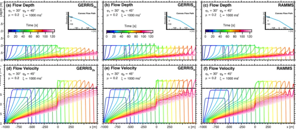
experiment describes an avalanche on a concave flow path defined by a 30◦ dipping

5

ramp and a 5◦inclined runout zone with a smooth transition between both (Fig. 4). Here and in the following the curvature of the smooth transition zone is defined in such a way that an avalanche entering from the upper ramp with the terminal velocity according to Eq. (23) is exposed to an centrifugal acceleration of about 1 m s−2(which is neglected in both RAMMS and our approach, but considered in detail by Fischer et al., 2012).

10

The behavior when traveling along the upper ramp is the same as in the example

considered in Fig. 2. At t₌40 s, the avalanche is characterized by a long tail, while

the bulk mass of the avalanche remains undeformed and has reached the steady-state velocity of about 18 m s−1(Fig. 4c and d). At this time the avalanche front approaches the curved transition zone to the gently dipping runout zone leading to a strong

decel-15

eration and thickening. Att₌60 s, the frontal part of the fluid layer is more than three times thicker than it initially was. The flow velocity has decreased below 10 m s−1

ev-erywhere (Fig. 4e and f). Att₌80 s, the avalanche thickens further in the runout zone

and grows laterally normal to the flow path and in upslope direction as additional mass from the slower avalanche tail becomes incorporated in the deposit. At this stage,

sig-20

nificant flow velocities are confined to the steep flow path section where the avalanche tail is still in motion (Fig. 4g and h).

While Fig. 4 shows that the avalanche behaves as expected qualitatively, Fig. 5 pro-vides a quantitative comparison with the reference model RAMMS. The flow depths (Fig. 5a–c) and the velocities (Fig. 5d–f) predicted by both models agree almost

per-25

(16)

NHESSD

2, 6775–6809, 2014

Title Page

Tables Figures

◭ ◮

Back Close

Full Screen / Esc

Discussion

P

a

per

|

Discus

sion

P

a

per

|

Discussion

P

a

per

|

Discussion

P

a

per

|

Noticeable differences between the results of the GERRIS-based models and

RAMMS only occur in the final phase of the avalanche when the front has almost come to rest. While the main body of the avalanche is characterized by a single max-imum in the thickness in the GERRIS-based simulations, RAMMS predicts a bimodal avalanche profile. This difference is also reflected in the shape of the final deposits at

5

least when the RAMMS simulation is stopped automatically using the default settings (i.e. when the momentum has decreased to 5 % of its maximum value). However, the difference arises in a phase where only the long tail of the avalanche moves at a con-siderable velocity, so that material is pushed from behind on the main avalanche body that is almost resting. So this difference is probably not related to the different way of

10

treating velocities, but rather to the di_fferent numerical schemes used in RAMMS and

GERRIS, and apart from this unimportant for practical purposes.

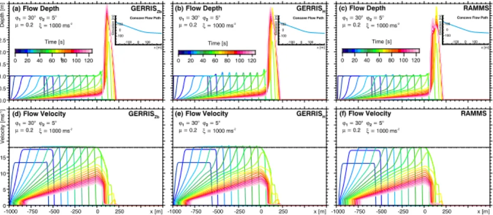
In Fig. 6, the opposite situation involving a convex topography is considered. Again the release zone is located on a 30◦steep slope, but in contrast to the previous exper-iment the slope steepens in a smooth transition to 45◦. The transition from ϕ₁₌30◦

15

toϕ₂₌45◦ causes the fluid layer to accelerate rapidly from 18 m s−1 to the new

ter-minal velocity of 21.7 m s−1 at a reduced flow depth of 0.83 m. As an effect of our

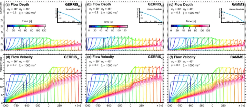
approximation considering only the horizontal components of the velocity vector, the new terminal velocity is reached slightly earlier by GERRIS than by RAMMS. This ef-fect becomes more pronounced by sharp terrain transitions (Fig. 7). In this example,

20

the sharp transition from ϕ₁₌30◦ to ϕ₂₌45◦ increases the velocity instantaneously to 18 m s−1×cos 30_{cos 45}◦◦ =22 m s

−1

, which is even slightly above the new terminal veloc-ity. However, the avalanche of RAMMS reaches the terminal velocity also rapidly after entering the 45◦slope for both the smooth and the sharp transition.

A quantitative estimate on the range where our approximation affects the flow velocity

25

(17)

NHESSD

2, 6775–6809, 2014

Title Page

Tables Figures

◭ ◮

Back Close

Full Screen / Esc

Discussion

P

a

per

|

Discus

sion

P

a

per

|

Discussion

P

a

per

|

Discussion

P

a

per

|

a function of the traveled distance. Using Eq. (24) we obtain

∂v ∂x =

∂v ∂t ∂x ∂t

=

g ξh

v_∞2 −v2

v (27)

≈2g

ξh(v∞−v) forv≈v∞. (28)

Equation (28) implies that v approaches the terminal velocity v_∞ exponentially with

5

a decay length

L₌ ξh

2g. (29)

In the example considered above, L amounts to about 42 m, so that the avalanche

indeed needs a very short traveling distance to approach the terminal velocity. Con-sidering the more realistic situation of a steady-state avalanche with a constant influx

10

instead of a constant flow depth, i.e. hv ₌const, leads to basically the same result

where only the factor 2 in the denominator turns into a factor 3. Thus, the avalanche should practically approach the terminal velocity even more rapidly than stated above. Returning to Fig. 6, the only significant differences between the results of the two

GERRIS-based models and RAMMS occur at a late stage (t >80 s) where the direct

15

effect of our approximation should have almost vanished. As the avalanche becomes

more and more stretched at the backward side, the region with a constant thickness

becomes shorter until it finally vanishes. In the simulation with GERRISZb, this leads

to a rapid decrease in flow depth and consequently in velocity, so that the avalanche decays rapidly. In contrast, RAMMS keeps a sharper distinction between the region of

20

(18)

NHESSD

2, 6775–6809, 2014

Title Page

Tables Figures

◭ ◮

Back Close

Full Screen / Esc

Discussion

P

a

per

|

Discus

sion

P

a

per

|

Discussion

P

a

per

|

Discussion

P

a

per

|

by GERRIS_Zb, too, but with a significantly smaller amplitude than in RAMMS. In return,

GERRISHgenerates even stronger oscillations than RAMMS.

Similarly to the differences between the models found for the concave topography,

the differences found here are presumably not related to our approximation of

consid-ering only the horizontal velocity and computing the total velocity afterwards, but rather

5

to the different discretization schemes used in RAMMS and GERRIS. GERRIS itself

obviously uses a numerical scheme that is well-suited for reducing oscillations at the transition to the avalanche tail, but our simple implementation of the gradient of the

fluid surface used in GERRISHcannot compete with this scheme.

In sum, the numerical experiments with GERRIS and the comparison with the

lead-10

ing avalanche model RAMMS performed in this section demonstrate the ability of our

approach to model avalanches even on curved topography. The effects of our

approx-imations cause only minor deviations, and in particular their impact on predictions of runout distance, flow depth and velocity is practically negligible. The better stability of both the avalanche front and the transition to the tail provides arguments in favor of

15

GERRISZb compared to GERRISH.

4.3 Flow over complex topography

The thalweg of rapid mass movements on a real topography is in general curved and twisted. We therefore challenge our approach with the complex topography of a typical alpine avalanche flow path and test the results of our approach against RAMMS. In

20

contrast to the previous examples that are basically one-dimensional, the second ap-proximation made in our theory also becomes relevant here: beyond considering only the horizontal component of the velocity in the equations, our approach only applies corrections for large slopes to the longitudinal component of the velocity.

The hypothetic avalanche is located in the Felbertal, a typical glacially shaped alpine

25

(19)

NHESSD

2, 6775–6809, 2014

Title Page

Tables Figures

◭ ◮

Back Close

Full Screen / Esc

Discussion

P

a

per

|

Discus

sion

P

a

per

|

Discussion

P

a

per

|

Discussion

P

a

per

|

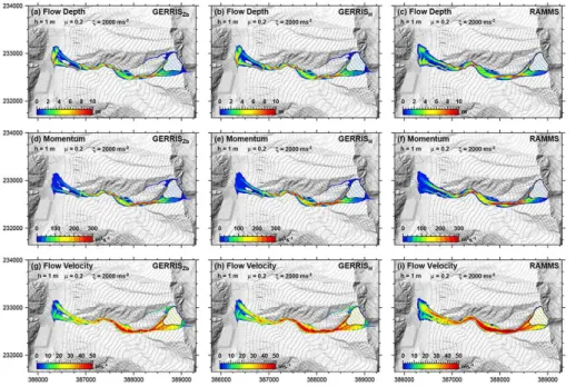
route the granular fluid to the nearly flat valley floor representing the runout zone of the avalanche (Fig. 8).

We compare the maximum values (at each point, taken over the entire simulation) of flow depth, momentum, and velocity of the modeled avalanche. Momentum is defined as the product of flow depth and velocity in this context. We set the release height

5

to h₌1 m and define spatially constant parameters for the Voellmy flow resistance

law (µ₌0.2,ξ₌2000 m s−2). Generally, the deviations between GERRIS_Zb, GERRIS_H, and RAMMS are small, and the first-order features of the avalanche agree well between the two GERRIS approaches and RAMMS. This includes flow depths, runout distances, flow velocities, and momentum.

10

However, a closer examination reveals some second-order deviations between the

different numerical approaches. RAMMS shows a more pronounced tendency to

over-flow counter hillsides and to keep the over-flow direction even uphill. This is clearly doc-umented at the lower third of the avalanche track where the avalanche is split into two branches. Here the orographic right flow path is characterized by a considerable

15

uphill section. In this domain, the results of RAMMS show higher values in the maxi-mum flow depth compared to the two GERRIS approaches (Fig. 8a–c). The modeled avalanches in RAMMS overflow larger areas causing a wider flow path than predicted by the GERRIS experiments. This is recognized most clearly in the S-shaped gully section. A broader flow path and the tendency to flow uphill observed in avalanches

20

modeled with RAMMS relative to those modeled with GERRISZb and GERRISH are

caused by larger values in the momentum (Fig. 8d–f) arising from slightly higher flow velocities especially in the gully section of the thalweg (Fig. 8g–i).

In contrast to the small deviations found in the previous examples, this effect is a di-rect consequence of applying only cordi-rections to the longitudinal acceleration. When

25

(20)

NHESSD

2, 6775–6809, 2014

Title Page

Tables Figures

◭ ◮

Back Close

Full Screen / Esc

Discussion

P

a

per

|

Discus

sion

P

a

per

|

Discussion

P

a

per

|

Discussion

P

a

per

|

corrected, so that the tendency of the avalanche to stay within the gully is stronger than in RAMMS.

A further deviation is observed in the runout zone where the shapes of the avalanche

deposit of the RAMMS simulations differ considerably from those of the GERRIS

sim-ulations, while the runout distances and base areas of the avalanche deposits of the

5

three models agree well. The discrepancy in the shape of the deposits is similar to that found when considering the runout on the simple concave topography in Sect. 4.2,

and it is presumably related to the different numerical schemes used in RAMMS and

GERRIS rather than to our approximations. Beyond this, the shape of the deposits

may slightly differ because the RAMMS simulations terminate by default when the

mo-10

mentum of the fluid drops below 5 % of the maximum momentum, while the GERRIS

simulations were defined to terminate att₌240 s.

Finally, the differences between the realizations GERRISHwhere the corrections in

the friction term are based an the fluid surface and GERRIS_Zbwhere the corrections are computed from the original topography are very small in this example. So the stronger

15

(although not serious) artefacts occurring at the avalanche front in GERRISH(Sect. 4.1)

and the higher stability of GERRIS_Zbat the transition to the tail remain the only

notice-able difference between both GERRIS-based approaches. These differences suggest

that using the version GERRISZbmay in general be preferable to GERRISH.

5 Conclusions

20

The examples considered in Sect. 4 show that granular avalanches can be simulated using the shallow water equations directly in Cartesian coordinates even in steep ter-rain if an appropriate additional friction term is included. This finding allows the utiliza-tion of software that was originally designed for other purposes, namely modeling the flow of water in rivers, lakes, and oceans.

25

(21)

NHESSD

2, 6775–6809, 2014

Title Page

Tables Figures

◭ ◮

Back Close

Full Screen / Esc

Discussion

P

a

per

|

Discus

sion

P

a

per

|

Discussion

P

a

per

|

Discussion

P

a

per

|

adjustable for this purpose is available. Some of them are even freely available. There-fore, research on avalanches can easily profit from the enormous effort that has already been spent in developing numerical codes in fluid dynamics. The implementations pre-sented in this paper are based on the software GERRIS, but this shall only be seen as an example. Apart from begin freely available and providing state-of-the-art numerics,

5

GERRIS allows the implementation of our method with a moderate effort. However, this

shall not imply that GERRIS is indeed the best software for this purpose.

The examples investigated for validation have only revealed minor deviations towards the commercial model RAMMS used as a reference, in particular with regard to the properties of avalanches relevant for hazard assessment. For the artificial, basically

10

one-dimensional geometries investigated in Sects. 4.1 and 4.2, the agreement between our implementations based on GERRIS and RAMMS is even excellent. The small dif-ferences between the approaches encountered here are probably not related to the

approximations introduced in our theory, but arise from di_fferent numerical schemes

used for solving the equations of motion. So the approach presented in this study can

15

fully compete with commercial software for mass movements flowing on open flanks or if large volumes and high flow depths occur and small gullies do not influence the flow characteristics strongly. For such geometries the deviations between result of our

ap-proach from those of RAMMS are far offfrom having any implications on the mitigation

strategy based on predicted properties of the modeled avalanche.

20

The example based on a complex topography (Sect. 4.3) reveals still rather small, but

perhaps not always negligible differences between our approach and RAMMS. RAMMS

solutions show larger flow depths in avalanche tracks with prominent uphill sections and expanded overflowed areas in steep, twisted gullies. In contrast to the differences discussed above, these deviations arise from the approximations discussed in Sect. 3

25

(22)

NHESSD

2, 6775–6809, 2014

Title Page

Tables Figures

◭ ◮

Back Close

Full Screen / Esc

Discussion

P

a

per

|

Discus

sion

P

a

per

|

Discussion

P

a

per

|

Discussion

P

a

per

|

However, when discussing differences between models on such a small level we

should keep in mind that all these modeling approaches involve a considerable inher-ent uncertainty compared to other flow processes such as the flow of water in lakes and oceans. These uncertainties start with the basic assumption of the granular medium as a single layer continuum and the rheology (e.g. Voellmy’s friction law). It continues

5

with the determination of the relevant parameters for dry snow avalanches and does not stop at the determination of the release zone in form of spatial position, extent, and involved volumes (fracture depth). Even the resolution and quality of the applied digi-tal elevation model can highly influence the avalanche path (Bühler et al., 2011), and taking into account further processes such as entrainment introduces an additional

un-10

certainty in the parameters. Assessing these uncertainties quantitatively goes beyond the scope of this paper, but in sum, they are obviously larger than the small deviations between the models.

The di_fferences between the two proposed implementations based on GERRIS are

also small. The version GERRISZb where the correction terms are computed from the

15

original topography is less prone to artefacts at the avalanche front and at the transition to the tail than the version GERRIS_Husing the fluid surface, without revealing significant drawbacks anywhere. We therefore suggest to compute the friction terms from the topographic slope instead of the fluid surface.

Although our validation focused on snow avalanches, the approach is in principle

20

also applicable to other rapid mass movements such as debris flows. Debris flows are characterized by lower flow velocities and lower flow path gradients compared to snow

avalanches, so that e_ffects of our approximations become even less significant.

Be-side of model set-ups with a pre-defined release volume, a huge number of scenarios

involving different release zones characterized by discharge-time series can be

eas-25

ily implemented within the GERRIS parameter file. In principle the initiation of surface

runoffcan be defined at each mesh element, so that flooding and debris flow

simula-tions based on precipitation time series for storm events are possible without preceding

(23)

NHESSD

2, 6775–6809, 2014

Title Page

Tables Figures

◭ ◮

Back Close

Full Screen / Esc

Discussion

P

a

per

|

Discus

sion

P

a

per

|

Discussion

P

a

per

|

Discussion

P

a

per

|

defined in the parameter file, so that the implementation of other rheological models (e.g. Bingham fluid) is straightforward and requires no specific coding skills.

We propose that our approach based on GERRIS is suitable for regional scale dense snow avalanche studies on complex terrain and probably also for other types of rapid mass movements. However, dimensioning of permanent protection measures requires

5

numerical models that have been calibrated by the backward analysis of numerous monitored real world avalanches as, for example, performed by the SLF at the Vallèe de la Sionne. In principle, the parameters of the Voellmy fluid model calibrated for RAMMS are fully compatible with our approach, and spatially variable parameter values can be easily implemented in the GERRIS parameter file. This also applies to extensions of

10

the flow law such as the cohesion term implemented in the recent version of RAMMS. Thus, a more or less complete compatibility with RAMMS can be achieved. However, as we did not perform backward analysis calculations to calibrate the fluid model for our approach on our own and tested the compatibility only for a few examples, the modeling results should be taken with caution when mitigation strategies and protection

15

measures are developed. For such applications, the compatibility with established and extensively tested software packages should be ascertained for the given conditions, or at least a careful backward analysis of the specific avalanche should be conducted.

Appendix A: Implementation in GERRIS

The following lines of code show the implementation of our approach in the GERRIS

20

(24)

NHESSD

2, 6775–6809, 2014

Title Page

Tables Figures

◭ ◮

Back Close

Full Screen / Esc

Discussion

P

a

per

|

Discus

sion

P

a

per

|

Discussion

P

a

per

|

Discussion

P

a

per

|

# Gradient of the original topography (GERRIS_Zb)

# For version GERRISHreplace “Zb” with “H”

DX = dx("Zb") DY = dy("Zb")

# tan2ϕaccording to Eq. (3)

TAN2PHI = DX*DX+DY*DY

# sin2ϕfrom basic trigonometric relations

SIN2PHI = TAN2PHI/(1.+TAN2PHI)

# cosϕfrom basic trigonometric relations

COSPHI = 1./sqrt(1+TAN2PHI)

# tanψ according to Eq. (4)

TANPSI = -(DX*U+DY*V)/sqrt(U*U+V*V+eps)

# cosψ from basic trigonometric relations

COSPSI = 1./SQRT(1+TANPSI*TANPSI)

# Factor ₁₊1_δtf occurring in Eq. (19) withf according to Eq. (16).

F = (P > DRY ? Velocity/(Velocity+dt*GRAV*(SIN2PHI*TANPSI+ mu*COSPHI*COSPSI+Velocity*Velocity/(P*Xi*COSPHI*COSPSI))): 0.)

# Multiply both components of the velocity byF according to Eq. (19)

U = U*F V = V*F

# Magnitude of the 3-dimensioal velocity vector

Vtotal = (P > DRY ? Velocity/COSPSI: 0)

# Flow depth normal to the topography

localDepth = P * COSPHI

(25)

NHESSD

2, 6775–6809, 2014

Title Page

Tables Figures

◭ ◮

Back Close

Full Screen / Esc

Discussion

P

a

per

|

Discus

sion

P

a

per

|

Discussion

P

a

per

|

Discussion

P

a

per

|

Acknowledgements. We thank ILF Consulting Engineers for licensing RAMMS in the course

of a common project and the federal government of Salzburg for implementing the INSPIRE guidelines and providing ALS digital elevation models with a resolution of 10 m.

References

An, H. and Yu, S.: Well-balanced shallow water flow simulation on quadtree cut cell grids, Adv.

5

Water Resour., 39, 60–70, doi:10.1016/j.advwatres.2012.01.003, 2012. 6778

Berger, M. J., George, D. L., LeVeque, R. J., and Mandli, K. T.: The GeoClaw software for depth-averaged flows with adaptive refinement, Adv. Water Resour., 34, 1195–1206, doi:10.1016/j.advwatres.2011.02.016, 2011. 6778

Bühler, Y., Christen, M., Kowalski, J., and Bartelt, P.: Sensitivity of snow avalanche

sim-10

ulations to digital elevation model quality and resolution, Ann. Glaciol., 52, 72–80, doi:10.3189/172756411797252121, 2011. 6796

Christen, M., Kowalski, J., and Bartelt, P.: RAMMS: Numerical simulation of dense snow avalanches in three-dimensional terrain, Cold Reg. Sci. Technol., 63, 1–14, doi:10.1016/j.coldregions.2010.04.005, 2010. 6777, 6779, 6785

15

Fischer, J.-T., Kowalski, J., and Pudasaini, S. P.: Topographic curvature ef-fects in applied avalanche modeling, Cold Reg. Sci. Technol., 74–75, 21–30, doi:10.1016/j.coldregions.2012.01.005, 2012. 6779, 6785, 6789

Granig, M. and Jörg, P.: A dynamic aproach to evaluate the dense and powder snow avalanche model SAMOS-AT, in: 12th Congress Interpraevent, 23–26 April 2012, Grenoble, France,

20

Extended Abstracts, edited by: Koboltschnig, G., Hübl, J., and Braun, J., 196–197, 2012. 6777

Horton, P., Jaboyedoff, M., Rudaz, B., and Zimmermann, M.: Flow-R, a model for susceptibility mapping of debris flows and other gravitational hazards at a regional scale, Nat. Hazards Earth Syst. Sci., 13, 869–885, doi:10.5194/nhess-13-869-2013, 2013. 6777

25

(26)

NHESSD

2, 6775–6809, 2014

Title Page

Tables Figures

◭ ◮

Back Close

Full Screen / Esc

Discussion

P

a

per

|

Discus

sion

P

a

per

|

Discussion

P

a

per

|

Discussion

P

a

per

|

Keiler, M., Sailer, R., Jörg, P., Weber, C., Fuchs, S., Zischg, A., and Sauermoser, S.: Avalanche risk assessment – a multi-temporal approach, results from Galtür, Austria, Nat. Hazards Earth Syst. Sci., 6, 637–651, doi:10.5194/nhess-6-637-2006, 2006. 6777

Kirschbaum, D. B., Adler, R., Hong, Y., Hill, S., and Lerner-Lam, A.: A global landslide cat-alog for hazard applications: method, results, and limitations, Nat. Hazards, 52, 561–575,

5

doi:10.1007/s11069-009-9401-4, 2010. 6776

LeVeque, R. J., George, D. L., and Berger, M. J.: Adaptive mesh refinement techniques for tsunamis and other geophysical flows over topography, Acta Numer., 20, 211–289, doi:10.1017/S0962492911000043, 2011. 6778

Medina, V., Hürlimann, M., and Bateman, A.: Application of FLATModel, a 2D finite volume

10

code, to debris flows in the northeastern part of the Iberian Peninsula, Landslides, 5, 127– 142, doi:10.1007/s10346-007-0102-3, 2008. 6777

Mergili, M., Schratz, K., Ostermann, A., and Fellin, W.: Physically-based modelling of granular flows with Open Source GIS, Nat. Hazards Earth Syst. Sci., 12, 187–200, doi:10.5194/nhess-12-187-2012, 2012. 6779

15

Popinet, S.: An accurate adaptive solver for surface-tension-driven interfacial flows, J. Comput. Phys., 228, 5838–5866, doi:10.1016/j.jcp.2009.04.042, 2009. 6778

Popinet, S.: Adaptive modelling of long-distance wave propagation and fine-scale flooding dur-ing the Tohoku tsunami, Nat. Hazards Earth Syst. Sci., 12, 1213–1227, doi:10.5194/nhess-12-1213-2012, 2012. 6778

20

Pudasaini, S. P. and Hutter, K.: Rapid shear flows of dry granular masses down curved and twisted channels, J. Fluid Mech., 495, 193–208, doi:10.1017/S0022112003006141, 2003. 6779

Sailer, R., Fellin, W., Fromm, R., Jörg, P., Rammer, L., Sampl, P., and Schaffhauser, A.: Snow avalanche mass-balance calculation and simulation-model verification, Ann. Glaciol., 48,

25

183–192, doi:10.3189/172756408784700707, 2008. 6777

Sampl, P. and Zwinger, T.: Avalanche simulation with SAMOS, Ann. Glaciol., 38, 393–398, doi:10.3189/172756404781814780, 2004. 6777

Sheridan, M. F., Stinton, A. J., Patra, A., Pitman, E. B., Bauer, A., and Nichita, C. C.: Evaluating Titan2D mass-flow model using the 1963 Little Tahoma Peak avalanches, Mount Rainier,

30

(27)

NHESSD

2, 6775–6809, 2014

Title Page

Tables Figures

◭ ◮

Back Close

Full Screen / Esc

Discussion

P

a

per

|

Discus

sion

P

a

per

|

Discussion

P

a

per

|

Discussion

P

a

per

|

Voellmy, A.: Über die Zerstörungskraft von Lawinen, Schweiz. Bauzeitung, 73, 159–165, 212– 217, 246–249, 280–285, 1955. 6777, 6782

Weller, H. and Weller, H. G.: A high-order arbitrarily unstructured finite-volume model of the global atmosphere: tests solving the shallow-water equations, Int. J. Numer. Fl., 56, 1589– 1596, doi:10.1002/fld.1595, 2008. 6778

(28)

NHESSD

2, 6775–6809, 2014

Title Page

Tables Figures

◭ ◮

Back Close

Full Screen / Esc

Discussion

P

a

per

|

Discus

sion

P

a

per

|

Discussion

P

a

per

|

Discussion

P

a

per

|

Figure 1.Different coordinate systems used for modeling mass movements in a channel not

(29)

NHESSD

2, 6775–6809, 2014

Title Page

Tables Figures

◭ ◮

Back Close

Full Screen / Esc

Discussion

P

a

per

|

Discus

sion

P

a

per

|

Discussion

P

a

per

|

Discussion

P

a

per

|

(b) Avalanche Profile at t = 20 s

ϕ = 30° µ = 0.2 _ξ_{= 1000 ms}-2

0 5 10 15

Velocity [ms

-1]

x [m] 0.0 0.5 1.0 1.5 2.0

Flow Depth [m]

GERRISH

GERRISZb

RAMMS

-500 -750

-1000 -250

Terminal Velocity

-550

-500

-450

-400

-350

-300

-250

-200

-150

-100

-50

0

50

100

150

200

250

300

350

400

450

500

550

(a) GERRISH - Flow Depth at t = 20 s

ϕ = 30°

µ = 0.2 ξ = 1000 ms-2

m -500

-250 0 250

y [m]

-1000 -750 -500 -250 0 250 500 750 x [m]

0 1 2 3

m

Figure 2.Comparison of two different numerical solutions of GERRIS with RAMMS for granular

(30)

NHESSD

2, 6775–6809, 2014

Title Page

Tables Figures

◭ ◮

Back Close

Full Screen / Esc

Discussion

P

a

per

|

Discus

sion

P

a

per

|

Discussion

P

a

per

|

Discussion

P

a

per

|

Figure 3.Test of the numerical results of GERRIS_Zb(symbols) against the one-dimensional

an-alytical time dependent solution for a Voellmy fluid flowing on a flow path with a constant slope (Eq. 25, solid lines) for several parameter sets for(a)flow depthh,(b)turbulence parameterξ,

(31)

NHESSD

2, 6775–6809, 2014

Title Page

Tables Figures

◭ ◮

Back Close

Full Screen / Esc

Discussion

P

a

per

|

Discus

sion

P

a

per

|

Discussion

P

a

per

|

Discussion

P

a

per

|

Figure 4.Two-dimensional representation of numerical solutions of GERRIS_Zb for flow depth

and flow velocity of a partly concave slope at four different time steps. The fluid layer accelerates at an inclined ramp (ϕ₁=30◦) and runs out in a gently dipping surface (ϕ₂=5◦) with a smooth transition. A topographic profile of the geometry is shown in the inset of(a). The white dashed-dotted line indicates the position of the longitudinal profiles shown in Figs. 5 and 6.