David Greenlaw, Morgan Stanley
Jan Hatzius,Goldman Sachs
Anil K Kashyap,University of Chicago Graduate School of Business
Hyun Song Shin,Princeton University
. . . .
.. .. ... .. .. ... .. .. ... .. .. ... .. .. ...
Proceedings of the U.S. Monetary Policy Forum 2008
changed the nature of business in the 21st Century. They have also generated confusion among policymakers and the public.
Chicago Graduate School of Business (GSB) will continue our role as thought leader on how these markets work, their effects, and the way they interact with policies and institutions.
The Initiative on Global Markets will organize our efforts. It will support original research by Chicago GSB faculty, prepare our students to make good decisions in a rapidly changing business environment, and exchange ideas with policymakers and leading international companies about the biggest issues facing the global economy.
The Initiative will span three broad areas:
■International business
■Financial markets
■The role of policies and institutions
By enhancing the understanding of business and financial market globalization, and by preparing MBA students to thrive in a global environment, the initiative will help improve financial and economic decision-making around the world.
The Initiative on Global Markets was launched with a founding grant from the Chicago Mercantile Exchange (CME) Trust and receives ongoing financial support from the CME Trust and our corporate partners: AQR Capital Management, Barclays Bank PLC, John Deere, and Northern Trust Corporation.
is Brandeis International Business School’s principal research platform in the field of international finance. The Institute seeks to analyze and anticipate major trends in global financial markets, institutions, and regulations, and to develop the information and ideas required to solve emerging problems. To this end, the Institute promotes informal exchanges among scholars and practitioners, research, and policy analyses, and also participates in the School’s teaching programs.
The Institute is named in honor of Dr. Barbara Rosenberg ‘54, a prominent educator and alumna of Brandeis University, and Mr. Richard M. Rosenberg, the former Chairman and CEO of Bank of America.
The Institute addresses a key issue in international finance each year by commissioning research studies from faculty members at Brandeis and other institutions, by scheduling talks by visiting experts, by offering new courses, and by organizing a major annual conference. The Institute is committed to connecting IBS’s and other academic research with the insights of business and policy leaders, and to use research to inform major global business and policy decisions.
Foreword . . . .5 Acknowledgements . . . .6 U
U..SS.. MMoonneettaarryy PPoolliiccyy FFoorruumm 22000088 RReeppoorrtt:: . . . .7 L
Leevveerraaggeedd LLoosssseess:: LLeessssoonnss ffrroomm tthhee MMoorrttggaaggee MMaarrkkeett MMeellttddoowwnn
Abstract . . . .8 Comments by Frederic S. Mishkin . . . .60 Member of the Board of Governors of the Federal Reserve System
Comments by Eric S. Rosengren . . . .67 President and CEO of the Federal Reserve Bank of Boston
Luncheon Address: Vincent Reinhart . . . .7 Resident Scholar, The American Enterprise Institute
The Governance, Communication, and Conduct of the Federal Reserve’s Monetary Policy
P
Prroocceeeeddiinnggss ooff tthhee RRoouunnddttaabbllee DDiissccuussssiioonn . . . .87 o
onn ““BBaallaanncciinngg FFiinnaanncciiaall SSttaabbiilliittyy,, PPrriiccee SSttaabbiilliittyy,, aanndd M
Maaccrrooeeccoonnoommiicc SSttaabbiilliittyy:: HHooww IImmppoorrttaanntt iiss MMoorraall HHaazzaarrdd??””
Comments by Charles L. Evans . . . .88 President and CEO of the Federal Reserve Bank of Chicago
Comments by Peter Hooper . . . .91 Managing Director and Chief Economist, Deutsche Bank Securities
Comments by William Poole . . . .95 President and CEO of the Federal Reserve Bank of St. Louis
Comments by Kenneth D. West . . . .100 Ragnar Frisch Professor of Economics and Chair of the Economics Department
University of Wisconsin-Madison
Author Biographies . . . .103 U.S. Monetary Policy Forum 2008 List of Participants . . . .111
. . .
Foreword
The U.S. Monetary Policy Forum (USMPF) is an annual conference that brings academics, market economists, and policymakers together to discuss U.S. monetary policy. A standing group of academic and private sector economists (the USMPF panelists) has rotating responsibility for producing a report on a critical medium-term issue confronting the Federal Open Market Committee (FOMC).
The 2008 USMPF panel includes private-sector members David Greenlaw (Morgan Stanley), Jan Hatzius (Goldman Sachs), Ethan Harris (Lehman), Peter Hooper (Deutsche Bank), Bruce Kasman (JP Morgan Chase), and Kim Schoenholtz (Citigroup), as well as academic panelists Stephen Cecchetti (Brandeis), Anil Kashyap (Chicago), Matthew Shapiro (Michigan), Hyun Song Shin (Princeton), and Mark Watson (Princeton).
This volume reports the results of the second USMPF conference, held on February 29, 2008 in New York, N.Y. The meeting, attended by over 100 central bankers, academics, business economists, and journalists, began with a presentation of this year’s report, followed by a luncheon address delivered by former FOMC Secretary Vincent Reinhart, and ended with a panel discussion.
The second USMPF report, Leveraged Losses: Lessons from the Mortgage Market Meltdown, authored by Greenlaw, Hatzius, Kashyap, and Shin focuses on lessons from the credit crisis for central banking. Following the authors’ presentation, Federal Reserve Board Governor Frederic Mishkin, and Eric Rosengren, President, Federal Reserve Bank of Boston, offered their comments.
This year’s policy panel was entitled “Balancing Financial Stability, Price Stability, and Macroeconomic Stability: How Important is Moral Hazard?” The discussion featured presentations by Charles Evans and William Poole, Presidents of the Federal Reserve Banks of Chicago and St. Louis, respectively, as well as by panel members Hooper and West.
The USMPF is sponsored jointly by the Initiative on Global Markets at the University of Chicago Graduate School of Business and the Rosenberg Institute for Global Finance at the Brandeis International Business School.
Stephen G. Cecchetti and Anil K Kashyap, Co-Directors Waltham, Massachusetts and Chicago, Illinois, June 2008
Acknowledgements
The U.S. Monetary Policy Forum acknowledges the generous financial support of the Rosenburg Institute for Global Finance and the corporate partners of the Initiative on Global markets: AQR Capital Management, Barclays, Chicago Mercantile Exchange Trust, John Deere, and Northern Trust. We also wish to thank Goldman Sachs and Morgan Stanley for providing their support.
In addition to institutional support, there were a number of people whose help was essential to our success. First, there are all of the members of the USMPF panel, who offered comments and encouragement. Second, we thank the FOMC members, who attended the meeting and spoke on the record. We extend a special thanks to William Dudley, System Open Market Manager, Jeffrey Lacker, Charles Plosser, and Gary Stern, the Presidents of the Federal Reserve Banks of Richmond, Philadelphia, and Minneapolis respectively, who accepted our invitation to attend the meeting. Finally, there were several people behind the scenes who deserve special mention. These include Allan Friedman and Janice Luce of the University of Chicago Graduate School of Business and Matthew Parillo at the Brandeis International Business School. We owe a special thanks to Jennifer Williams for organizing the conference and overseeing all the conference operations.
David Greenlaw, Jan Hatzius, Anil K Kashyap, Hyun Song Shin
U.S. Monetary Policy Forum Report No. 2,
Rosenberg Institute, Brandeis International Business School and
Initiative on Global Markets, University of Chicago Graduate School of Business, 2008
. . .
LEVERAGED LOSSES:
Lessons from the Mortgage Market Meltdown
** Affiliations are Greenlaw (Morgan Stanley), Hatzius (Goldman Sachs), Kashyap (University of Chicago GSB, National Bureau of Economic Research, and Federal Reserve Bank of Chicago), and Shin (Princeton). We thank the USMPF panelists, Tobias Adrian, and Raghuram Rajan for helpful comments and suggestions. We thank Biliana Kassabova, Yian Liu, and Shirla Sum for outstanding research assistance. We also thank Tim Grunwald, Vishwanath Tirupattur and Andrew Sheets for supplying data. Finally, we thank Patrick Oliver for editorial assistance. The views expressed here are those of the authors only and not necessarily of the institutions with which they are affiliated. All errors are our own.
©2008U.S. Monetary Policy Forum
LEVERAGED LOSSES:
Lessons from the Mortgage Market Meltdown
by
David Greenlaw, Jan Hatzius,
Anil K Kashyap, Hyun Song Shin
Abstract
This report discusses the implications of the recent financial market turmoil for central banks. We start by characterizing the disruptions in the financial markets and compare these dislocations to previous periods of financial stress. We confirm the conventional view that the current problems in financial markets are concentrated in institutions that have exposure to mortgage securities. We use several methods to estimate the ultimate losses on these securities. Our best (very uncertain) guess is that the losses will total about $500 billion, with about half being borne by leveraged U.S. financial institutions. We then highlight the role of leverage and mark-to-market accounting in propagating this shock. This perspective implies an estimate of the eventual contraction in balance sheets of these institutions, which will include a substantial reduction in credit to businesses and households. We close by exploring the feedback from credit availability to the broader economy and provide new evidence that contractions in financial institutions’ balance sheets cause a reduction in real GDP growth.
1. Introduction
This report seeks to characterize and explain the credit market turmoil that began to grab headlines in August 2007. The associated fall-out has been an important driver of central bank policies since that time. Indeed, a number of Fed officials have linked these
developments to monetary policy actions taken over the course of the past several months (see Bernanke [2007a,b and 2008], Evans [2007], Kroszner [2007], Mishkin [2007a,b], Poole [2007], and Rosengren [2007a,b]). This report offers a theory as to why credit market disruptions matter for the macro economy and some estimates of what the turmoil might imply about future growth.
Our analysis is broken down into four parts. We begin, in section 2, with a description of the key credit market events since August 2007. In doing so, we demonstrate that the credit crisis was not an across-the-board deterioration of all credit markets, but — at least in its early stages — an acute crisis that affected certain markets while leaving others virtually unscathed. At the epicenter of the turmoil are mortgage-related securities.
Having established the central role of mortgage-related debt in the crisis, in section 3, we try to assess the size of these credit losses and where those losses are concentrated. We find that the brunt of the losses are borne by the financial intermediary sector – both the traditional banks and broker dealers, as well as other entities involved in the
securitization process.
In section 4, we offer an argument as to why the incidence of the losses (i.e., who bears the losses) is as important as how large those losses are. The characteristic feature of the financial intermediary sector is that it is composed of leveraged institutions whose capital is a small proportion of the total assets they hold. Credit losses deplete their capital cushion. We show that in past episodes, when faced with capital losses, intermediaries have scaled back their leverage and tried to rebuild their capital. Consequently, the overall decline in lending following the losses depends not only on the size of the initial shock, but also on the ability to raise new capital and on the extent to which the
intermediaries reduce their target level of leverage. We provide a range of possible adjustments, but as a rule the overall lending reduction is many times larger than the capital losses. Our baseline estimates imply a $2.3 trillion contraction in intermediary balance sheets, of which roughly $1 trillion would represent a decline in lending to households, businesses, and other non-levered entities.
This impending reduction in lending provides a possible link between the initial problems in the mortgage market and the rest of the economy. In section 5, we explore this channel. We first confirm past findings that have shown growth in total business credit to be
they still suggest that the feedback from the financial market turmoil to the real economy could be substantial.
We conclude with some provisional lessons for central banks from the events thus far.
2. Credit Market Developments Since August 2007
We begin by describing the main events in the credit market since August 2007. In doing so, we note that some markets did not initially show signs of stress, which we will argue in the rest of the report helps pinpoint the transmission channels operating during this crisis.
2.1 The markets that were disrupted
Signs of severe pressures in some credit markets became evident across the globe on August 9. In an interesting geographic twist, the proximate trigger seemed to be the announcement by a large European bank that it would close three investment funds because problems in the U.S. mortgage market had made it impossible to value the underlying assets.
Exhibit 2.1 LIBOR Rate
In response to emerging signs of stress, the overnight London Interbank Offer Rate
(LIBOR) set more than 50 basis points (bp) higher than the previous day (see Exhibit 2.1). Term interbank funding rates — a measure that we will return to throughout this study
— showed a similar move. LIBOR is a key benchmark rate for many types of consumer and business loans. Indeed, data compiled by the Federal Reserve Bank of New York (2007) indicate that 6-month LIBOR serves as the index rate for virtually all subprime
2.0 2.5 3.0 3.5 4.0 4.5 5.0 5.5 6.0
Jan FebMar Apr May Jun Jul Aug Sep Oct Nov Dec Jan Feb Mar Apr May 2.0 2.5 3.0 3.5 4.0 4.5 5.0 5.5 6.0
Overnight 1-Month 3-Month
Percent Percent
2007 2008
London Interbank Offered Rate:
mortgage loans outstanding in the U.S. As we will demonstrate, the move in LIBOR on August 9 and the days immediately following was particularly noteworthy given evolving market expectations of future Fed rate cuts.
Meanwhile, the ECB — citing “tensions in the euro money market” — injected more than $130 billion into the system on August 9 in the type of emergency operation that had not been conducted since the aftermath of the September 2001 terrorist attacks. The Federal Reserve followed with unusually aggressive open market operations of its own a few hours later. Just days earlier, the Federal Open Market Committee (FOMC) had decided to leave monetary policy unchanged and had issued a statement that indicated the predominant policy concern was tilted toward inflation risk. But, on August 17, as signs of tightening credit conditions became increasingly apparent, the FOMC formally altered its assessment of the risks confronting the economy, and the Board of Governors slashed the discount rate by 50 bp.
The events that began to play out on August 9 triggered an intense examination of investor exposure to risk in the U.S. mortgage market. In the next section of this report, we assess the magnitude of losses tied to subprime mortgages, but it’s clear that one of the reasons that problems in this sector began to have far-reaching effects is that the loans under scrutiny were embedded in a wide variety of securities. Moreover, financial
intermediaries had exposure to both the securities and the underlying loans. Thus, not only did the elevated risk now apparent in the subprime mortgage market lead to a sharp slowdown in origination of such loans, but there was significant spillover to other sectors such as jumbo mortgages, asset-backed commercial paper, and collateralized debt
obligations (CDO’s).
Exhibit 2.2 Jumbo Mortgage Spread
0 20 40 60 80 100 120 140 160 180
98 99 00 01 02 03 04 05 06 07
0 20 40 60 80 100 120 140 160 180 Jumbo Mortgage Spread
Basis points Basis points
Jumbo mortgages account for 17% of the dollar value of all first-lien mortgage debt outstanding in the U.S., with nearly half of the loans being securitized. Roughly 50% of all jumbo mortgages are tied to homes located in the state of California (Office of Federal Housing Enterprise Oversight [2008]). Exhibit 2.2 shows a spike in the spread between jumbo and conforming mortgage rates that appeared first in August 2007. The typical spread is in the range of 20bp to 40bp, but since mid-August it has been much higher.
Exhibit 2.3 Asset-Backed Commercial Paper (ABCP) Yields
2.0 2.5 3.0 3.5 4.0 4.5 5.0 5.5 6.0 6.5
Jan Feb Mar Apr May Jun Jul Aug Sep Oct Nov Dec Jan Feb Mar Apr May 2.0 2.5 3.0 3.5 4.0 4.5 5.0 5.5 6.0 6.5
Overnight 1 Month
Asset-Backed Commercial Paper Yields: Percent
Source: Federal Reserve Board
Percent
2007 2008
Exhibit 2.4 Commercial Paper Outstanding
0 500 1000 1500 2000 2500
2001 2002 2003 2004 2005 2006 2007 2008
0 500 1000 1500 2000 2500
Total
Commerical Paper Outstanding: Billions of dollars
Source: Federal Reserve Board
Billions of dollars
Similarly, rates on asset-backed commercial paper spiked in mid-August (see Exhibit 2.3). Asset-backed Commercial Paper (ABCP) is a security issued by a bank or other financial entity with a maturity that is typically between 1 and 180 days. The notes are backed by the physical assets that are used as collateral for loans to households or businesses. The asset-backed component of the commercial paper (CP) market had grown at a
phenomenal clip in recent years, and at the start of August it accounted for more than one-half of the $2.2 trillion of all CP outstanding (see Exhibit 2.4). According to a speech by William Dudley of the Federal Reserve Bank of New York, data from Moody’s show that only about 25% of the collateral underlying ABCP as of mid-2007 consisted of residential mortgages (Dudley [2007]). However, while the direct exposure to subprime mortgage debt was relatively limited and the majority of ABCP programs were highly rated, investors appeared to have a great deal of difficulty evaluating the credit quality of the underlying assets. Issuers were confronted with an inability to roll maturing paper. Such a development would likely lead to either a forced liquidation of the underlying assets or the triggering of backstop credit agreements that would bring the assets onto bank balance sheets and intensify the strains that were already evident in term funding markets.
Exhibit 2.5 Senior Loan Officer Survey
-60 -40 -20 0 20 40 60 80
90 92 94 96 98 00 02 04 06 08
-60 -40 -20 0 20 40 60 80
Mortgage Credit Cards
Prime Mortgages Subprime Mortgages
Commercial & Industrial Percent
Net Percentage of Banks Reporting Tightening of Standards:
Percent
Source: Federal Reserve Board
the share of credit intermediation by depository institutions and by the securities markets. Examples of the former include mortgages, C&I loans, and credit card debt that remains on balance sheet. Examples of the latter include corporate bonds, commercial paper, and asset-backed securities. Note that the shares do not add up to 100% because a small amount of intermediation occurs in a direct fashion — such as when a pension fund provides financing for a commercial mortgage. The securities market is certainly the dominant source of intermediation in the U.S. today. This is one of the ways in which the latest episode of credit tightening differs from those experienced in the 1980s and earlier. However, while the banking sector currently plays a much smaller role in the
intermediation process than it did a couple of decades ago, it can still serve as an important allocator of credit and provider of liquidity in times of stress.2
Exhibit 2.6 Share of Intermediation through Banks and Securities Markets
25 30 35 40 45 50 55 60
80 83 86 89 92 95 98 01 04 07
25 30 35 40 45 50 55 60
Intermediated Through Securities Markets Intermediated Through Depository Institutions Percent
Share of Private Nonfinancial Debt Outstanding:
Source: Morgan Stanley calculations based on Federal Reserve Flow of Funds Accounts
Percent
2.2 Other non-affected markets
We now turn to another important characteristic of recent financial market developments
— the delayed spillover effects. In the midst of the considerable pressures that we have described during the early stages of the credit tightening, some important asset classes seemed little affected. Indeed, even relatively high-risk assets appeared to be immune to the initial signs of stress in the banking sector, mortgage market, and commercial paper market. Exhibit 2.7 shows monthly total returns for a variety of asset classes starting in July 2007. While most assets classes had negative returns in July, the cumulative returns
2
from July through October for all of the domestic indices, except the S&P financials, were positive. Only in November did clear signs of stress begin to appear.
Exhibit 2.7 Monthly Total Returns on Various Asset Classes, July 2007 to January 2008
Jul-07 Aug-07 Sep-07 Oct-07 Nov-07 Dec-07 Jan-08
S&P 500 -3.1% 1.5% 3.7% 1.6% -4.2% -0.7% -6.0%
S&P Financials -7.8% 1.5% 2.3% -1.8% -7.7% -5.4% -0.3%
Nasdaq -2.2% 2.0% 4.0% 5.8% -6.9% -0.3% -9.9%
Ryan Labs US Treasuries 1.8% 2.3% -0.2% 2.8% 2.9% -0.6% 3.7%
Merrill Lynch High Grade Corporate Bonds 0.6% 1.0% 0.5% 0.7% 1.4% 0.3% 2.2%
Merrill Lynch High Yield Bonds -3.1% 1.1% 2.4% 0.6% -2.0% 0.3% -1.4%
EMBI+ -0.9% 1.6% 2.4% 2.6% -0.5% 0.6% 0.7%
MSCI Europe (Local) -3.5% -0.5% 1.7% 2.9% -3.8% -0.5% -11.4%
MSCI EAFE (Local) -3.2% -1.4% 2.3% 2.4% -4.1% -1.2% -10.9%
MSCI EM (Local) 4.9% -0.9% 8.4% 9.0% -6.2% 0.6% -12.4%
Sources: Factset, Haver, Bloomberg
While U.S. equities, high-yield bonds, and emerging market debt were performing well through October, other measures of financial distress were already flashing clear warning signals. The TED spread — the difference between the 3-month Eurodollar deposit rate and the yield on 3-month Treasury bills — is a conventional gauge of credit risk since it measures the difference between an unsecured deposit rate and the rate on a government-backed obligation.3 Exhibit 2.8 shows the TED spread plotted on a weekly basis. The widening in this measure that occurred during the final five months of 2007 far outstripped the moves associated with the LTCM crisis, Y2K and 9/11.
3
Note that the Eurodollar deposit rate is essentially the same as LIBOR. Exhibit 2.8 Treasury-Eurodollar (TED) Spread
0 50 100 150 200 250
97 98 99 00 01 02 03 04 05 06 07 08
0 50 100 150 200 250 Basis Points
Source: Financial Times, Federal Reserve Board
Ted Spread
The accompanying correlation matrices (Exhibit 2.9) show an alternative examination of the recent divergence between measures of credit risk and the performance of some important asset classes. The normal relationship — as measured by correlations during the 20-year period ending in June 2007 — is that a high TED spread is associated with a widening of corporate bond spreads, higher rates on jumbo mortgages (in relation to conventional mortgages), and a somewhat weaker stock market. In contrast, during the first few months of the credit market turbulence that began last summer, the correlation between the TED spread and corporate bond spreads was negative! There was a similarly counterintuitive change in sign for the correlation between the TED spread and equity returns — albeit at a much lower level of statistical significance. Meanwhile, we see an even more powerful positive link between the TED spread and jumbo mortgages. This divergence in correlations during the early stages of the credit stress highlights the concentrated nature of a problem that would appear to have far-reaching implications.
Exhibit 2.9 Correlations Between Measures of Credit Risk and Asset Returns Correlations: January 1987 through June 2007
TED Baa-Aaa S&P500 Jumbo
TED 1
Baa - Aaa 0.22 1
S&P500 -0.07 -0.07 1
Jumbo 0.38 -0.19 0.05 1
Correlations: July 2007 through October 2007
TED Baa-Aaa S&P500 Jumbo
TED 1
Baa - Aaa -0.46 1
S&P500 0.05 -0.28 1
Jumbo 0.93 -0.45 0.09 1
Series descriptions:
TED = Treasury/Eurodollar spread
Baa-Aaa = Spread between Baa and AAA seasoned bonds S&P500 = 1 month return on S&P500
Jumbo = Spread between rates on Jumbo 30 year mortgages and conventional 30 year mortgages Note: All data are weekly and start in August 1987, except Jumbo, which starts
The TED spread can be influenced by “fight to quality” flows that move Treasury bill yields, as well as the funding pressures that drive LIBOR rates. For our purposes, a “purer” gauge of interbank funding pressures is the spread between LIBOR and the overnight indexed swap rate (or OIS). The OIS rate is a measure of the expected
overnight federal funds target rate over a certain period. Meanwhile, LIBOR presumably incorporates the same policy expectation along with an assessment of credit and liquidity risks. Exhibits 2.10 and 2.11 show the 3-month LIBOR-OIS spread on a daily basis for 2007 and early 2008 and on a monthly basis beginning in 19894.
The high frequency LIBOR-OIS spread series (Exhibit 2.10) shows the relative calm that prevailed until August 9, 2007. This was followed by a fairly steady intensification of pressures through mid-September and then some relief in the wake of the 50 bp cut in the fed funds target at the September 18 FOMC meeting. There was renewed deterioration during early December as write-downs tied to mortgage-related losses mounted at banks and other financial services firms. However, the December 12th announcement of coordinated central bank action, including the Fed’s introduction of the Term Auction Facility (or TAF), appeared to trigger some significant moderation in term funding pressures. This trend continued through year-end and into early 2008. In February, there was a renewed widening in the spread that seemed to be at least partly related to the ECB’s February 1st announcement that it would discontinue the dollar liquidity operations that had commenced in December.
4
The monthly series is constructed by comparing the end-of-month LIBOR rate to the expected fed funds rate constructed using the next 3 months’ fed funds futures contracts.
Exhibit 2.10 LIBOR-Overnight Indexed Swap (OIS) Rate (Daily)
0 20 40 60 80 100 120
Jan Feb Mar Apr May Jun Jul Aug Sep Oct Nov Dec Jan Feb Mar Apr May 0 20 40 60 80 100 120
LIBOR/Expected Fed Funds Spread* Basis Points
*Spread of 3-Month LIBOR over 3-Month OIS
Source: Financial Times, Wall Street Journal
Basis Points
Exhibit 2.11 LIBOR-Overnight Indexed Swap (OIS) Rate (Monthly)
0 20 40 60 80 100 120
89 91 93 95 97 99 01 03 05 07
0 20 40 60 80 100 120 LIBOR/Expected Fed Funds Spread*
Basis Points Basis Points
*Spread of 3-Month LIBOR over Average of Next 3 Fed Funds Futures Source: Financial Times, Wall Street Journal
Exhibit 2.12 ABX Indices (AAA Rated Vintages)
50 60 70 80 90 100 110
Jan Feb Mar Apr May Jun Jul Aug Sep Oct Nov Dec Jan Feb Mar Apr May 50 60 70 80 90 100 110
06-01 06-02
07-01 07-02 AAA ABX:
Source: Goldman Sachs
2007 2008
Index Index
S&P
Aug 9
Merrill Lynch Citigroup Paulson
Plan
Not surprisingly, market estimates of subprime mortgage losses — as measured by the ABX index — have escalated since mid-2007. The ABX index represents a basket of credit default swaps linked to subprime mortgages. The indices are constructed by pooling mortgages with similar (initial) credit ratings. Exhibit 2.12 shows the indices for four vintages of AAA mortgages — the highest quality tranche of the underlying mortgages — which often include credit guarantees aimed at insulating these securities from credit risk. One of the hallmarks of the crisis has been the steep increase in the insurance costs associated with these so-called “super senior” tranches.
Many of the largest price swings in the ABX indices are associated with specific events that appeared to play a role in perceptions of the ultimate losses that will be realized. For example, a conference call with mortgage analysts at Standard and Poor’s (a major rating agency) on July 10 seemed to drive the indexes lower. Following the liquidity injections of August 9, prices stabilized. Announcements in November 2007 of write-downs by major financial institutions, such as Citigroup and Merrill Lynch, appeared to help drive the index lower. Lastly, around Thanksgiving 2007, the unveiling of the so-called Paulson Plan by the Bush administration seemed temporarily to stem the steady erosion in ABX pricing that had been evident in the weeks leading up to that point – even though the effort was viewed with skepticism by many analysts and investors.5 But prices soon began falling again with most reaching their lows on March 17 (the day of the
announcement of the acquisition of Bear Stearns by JP Morgan).
5
The Paulson Plan represents a broad-based attempt to modify the terms on certain subprime adjustable rate mortgages in a manner that might help avoid default. A few days after the plan was announced, a CNBC viewer poll found that more than 75% of respondents were opposed to its adoption.
Compared to historical norms, the recent episode is also unusual. Exhibit 2.11 shows that, as with the TED spread, the current degree of stress is significantly greater than anything experienced in the past 18 years — surpassing the Y2K episode, the LTCM debacle in 1998, and the 1990-91 S&L crisis.
3. Estimating Mortgage Credit Losses
In estimating the credit losses for financial intermediaries, it is important to distinguish between the initial impact of losses tied to residential mortgages and the wider potential losses that would arise from knock-on effects. For example, a subdued pace of real activity that might arise due to problems in the residential mortgage market is likely to have an impact on the credit quality of commercial property and non-mortgage household debt (such as credit cards).
Our primary aim is to quantify the losses arising from mortgage assets alone — in particular those in the subprime sector — and to assess the impact of such losses on
6
In this sense, the failure of additional money to flow quickly to reduce these abnormal spreads is similar to the limits to arbitrage phenomena highlighted by Shleifer and Vishny [1997].
broader credit conditions in the U.S. economy. However, the progressive deterioration in credit quality outside residential mortgages is likely to add to the overall squeeze. In our baseline, we restrict our attention to residential mortgages, but we discuss other types of credit in the appendix. The appendix also addresses the impact of corporate income taxes on our estimates.
Conventional estimates of the likely mortgage credit losses over the next few years rose sharply during 2007. As recently as July 2007, Federal Reserve Chairman Bernanke noted that losses on subprime mortgages could total $50–$100 billion. Given typical estimates of the distribution of total losses between subprime and other mortgages, this number corresponds to overall losses of less than $150 billion. By the end of 2007, most mortgage credit modelers believed that total losses would be substantially higher. For example, by December 2007, Lehman Brothers [2007] was estimating that credit losses on the currently outstanding stock of mortgages would total $250 billion in their baseline scenario of a 15% peak-to-trough home price drop and $320 billion in a stress scenario with a 30% drop. Similarly, as of late November, Goldman Sachs [2007] was estimating mortgage losses of $243 billion in their baseline scenario and $495 billion in a stress scenario.7 In fact, during Congressional testimony on January 17, Chairman Bernanke admitted that losses could amount to “several multiples of [$100 billion] as we go forward and the delinquency and foreclosure rates rise.” Subsequently, the International Monetary Fund [2008] estimated that losses on residential mortgages could total $565 billion.
3.1 Deconstructing conventional loss estimates
The mechanics of these estimates is best explained by focusing on the $243 billion baseline estimate produced by the global bank analysts at Goldman Sachs. Their model simply extrapolates the performance — defaults, loss severities, and total loss rates — of each “vintage” (origination year) of subprime and other mortgage loans, based on its own history as well as the typical progression pattern through time. For example, suppose that the cumulative default rate on the 2006 subprime vintage was 3% at the end of 2007. Suppose further that the 2004 vintage showed a cumulative default rate of 1% after 1 year and 4% after 3 years, i.e., a fourfold increase over 2 additional years. Their procedure is to use the data on the 2004 vintage to extrapolate the cumulative default rate on the 2006 vintage. In this scenario, the default rate on the 2006 vintage would be 12% by the year 2009.
7
The Goldman Sachs analysis is not directly linked to an assumed path for home prices, but the “stress” scenario stipulates a recession and peak historical default rates not only on subprime but also other mortgages.
3.2 Adjusting the conventional estimates for falling house prices
Although the modeling strategy described above seems quite logical, it does not account for the possibility of a structural break that might result from falling home prices. In particular, because the detailed mortgage performance data required to build these types of models are available only back to the mid-1990s, there are no observations on how defaults and losses on a particular vintage change through time when home prices start to fall. It is likely that simply extrapolating from the historical progression of defaults and losses will produce an overly optimistic picture. At the same time, it is difficult to know just how much to adjust the estimates given the lack of historical precedents. In the example given above, we suspect strongly that defaults on the 2006 vintage will not just grow in line with the progression observed in the past, but that the rise in defaults will exceed the historical norm, perhaps by a considerable margin.
The basic problem is that house price declines create large amounts of negative equity. Homeowners with negative equity cannot draw upon their capital gains buffer to cushion against adverse financial events such as job loss or mortgage reset by refinancing, and they therefore become much more likely to default. The importance of this problem is illustrated in Exhibit 3.1, which shows data compiled by First American CoreLogic on the distribution of home equity among U.S. mortgage holders at the end of 2006. About 7% of U.S. mortgage holders had negative equity at that point. Another 4% had equity of 0–5%, 5% each had equity of 5–10% and 10–15%, and 6% each had equity of 15–20% and 20–25%. Thus, the proportion of mortgage holders with negative equity would rise to 21% given a (uniform) home price decline of 15%, 27% given a drop of 20%, and 33% given a drop of 25%.9 These are very large numbers. There are approximately 54 million
8
Alt-A loans are those whose credit quality is deemed to fall between that of prime and subprime - usually reflecting differences in items such as FICO score, loan-to-value ratio, and loan documentation.
9
Fitch Ratings [2007] reports that 70% of the residential mortgage backed securities issued in 2006 were in areas that had negative housing price appreciation as of 2007Q2.
households with mortgages in the United States, so 27% of all mortgage holders
Exhibit 3.1 Falling Prices Leave Homeowners with Negative Housing Equity 0 1 2 3 4 5 6 7 8 -3 5 % to 30% -2 5 % to 20% -1 5 % to 10% -5 % to 0 % 5% t o 10% 15% t o 20% 25% t o 30% 35% t o 40% 45% t o 50% 55% t o 60% 65% t o 70% 75% t o 80% 85% t o 90% 95% 100% 0 1 2 3 4 5 6 7 8 Percent Percent
Note: All data as of December 2006 Source: First American CoreLogic, Inc.
Negative Equity Positive Equity
3.3 Alternative estimates for mortgage credit losses
What do these considerations imply for the likely amount of mortgage credit losses? We see three possible approaches that might be used to generate an estimate. First, we can start from the mortgage vintage models and judgmentally steepen the path for losses and severities relative to historical experience to reflect the expected home price declines. This suggests that total losses would be higher than the $243 billion baseline estimate in the Goldman Sachs analysis, which is simply based on “walking forward” recent credit quality trends without explicit consideration of the negative-equity dynamics. For example, if we raise the cumulative default assumptions for the 2004–07 subprime vintages by one-third to take account of the negative-equity dynamics and assume that non-subprime mortgage losses rise to half their historical peak rate, the Goldman Sachs analysis would imply total mortgage credit losses of around $400 billion. Of course, these are some extremely arbitrary assumptions, but they do illustrate that loss estimates are highly sensitive to a relaxation of the “business as usual” assumptions that are inherent in a simple vintage analysis.
Second, we can look at the pricing of traded pools of different quality mortgage tranches to arrive at a market-based estimate of the losses. Exhibit 3.2 shows data from the trade publication Inside Mortgage Finance on the distribution of mortgages that were
originated during this decade. As mentioned above, the share of subprime plus Alt-A mortgages jumped from around 10% of total originations during the period from 2001 to 2003, to nearly 25% in 2004, and then to better than 30% in the two succeeding years.
Exhibit 3.2 Mortgage Types by Year of Origination
Year FHA/VA
Conform-ing
Jumbo Sub-
prime
Alt-A HEL Total ARMs
Refinan-ces
2001 175 1,265 445 160 55 115 2,215 355 1,298 2002 176 1,706 571 200 67 165 2,885 679 1,821 2003 220 2,460 650 310 85 220 3,945 1,034 2,839 2004 130 1,210 510 530 185 355 2,920 1,464 1,510 2005 90 1,090 570 625 380 365 3,120 1,490 1,572 2006 80 990 480 600 400 430 2,980 1,340 1,460
1Q06 19 236 103 140 105 102 705 297 348 2Q06 20 275 126 165 104 110 800 392 382 3Q06 22 241 128 160 91 113 755 332 368 4Q06 19 238 123 135 100 105 720 319 362
1Q07 19 273 100 93 98 97 680 240 388 2Q07 25 328 120 56 96 105 730 220 377 3Q07 26 286 83 28 54 93 570 166 263 4Q07 31 275 44 14 27 60 450 98 234
Mortgage Originations by Product ($Bn)
Year FHA/VA
Conform-ing
Jumbo
Sub-prime
Alt-A HEL ARMs
Refinan-ces
Total Loans
($Bn)
2001 7.9% 57.1% 20.1% 7.2% 2.5% 5.2% 16.0% 58.6% 2215 2002 6.1% 59.1% 19.8% 6.9% 2.3% 5.7% 23.5% 63.1% 2885 2003 5.6% 62.4% 16.5% 7.9% 2.2% 5.6% 26.2% 72.0% 3945 2004 4.5% 41.4% 17.5% 18.2% 6.3% 12.2% 50.1% 54.7% 2920 2005 2.9% 34.9% 18.3% 20.0% 12.2% 11.7% 47.8% 50.4% 3120 2006 2.7% 33.2% 16.1% 20.1% 13.4% 14.4% 45.0% 49.0% 2980
1Q06 2.7% 33.5% 14.6% 19.9% 14.9% 14.5% 42.1% 49.4% 705 2Q06 2.5% 34.4% 15.8% 20.6% 13.0% 13.8% 49.0% 47.8% 800 3Q06 2.9% 31.9% 17.0% 21.2% 12.1% 15.0% 44.0% 48.7% 755 4Q06 2.6% 33.1% 17.1% 18.8% 13.9% 14.6% 44.3% 50.3% 720
1Q07 2.8% 40.1% 14.7% 13.7% 14.4% 14.3% 35.3% 57.1% 680 2Q07 3.4% 44.9% 16.4% 7.7% 13.2% 14.4% 30.1% 51.6% 730 3Q07 4.6% 50.2% 14.6% 4.9% 9.5% 16.3% 29.1% 46.1% 570 4Q07 6.9% 61.0% 9.8% 3.0% 6.0% 13.3% 21.8% 52.0% 450
Source: Inside Mortgage Finance, Morgan Stanley % of Originations by Product (except for Total Loans)
the securitized portion. We rely on analysis from Moody’s that maps subprime
originations into a distribution of mortgage-backed securities with various credit ratings (Moody’s Investors Service [2007]). This distribution is shown in the Exhibit 3.3. The critical implication from the Moody’s data is that roughly 80% of all subprime mortgages were converted into AAA pools. This means that any loss estimates will be particularly sensitive to the prices of the AAA tranches.
Exhibit 3.3 Estimates of Subprime Mortgage Originations by Rated Tranche ($Bn) All
Subprime
AAA AA A BBB BB/Other
Year 100% 80.8% 9.6% 5.0% 3.5% 1.1%
2005 625 505 60 31 22 7
1Q06 140 113 13 7 5 2
2Q06 165 133 16 8 6 2
3Q06 160 129 15 8 6 2
4Q06 135 109 13 7 5 1
1Q07 95 77 9 5 3 1
2Q07 56 45 5 3 2 1
3Q07 28 23 3 1 1 0
4Q07 14 11 1 1 1 0
Source: Inside Mortgage Finance, Morgan Stanley
Total:
2005-2007 1,418 1,145 135 71 51 16
The prices for the pools are taken from Markit.com’s ABX indices.10 The first set of ABX indices were launched in January 2006 and covered mortgages originated in 2005. Since the term to initial reset for adjustable rate mortgages in the subprime sector is generally two years, we assume that mortgages originated prior to 2005 were refinanced by 2007 and that those issued in 2005 and later were not able to be refinanced due to the tightening of credit standards. Notice the very sharp drop-off in subprime originations by the end of 2007. Thus, the cumulative issuance from 2005 through 2007 should
approximate the universe of subprime mortgage debt that is currently outstanding. Indeed, note that subprime issuance during the 2005–07 timeframe totaled $1.4 trillion. Roughly 80% of this amount was adjustable rate. This means that the calculations are based on about $1 trillion of outstanding adjustable rate subprime debt — the same figure that Chairman Bernanke has often cited.
To compare loss estimates, we report ABX prices as of three benchmark dates: August 9 (when the turmoil began), November 21 (just before the announcement of the so-called Paulson plan and the low point for 2007), and March 17, 2008 (the low point through May for most of the ABX indices). The model shown in Exhibit 3.4 links the volume of
originations during a certain time period to the price of the ABX index that most closely
10
corresponds to that same timeframe. We find that the losses implied for subprime in the earlier periods range from $146 billion on August 9, 2007, to $511 billion on March 17, 2008. Meanwhile, as of May 19, 2008, the ABX market’s implied loss had slipped back to $355 billion. Including losses for other types of mortgages, this would be consistent with well over $400 billion for total mortgage credit losses11.
Exhibit 3.4 Mortgage Credit Losses Implied by the ABX Contracts, various dates
August 9, 2007
ABX Index AAA AA A BBB
BB/ Other
Sub-prime AAA AA A BBB
BB/ Other
Year 100% 80.8% 9.6% 5.0% 3.5% 1.1% 100% 80.8% 9.6% 5.0% 3.5% 1.1%
2005 ABX 06-1 96.42 94.50 85.95 60.94 49.06 38 18 3 4 9 4
1Q06 ABX 06-2 91.58 89.28 66.25 36.28 30.54 18 10 1 2 3 1 2Q06 91.58 89.28 66.25 36.28 30.54 21 11 2 3 4 1 3Q06 ABX 07-1 89.47 80.69 48.61 31.22 29.00 26 14 3 4 4 1 4Q06 89.47 80.69 48.61 31.22 29.00 22 11 3 3 3 1
1Q07 ABX 07-2 91.38 87.17 61.64 38.86 37.08 12 6 1 2 2 1 2Q07 91.38 87.17 61.64 38.86 37.08 7 4 1 1 1 0 3Q07 91.38 87.17 61.64 38.86 37.08 4 2 0 1 1 0
146 76 14 21 26 9
ABX Prices by Vintage MtM Loss ($Bn) based on ABX Pricing
November 21, 2007
ABX Index AAA AA A BBB
BB/ Other
Sub-prime AAA AA A BBB
BB/ Other
Year 100% 80.8% 9.6% 5.0% 3.5% 1.1% 100% 80.8% 9.6% 5.0% 3.5% 1.1%
2005 ABX 06-1 90.09 78.24 50.41 25.46 22.75 100 50 13 15 16 5 1Q06 ABX 06-2 80.10 52.23 33.66 18.61 16.90 39 23 6 5 4 1 2Q06 80.10 52.23 33.66 18.61 16.90 46 27 8 5 5 2 3Q06 ABX 07-1 69.73 39.93 24.54 17.67 16.89 60 39 9 6 5 1 4Q06 69.73 39.93 24.54 17.67 16.89 51 33 8 5 4 1
1Q07 ABX 07-2 66.45 35.09 23.97 19.88 19.01 38 25 6 4 3 1 2Q07 66.45 35.09 23.97 19.88 19.01 23 15 3 2 2 0 3Q07 66.45 35.09 23.97 19.88 19.01 11 8 2 1 1 0
369 219 55 43 38 12
ABX Prices by Vintage MtM Loss ($Bn) based on ABX Pricing
11
March 17, 2008
ABX Prices by Vintage MtM Loss ($Bn) based on ABX Pricing
ABX Index AAA AA A BBB
BB/ Other
Sub-prime AAA AA A BBB
BB/ Other
Year 100% 80.8% 9.6% 5.0% 3.5% 1.1% 100% 80.8% 9.6% 5.0% 3.5% 1.1%
2005 ABX 06-1 85.81 64.34 33.22 16.19 14.81 138 72 21 21 18 6
1Q06 ABX 06-2 70.06 35.99 16.00 10.03 9.99 54 34 9 6 4 1 2Q06 70.06 35.99 16.00 10.03 9.99 64 40 10 7 5 2 3Q06 ABX 07-1 54.45 20.66 10.97 9.06 8.88 85 59 12 7 5 2 4Q06 54.45 20.66 10.97 9.06 8.88 72 50 10 6 4 1
1Q07 ABX 07-2 50.67 20.66 15.75 12.56 12.44 52 37 7 4 3 1 2Q07 50.67 20.66 15.75 12.56 12.44 31 22 4 2 2 1 3Q07 50.67 20.66 15.75 12.56 12.44 16 11 2 1 1 0
511 325 76 54 43 14
Source: Inside Mortgage Finance, Markit, Morgan Stanley
There are many caveats that come with these estimates. We know that trading is thin in the underlying loan pools. More importantly, the ABX prices probably include a risk premium that is necessary to induce investors to bear mortgage credit risk in the current mortgage credit crisis. It may therefore overstate the market’s true expectation of future losses, although the size of this overstatement is difficult to gauge. Nonetheless, we find it interesting that the range of losses from this exercise is not too different from the one obtained using calculations from method one above.
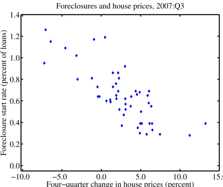
Our third method for estimating the losses draws on the past foreclosure experience of individual regions that have seen significant nominal home price declines. While
Exhibit 3.5 A Look at Three Regional Housing Busts
80 85 90 95 100 105 110
91 92 93 94 95 96 97 98 99 00
0.0 0.1 0.2 0.3 0.4 0.5 0.6 0.7 0.8
Home Prices (left)
Foreclosure Rate* (right)
Index Percent
* 4-quarter moving average
Source: Mortgage Bankers Association, OFHEO
California:
80 85 90 95 100 105
1984 1986 1988 1990 1992 1994 1996
0.1 0.2 0.3 0.4 0.5 0.6 0.7
Home Price (left)
Foreclosure Rate* (right)
Index Percent
*4-quarter moving average
Source: Mortgage Bankers Association, OFHEO
80 85 90 95 100 105
1990 1991 1992 1993 1994 1995 1996 1997 1998
0.1 0.2 0.3 0.4 0.5 0.6 0.7
Home Prices (left) Foreclosure Rate* (right)
Index Percent
* 4-quarter moving average
Source: Mortgage Bankers Association, OFHEO
Massachusetts:
Exhibit 3.6 summarizes the experience of the three regional housing busts by indexing the foreclosure rate at the beginning of the episode to 100 and then tracing its evolution over the following decade. The average rate triples within several years, and this same tripling holds for each of the individual states. After peaking between years 2 and 6, foreclosures gradually fall back towards the original level. Moreover, the chart shows that the initial experience with the national foreclosure rate in the first year of the current downturn is roughly consistent with what we saw in the typical regional housing bust episode.
Exhibit 3.6 Foreclosures Triple in the Housing Bust
Hence, we conclude from our analysis that a housing downturn that resembled the three regional busts, with a 10–15% peak-to-trough home price fall, could triple the national foreclosure rate over the next few years. This would imply a rise from 0.4% in mid-2006 to 1.2% in 2008 or 2009. Once home prices recover, the foreclosure rate might gradually fall back toward 0.4%.
So what does this mean for the total amount of mortgage credit losses over the next few years? To calculate the incremental defaults, we cumulate the differences between the projected foreclosure rate and the 0.4% rate prevailing at the start of the downturn in mid-2006 over the entire mid-2006-2013 period. This is a simple way of adjusting for the fact that this framework does not allow us to isolate defaults on the stock of mortgages
outstanding in February 2008 from defaults on mortgages that have yet to be originated. We believe this is a conservative choice, as quality standards on mortgages originated over the next few years are likely to return to the pre-2004 levels. Hence, the vast majority of the defaults in coming years are likely to involve mortgages originated up to 2007.
These assumptions imply cumulative “excess” foreclosures of 13.5% of the currently outstanding stock of mortgages over the next few years.12 On a base of $11 trillion of 1-4 family mortgage debt, this implies cumulative foreclosure starts of $1.5 trillion. Not every mortgage entering the foreclosure process will end up as an outright repossession, as some homeowners will manage to become current on their payment, sell, or refinance
12
The calculation is that the foreclosure rate exceeds its baseline level by an average of 0.48 percentage points per quarter for a 7-year period, which implies cumulative excess foreclosures of 13.5%.
0 50 100 150 200 250 300 350 400 450
0 4 8 12 16 20 24 28 32 36 40
0 50 100 150 200 250 300 350 400 450
US Current Episode California Massachusetts Texas
Index Index
Source: Mortgage Bankers Association.
Quarters from Peak
before the home is repossessed. However, the percentage of all foreclosure starts that turn into repossessions — measured by the number of Real Estate Owned (REO) notices divided by the lagged number of Notices of Default (NoD) — rose to 68% in the first quarter of 2008 according to Data Quick, Inc., a real estate information company. Assuming that repossessions continue to average about two-thirds of all initiated foreclosures and the average loss severity is 50%, as is typical in a depressed housing market, we calculate that $1.5 trillion of foreclosure starts could translate into mortgage credit losses of about $500 billion.13 Moreover, if home prices fall by more than the 10–15% drop seen in the California, Massachusetts, and Texas busts, the losses could be significantly larger.
We conclude from our review that total mortgage credit losses on the currently
outstanding stock of mortgages could total around $500 billion. This is somewhat more than implied by most vintage-by-vintage analyses, unless these are adjusted aggressively for structural changes resulting from the decline in home prices, approximately in line with the losses implied by the ABX indexes(once we adjust the latter for losses on non-subprime mortgages), and somewhat less than the losses suggested by our state-by-state analysis (once we adjust this analysis for the likely larger home price decline). We reiterate that the uncertainty around our estimate is undoubtedly very high.
3.4 Allocating the losses
To allocate the losses to different types of institutions, we rely on two sources of information: 1) top-down data on the mortgage exposures of different sectors and 2) bottom-up data on announced and estimated subprime exposures by company. In these calculations we exclude any losses on synthetic securities (such as credit default swaps), and this is important to recognize in comparing our estimates with others.
We first use data from the Federal Reserve Board and the Federal Deposit Insurance Corporation to allocate the total outstanding mortgage debt to different sectors. For each part of the “leveraged sector” — banks, savings institutions, credit unions, investment banks, government-sponsored enterprises, and finance companies — we add direct holdings of mortgages backed by 1-4 family homes and holdings of residential mortgage-backed securities (RMBS). Direct mortgage holdings by different sectors are available from the Federal Reserve’s Flow of Funds accounts. Holdings of RMBS by commercial banks and savings institutions are available from the FDIC. However, we need to estimate holdings of RMBS by credit unions, investment banks, and government-sponsored enterprises — which are not broken out separately in the Flow of Funds or FDIC data — by extrapolating from the asset-backed securities on their balance sheets and the share of RMBS in the total amount of outstanding asset-backed securities. As shown in Exhibit 3.7 below, our top-down calculation suggests that U.S. leveraged institutions hold 55% of all outstanding mortgage debt, either directly or via RMBS.
13
Our second approach relies on data from Goldman Sachs [2007] that are based on mortgage issuance, default, and prepayment data to calculate exposures to subprime mortgages across a broad range of leveraged and unleveraged institutions. We have made several adjustments to these data in order to estimate the share of all exposures held by U.S. as opposed to foreign leveraged institutions. First, we have reclassified $95 billion of subprime mortgage exposure held in the form of direct subprime loans by Household Finance, the U.S. subsidiary of HSBC, as a U.S. rather than a foreign exposure. This is because our definition of U.S. institutions in the macro data includes the U.S. subsidiaries of foreign banks. To the extent that the data for other foreign banks may also include exposures held by their U.S. subsidiaries, our estimates may understate the share of subprime exposures held by U.S. leveraged institutions.
Exhibit 3.7 Home Mortgage Exposures of U.S. Leveraged Institutions
Home Mortgage Debt Billion ($)
Total 11,136
US Leveraged Institutions 6,134
Commercial banks 2,984
Direct 2,012
RMBS 971
Savings Institutions 1,105
Direct 840
RMBS 265
Credit Unions 351
Direct 311
RMBS (estimate) 40
Brokers and Dealers 257
Direct 0
RMBS (estimate) 257
Government-Sponsored Enterprises 963
Direct 445
RMBS (estimate) 519
Finance Companies 474
Direct 474
RMBS 0
Source: Federal Reserve Board, FDIC. Authors' calculations
Second, we need to decide what percentage of hedge fund exposures estimated by the GS analysts refers to U.S. as opposed to foreign hedge funds. Unfortunately, no good
information is available on this issue. However, we believe it is safe to assume that U.S. hedge funds account for most subprime mortgage exposures by hedge funds globally and so we assume their share is 80%.
$250 billion, of our $500 billion estimate of credit losses on the currently outstanding stock of mortgages will hit U.S. leveraged institutions.14
Exhibit 3.8 Subprime Mortgage Exposures, Bottom-Up
4. Leverage and Amplification
We now attempt to reconcile the evidence presented in the last two sections. In doing so, we focus on three questions. First, can we understand how a shock of roughly $250 billion to the leveraged intermediary sector might cause the type of turmoil that we have documented? Second, can we simultaneously explain why other markets were not initially disturbed? Finally, what will the credit losses imply for lending by the intermediaries?
4.1 The mechanics of active balance sheet management
The first ingredient in our explanation relates to the risk management practices of modern financial intermediaries. Financial intermediaries manage their balance sheets actively in response to changes in anticipated risk and asset prices. When balance sheets are marked to market, asset price changes show up as changes in net worth and elicit reactions from financial intermediaries to changes in their net worth. Even in the absence of asset price changes, shifts in perceived risks will also elicit reactions from leveraged institutions. Moreover, financial intermediaries react in a very different way to the fluctuations in net
14
In Exhibit 3.8, we have not included the finance companies as part of the leveraged sector. Finance companies are not banks in the traditional sense, but arguably, they could be subject to the same forces in the adjustment of balance sheets. If we were to include finance companies in the leveraged sector the estimated impact of deleveraging to be reported below will be even higher.
Total reported sub-prime exposure
Percent of reported exposure
U.S. Investment Banks 75 5%
U.S. Commercial Banks 250 18%
U.S. GSEs 112 8%
U.S. Hedge Funds 233 17%
Foreign Banks 167 12%
Foreign Hedge Funds 58 4%
Insurance Companies 319 23%
Finance Companies 95 7%
Mutual and Pension Funds 57 4%
US Leveraged Sector 671 49%
Other 697 51%
Total 1,368 100%
Note: The total for U.S. commercial banks includes $95 billion of mortgage exposures by Household Finance, the U.S. subprime subsidiary of HSBC. Moreover, the calculation assumes that U.S. hedge funds account for four-fifths of all hedge fund exposures to subprime mortgages.
worth as compared to households or non-financial firms. Indeed, there is a wealth of evidence dealing with the role of home prices in the monetary transmission mechanism (see Mishkin [2007a]). However, households tend not to adjust their balance sheets drastically to changes in asset prices. In general, leverage falls when total assets rise. For households, the change in leverage and change in balance sheet size are negatively correlated.
However, the picture for financial intermediaries is very different. There is a positive relationship between changes in leverage and changes in balance sheet size. Far from being passive, financial intermediaries adjust their balance sheets actively and do so in such a way that leverage is high during booms and low during busts. Leverage is procyclical in this sense (Adrian and Shin [2007, 2008]). For financial intermediaries, their models of risk and economic capital dictate active management of their overall value at risk (VaR) through adjustments of their balance sheets. Value at risk is a numerical estimate of an institution’s “approximately” worst-case loss, in the sense that anything beyond this worst-case loss happens only with some benchmark probability.
Let V be the value at risk per dollar of assets held by a bank15. The total value at risk of the bank is given by V×A where A is total assets. Then, if the bank maintains capital E to meet total value at risk, we have E = V×A. Hence, leverage L satisfies
L = A/E = 1/V
Procyclical leverage can be traced directly to the counter-cyclical nature of value at risk. Leverage is high when values at measured risks are low — which occurs when financial conditions are buoyant and asset prices are high. Leverage is low in the troughs of the financial cycles, reflecting increased volatility of asset prices as well as increased correlation of asset returns.
Exhibit 4.1 plots the value-weighted quarterly change in leverage and change in assets for the five major U.S. investment banks up to 2008 Q116. Leverage is defined as the ratio of total assets to book equity. Two features stand out. First, leverage is procyclical.
Leverage increases when balance sheets expand, and leverage falls when balance sheets contract. Second, there is a striking contrast between the observation for 1998 Q4 associated with the LTCM crisis and the credit crisis that began in 2007. While balance sheets contracted sharply in 1998, there had not (at least through 2008 Q1) been a comparable contraction of balance sheets during this latest crisis. Indeed, it is one of our central contentions that understanding the reasons for the difference between 1998 and 2007 holds the key to unlocking some of the mysteries surrounding the severe pressures evident in the interbank credit market during the period from August 2007 to the spring of 2008.
15
Formally, the value at risk (VaR) associated with some time horizon T is the smallest non-negative number V such that the estimated probability that a bank’s loss is greater than V is less than some benchmark probability p. Value at risk is used widely by financial institutions and by regulators, and is incorporated into the Basel capital rules. We use “value at risk” to include the expected losses as well as the unexpected losses. Thus, V should be seen as including the expected losses.
16
Exhibit 4.1 Quarterly Changes in Assets and Leverage of U.S. Investment Banks
The leverage ratios of commercial banks is typically much lower — at around 10-12 — than that of investment banks (which have leverage ratios of roughly 20–25). However, the relationship between total assets and leverage reveals a similar picture to that given by the investment banks. Exhibit 4.2 plots the relationship between the quarterly change in total assets and the quarterly change in leverage for the five largest U.S. commercial banks — Bank of America, JP Morgan Chase, Citibank, Wachovia, and Wells Fargo — over the period 1988 Q1 to 2008 Q1. One important issue that arises in studying the banks is that each of them has been involved in multiple mergers and acquisitions over this period, so we have adjusted the data to remove these effects.17
Commercial banks also exhibit the positive relationship between changes in assets and changes in leverage. Investment bank balance sheets consist largely of very short-term claims (such as repurchase agreements and reverse repurchase agreements), so that their balance sheet values approximate the marked-to-market values of the underlying
securities. The same is not true for the commercial bank balance sheets, since loans are carried at face value. Thus, the scatter chart for commercial banks should be interpreted with some caution. Nonetheless, it is interesting to see that through 2008 Q1 the
commercial banks had also not shown signs of deleveraging, and in fact leverage actually rose in the first quarter of 2008. This stands in contrast to the experience in the past two recessions, where there was at least one quarter during which shrinking balance sheets were accompanied by falling leverage.
17
For instance, if banks A and B merge in quarter t so that bank B disappears, we compute the growth rate in assets and leverage by forming a combined bank in quarter t-1.
2007Q3
1998Q4
-0.20 -0.15 -0.10 -0.05 0.00 0.05 0.10 0.15 0.20
-0.2 -0.15 -0.1 -0.05 0 0.05 0.1 0.15 0.2
Leverage Growth (Quarterly)
Source: SEC
Note: Growth rates are assets-weighted.
2007Q4 2008Q1
Total As
set Growth
Exhibit 4.2 Changes in Leverage and Assets for Major U.S. Commercial Banks
-0.03 -0.02 -0.01 0 0.01 0.02 0.03 0.04 0.05 0.06
-0.08 -0.06 -0.04 -0.02 0 0.02 0.04 0.06
Leverage Growth (Quarterly)
T
o
ta
l A
s
s
e
t
G
ro
w
th
(
Q
u
a
rte
rl
y
)
Asset Growth and Leverage Growth For Top 5 U.S. Commercial Banks (1988-2008)
Note: Data are adjusted for mergers.
= 9/30/2007 = 12/31/2007 = 12/31/2001
= 12/31/1990. = 3/31/08
The adjustment of leverage has aggregate consequences that may lead to the amplification of the financial cycle. Consider a simple example. Take a financial
intermediary that manages its balance sheet actively so as to maintain a constant leverage ratio of 10. The hypothesis that the intermediary has a constant leverage target is for clarity of the illustration only. Our numerical estimates on credit contractions that follow later in the report recognize the possible role of deleveraging.
Thus, for this illustration only, suppose that the intermediary targets constant leverage of 10. Suppose the initial balance sheet is as follows. The intermediary holds 100 worth of assets (securities, for simplicity) and has funded this holding with debt worth 90.
Assets Liabilities
Securities, 100 Equity, 10
Debt, 90
Assume that the price of debt is approximately constant for small changes in total assets. First, let’s assume the price of securities increases by 1% to 101.
Assets Liabilities
Securities, 101 Equity, 11
Leverage then falls to 101/11 = 9.18. If the bank targets leverage of 10, then it must take on additional debt of D to purchase D worth of securities on the asset side so that
assets / equity = (101+ D)/11 = 10
The solution is D = 9. The bank takes on additional debt worth 9, and with the proceeds purchases securities worth 9. Thus, an increase in the price of the security of 1 leads to an increased holding worth 9. The demand curve is upward-sloping. After the purchase, leverage is now back up to 10.
Assets Liabilities
Securities, 110 Equity, 11
Debt, 99
The mechanism works in reverse, on the way down. Suppose there is shock to the
securities price so that the value of security holdings falls to 109. On the liabilities side, it is equity that bears the burden of adjustment, since the value of debt stays approximately constant.
Leverage is now too high (109/10 = 10.9). The bank can adjust down its leverage by selling securities worth 9, and paying down 9 worth of debt. In this way, a fall in the price of securities leads to sale of securities. The supply curve is downward-sloping. The new balance sheet is hence restored to where it stood before the price changes and leverage is back down to the target level of 10.
Assets Liabilities
Securities, 100 Equity, 10
Debt, 90
Leverage targeting entails upward-sloping demands and downward-sloping supplies. The perverse nature of the demand and supply curves is even stronger when the leverage of the financial intermediary is pro-cyclical — that is, when leverage is high during booms and low during busts. If, in addition, there is the possibility of feedback, then the
Assets Liabilities
Securities, 109 Equity, 10
adjustment of leverage and of price changes will reinforce each other in an amplification of the financial cycle.
Exhibit 4.3 The Leverage Circle
Target Leverage
Increase B/S Size Stronger Balance
Sheets
Asset Price Boom
Target Leverage
Weaker Balance
Sheets Reduce B/S Size
Asset Price Decline
If greater demand for the asset tends to put upward pressure on its price, then there is the potential for feedback in which stronger balance sheets trigger greater demand for the asset, which in turn raises the asset’s price and leads to stronger balance sheets. The mechanism works in reverse in downturns. If greater supply of the asset tends to put downward pressure on its price, then weaker balance sheets lead to greater sales of the asset, which depresses the asset's price and leads to even weaker balance sheets.
The balance sheet perspective gives new insights into the nature of financial contagion in the modern, market-based financial system. Aggregate liquidity can be understood as the rate of growth of aggregate balance sheets. When financial intermediaries’ balance sheets are generally strong, their leverage is too low. The financial intermediaries hold surplus capital, and they will attempt to find ways in which they can employ their surplus capital. In a loose analogy with manufacturing firms, we may see the financial system as having “surplus capacity.” For such surplus capacity to be utilized, the intermediaries must expand their balance sheets. On the liabilities side, they take on more short-term debt. On the asset side, they search for potential borrowers that they can lend to. Aggregate