STATIC AND DYNAMIC LOCATION OF VARIABLE IMPEDANCE DEVICES FOR STABILITY STUDIES

©2013 Science Publication

doi:10.3844/ajassp.2013.497.506 Published Online 10 (5) 2013 (http://www.thescipub.com/ajas.toc)

Corresponding Author: Magaji, N., Department of Electrical Engineering, Faculty of Engineering, Bayero University, Kano, Nigeria

STATIC AND DYNAMIC LOCATION OF VARIABLE

IMPEDANCE DEVICES FOR STABILITY STUDIES

1

Magaji, N.,

M.W. Mustafa,

Ado Dan-Isa and

A.U. Lawan

1

Department of Electrical Engineering, Faculty of Engineering, Bayero University, Kano, Nigeria 2_{Department of Power System, Faculty of Electrical Engineering, Universiti Teknologi Malaysia, Malaysia}

Received 2012-03-15, Revised 2012-09-26; Accepted 2013-05-31

ABSTRACT

This study used the concept of model controllability and observability in product form called residue factor to find the best location of Thyristor-Controlled based series and shunt devices called variable impedance devices. The success of this controller depends on its best possible location in busbar or line of power system network. The method is based on the relationship between the parameters of variable impedance devices to the vital modes. Linearization of non linear model of Power system and the thyristors based FACTS devices provide mens of computing residue factor and singular value factor. The location of variable impedance or thyristors based controllers have been calculated for the base case only. The usefulness of the these methods of placement considered 16 machines, 68 bus systems.

Keywords: Thyristor-Controlled Series Compensator (TCSC), Static Var Compensator (SVC), New England Test System (NETS), New York Power System (NYPS)

1. INTRODUCTION

FACTS devices based on Variable impedance devices or thyristors based controllers includes Static VAR Compensators (SVCs) and Thyristor-Controlled Series Capacitors (TCSC) can improve power control and system damping (Nazarpour et al., 2006; Magaji and Mustafa, 2010). Positioning of these devices n large power system is very importanc in terms of controlling of system modes, therefore, there is need to consider several conditions in dealing with this difficulty. Among the factors to take into accounts are (Pal and Chaudhuri, 2005; Magaji and Mustafa, 2009a; 2009b; Larsen et al., 1995; Hassan et al., 2010):

• Identification of busber for shunt FACTs devices

• Branches or lines for series FACTs devices

• Best stabilizing signals for supplementary controllers

Application of FACTS devices for evaluating system damping using various techniques are reported in

the literature (Pal and Chaudhuri, 2005; Magaji and Mustafa, 2009a; 2009b; Larsen et al., 1995; Hassan et al., 2010; Mustafa and Magaji, 2009; Sadikovic et al., 2006; Milano, 2007) and the usefulness of damping the oscillations depends on the location of FACTS controllers.

Sadikovic et al. (2006) adopted the approch of location index for efficient damping, to find suitable location for damping inter-area mode of oscillations. The authors consider only one FACTs controller based on single operating condition.

particular interest when the issue of system dmping is tking into ccount.

In this study, the approach adopted details the loction of SVC and TCSC devices based on model residue factor and it has been compared with static approach based on Singular Value Decomposition (SVD) adopted from (Ekwue et al., 1999). The proposed methods have been tested on a reduced order equivalent of the interconnected New England Test System and New York Power System. The effectiveness of the proposed method has been demonstrated through the time domain simulation in matlab software.

2. MATERIALS AND METHODS

2.1. Formulation of the State Equation

Multi-machine power system dynamic behavior in a smll signals model is usually expressed as a set of non-linear Differential and Algebraic (DAE) equations. The high frequency network and stator transients are usually ignored when the analysis is focused on low frequency electromechanical oscillations. The initial algebraic variables such as bus voltages bus angles and some control variables are obtained through a standard power flow solution (Milano, 2007). The state model given by (Hassan et al., 2010) is considered to represent system dynamic behaviour. In this model, the power system is seen as constituted of dynamic subsystems interacting through the transmission network. Two types of dynamic subsystems have so far been taken into account, that is to say synchronous machines and thyristor-controlled devices. The dynamic behaviour of system is expressed in (DAE) as shown in Equation 1-3 after it has been linearized around the equilibrium point:

(

)

f x, z, u ɺ

x= (1)

(

)

0=g x, z, u (2)

(

)

y=h x, z, u (3)

Linearizing (1) to (3) around the equilibrium point {x0, z0 u0) gives the following Equation 4-6:

f f f

x x z u

x z u

∂ ∂ ∂

∆ = ∆ + ∆ + ∆

∂ ∂ ∂

ɺ (4)

g g g

0 x z u

x z u

∂ ∂ ∂

= ∆ + ∆ + ∆

∂ ∂ ∂ (5)

h h h

y x z u

x z u

∂ ∂ ∂

= ∆ + ∆ + ∆

∂ ∂ ∂ (6)

Elimination of algebraic variable vector ∆z from Equation 4-6, gives Equation 7-13:

1 1

1 1 x A x B u y C x D u

∆ = ∆ + ∆

∆ = ∆ + ∆ (7)

where, A1 is a system matrix, B1 and C1 are the input and output-vector matrixs, respectively. Let λI = σI +jωi be the i-th eigenvalue of the state matrix A1. The real part of the eigenvalues gives the damping and the imaginary part gives the frequency of oscillation. The relative damping ratio is given by:

2 2 = −σ

ζ

σ + ω (8)

If the state space matrix A1 has n distinct eigenvalues and Λ, Φ and ψ below are the diagonal matrix of eigenvalues and matrices of right and left eigenvectors, respectively: 1 1 1 A A −

Φ = ΦΛ

Ψ = ΛΨ⇒_{Ψ = Φ} (9)

In order to modify a mode of oscillation by feedback, the chosen input must excite the mode and it must also be visible in the chosen output. The measures of those two properties are the controllability and observability, respectively. The modal controllability and modal observability matrices are defined as follows:

1 m 1 m 1 B B C C − = Φ

= Φ (10)

The mode is uncontrollable if the corresponding row of the matrix Bm is zero. The mode is unobservable if the corresponding column of the matrix Cm is zero. If a mode is either uncontrollable or unobservable, feedback between the output and the input will have no effect on the mode. The open loop transfer function of a SISO (single input single output) system is:

1 1 1 1 y(s)

G(s) C (sI A ) B u(s)

− ∆

= = −

∆ (11)

N

1 i i 1

i 1 i N

i

i 1 i

C B G(s) (s ) R (s ) = = φ ψ = − λ = − λ

∑

∑

Each term in the nemerator, Ri, of the summation is a scalar called residue. The residue Ri of a specific mode i gives the measure of that mode’s sensitivity to a feedback between the output y and the input u; it is the product of the mode’s observability and controllability. When applying the feedback control, eigenvalues of the initial system G(s) are changed. It can be proven, that when the feedback control is applied, the shift of an eigenvalues can be calculated by:

i = R H( )i i

∆λ λ (13)

It can be observed from (19) that the shift of the eigenvalue caused by the controller is proportional to the magnitude of the corresponding residue.

2.2.Variable Impedance Models

2.2.1. TCSC Model

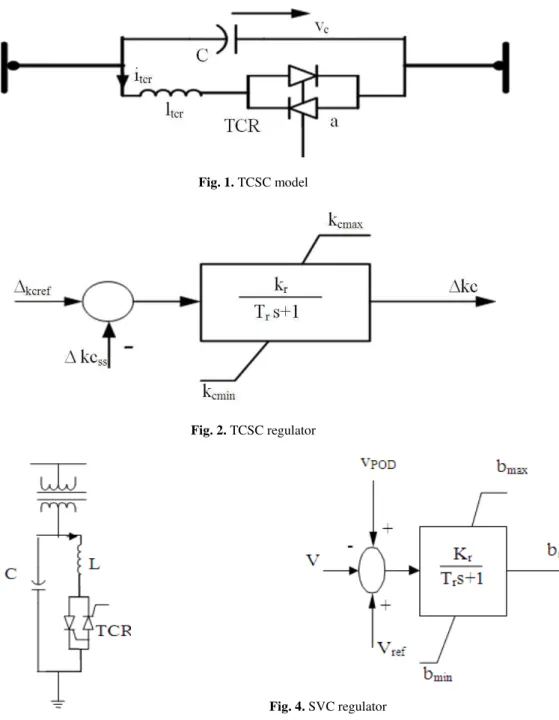
A tyristor Controlled Seres Cpacitor module consists of a fixed series Capacitor (FC) in shunt with a Thyristor Controlled Reactor (TCR) as shown in Fig. 1. The Thyristor Controlled Reactor is created by a reactor in series with a bi-directional thyristor valve that is fired with an angle ranging between ninety degree and one eighty degree with respect to the capacitor voltage (Magaji et al., 2010).

2.3. Dynamic Model

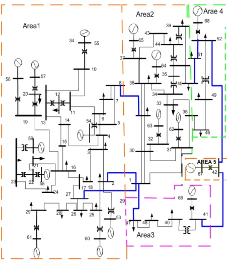
The dynamic characteristics of the TCSC is assumed to be model by a first order time constant in place of the response time of the TCSC control circuit which is expressed a Equation 14:

(

)

c cref c css tcsc

1

k = k k k

T

∆ɺ ∆ − ∆ + ∆ ₍₁₄₎

The low frequency dynamic model (Magaji and Mustafa, 2009a) of a thyristor controlle series capacitor is given in Fig. 2. The symbol kc is the smalll change in value of kC about the nominal value of 50% compensation. kcref is the reference setting which is augmented by kcss within a limit of kcmax = 0.1 and

kmin = -0.1 in the company of supplementary damping controller (Chaudhuri and Pal, 2004).

2.4. SVC Devices

The Static VAr Compensator (SVC) is a prallel device whose main work is to control the voltage at a chosen bus by appropriately regulating its equivalent reactance. A basic circuit consists of a cascade capacitor bank, C, in shunt with a thyristor-controlled reactor, L, as shown in Fig. 3. In practice the SVC can be seen as an regulating reactance (Nazarpour et al., 2006) that can perform both inductive and capacitive compensation.

2.5. Dynamic Model

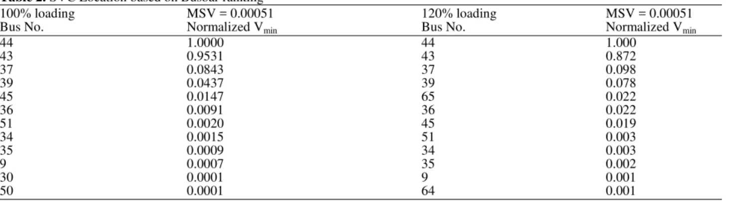
The low frequency dynamic model is shown in Fig. 4; the model that is used here assumes a time constant regulator. In this model, a total reactance bSVC is assumed and the following differential equation holds (Milano, 2007; Magaji and Mustafa, 2008) Equation 15:

SVC r ref POD SVC r

bɺ = (K (V + v - V ) - b )/T (15)

The regulator has an anti-windup limiter, thus the reactance bSVC is locked if one of its limits is reached and the first derivative is set to zero (Milano, 2007; Magaji and Mustafa, 2008).

The auxiliary input POD is used to connect the POD controller for damping oscillations while Vref to maintain acceptable voltage at the SVC bus. TCR of 150MVAr is normally connected in parallel with fixed capacitor of 200MVAr correspond to a limit of 2.0pu to -1.0 pu voltage (Milano, 2007).

2.6. Computational Procedure for Residue Factor

The allocation algorithm can be formulated as follows:

• Perform free fault power flow and eigenvalues analysis

• Identify inter area mode

• Model the FACTS device

• Place the TCSC in series and SVC in shunt in the model

• Perform power flow and obtain linear model of the system

• Calculate residue factor based on SVC/TCSC location under all operating conditions

Fig. 1. TCSC model

Fig. 2. TCSC regulator

Fig. 3. SVC model

2.7. Singular Value Decomposition

SVD consists of finding the eigenvalues and eigenvectors of system ether express in state space or transfer function of SISO |G(s)| system which is more significant than eigenvalues techniques in terms of magnitude of According to (Ekwue et al., 1998) the SVD theorem is stated as follows.

Fig. 4. SVC regulator

Let m n

r

G∈C × There exist unitary matrices U1∈Cm×m V1∈Cn×n such that G = U1ΣV1H.

Where:

1 r 1 2 r

s 0 =

0 0

s diag( ,..., ) with ... 0.

 

∑  

 

Fig. 5. One-line diagram for 16 machine 68-bus system

U1 is a matrix of output singular vectors ui and V1 is a unitary matrix of input singular vectors vi.

V1H is the complex conjugate transpose of V1. The singular values are positive square roots of the eigenvalues of GHG which are real because the matrix GHG is symmetric, or in other words Equation 16:

H

i i

(G)=σ λ(G G) (16)

The input and output directions are connected through the singular value σi.σ1 is the first singular value hence called maximum singular value, similarly σr is the minimum singular value.

2.8. Minimum Singular Value Decomposition

The minimum singular value, σmin could be used as an indicator of voltage stability. The closer to voltage instability the current operating condition is, the smaller

the singular value (Chaudhuri and Pal, 2004). Considering the power flow Equation 17:

P =J

Q V

∆ ∆θ

   

_∆  _∆ 

    (17)

Where:

P = Implies active power Q = Implies reactive power

Θ = Node angles

V = Node voltage magnitudes and

J = Means the Jacobian matrix of power flow equations

According to the singular value decomposition theorem, the Jacobian matrix, J, is defined as Equation 19:

i

n

T T

i i i 1

J=V W V W

=

where, Λi in Equation 18 are the singular values, Vi and Wi are the left and right singular vectors respectively of a power system model, while n is the number of system buses or lines.

As J is a non-singular matrix and V, W are unitary matrices, the effect of small changes in the active and reactive power injections on the bus voltage angles and magnitudes can be written as:

n

1 -1 T

i i i=1

P P

J = W V

V Q Q

−

∆θ ∆ ∆

     

= σ

_∆  _∆  _∆ 

   

∑

When power system is close onto voltage collapse, the system characteristic is dominated by the minimum singular value σ min and its corresponding left and right singular vectors, that is described in Equation 20 and 21:

-1 _T

min min min P W V V Q ∆θ ∆     = σ _∆  _∆ 

    (20)

Assuming:

-1

min min min P

V W

Q V

∆ ∆θ

   

= ⇒ _{= σ}

_∆  _∆ 

    (21)

• From the power flow solution the smallest singular value will be a point to indicte a closeness to static stability limit

• The highest value in Wmin indicate the most responsive bus voltages and this indicate the weak buses

• The highest value in T min

V correspond to the most sensitive direction for changes of active and reactive power injections

2.9. Static Placement Based on Singular Value

Decomposition

2.9.1. SVC Locations based on SVD

In this study, the principle used for findng best location of SVC controllers is based on ranking of voltage-weak buses. The value right singular vector with respect to the minimum singular value is considered as an indicator for ranking buses

The highest valuein Vmin indicate the most responsive bus voltage (critical bus) hence, under any operating condition; those bus that is highest on the

ranked list is bus where SVC should be located for reactive power compensation to help voltage stability (Ekwue et al., 1999).

2.10. TCSC Locations Based on SVD

The loction of TCSC is based on reactive power losses of transmission line for voltage stability. The transmission line reactive power losses are the measurable information of transmission lines about voltage stability. The line with the highest change of reactive power loss is the most susceptible to voltage stability. From Equation 22, the incremental changes in reactive power loss for both the sending and receiving ends of transmission lines Qloss (i), can be calculated as defined in the study of Ekwue et al. (1999). The line is ranks based on participation factor for a transmission line which is defined as:

[

]

i

j Qloss(i)

Lf = j branches Qloss(j)

∆ _∈

∆

∑

3.

RESULTS

Modal analysis shows that, in the base case, there is a critical interarea mode with low damping ratio of 0.028438, having eigenvalues -0.15066±j5.2957. Analysis of phase angle of the right eigen vectors shows that in this inter-area mode, generator G15, which is in a neighborhood of NYPS, is oscillating against a cluster of generators G13 in NYPS, G9 and G6 in NETS. For this critical mode, the proposed residue, corresponding to the weakly damped inter-area mode, computed for SVC and TCSC are given in Table 1. These indices are expressed in the normalized form, only few buses/lines, having significant value of the residue of the two types of FACTS controllers for the base case were determined. Table 1 shows that lines between buses 51-52 and bus 28 are the optimal locations for TCSC and SVC device respectively.

Hankel Singular Value (HSV) analysis was carried out to find the suitable feedback signals for the FACTS controllers (Magaji and Mustafa, 2009b). Line 51-50 real power flow which is a local signal has been taken as the feedback signal for the TCSC supplementary controller. Current magnitude of Line 27-28 from bus 27 is taken as the feedback signal for the SVC supplementary controller.

different operating conditions, that is base case at 100% loading and contingency case at 120% loading the SVD method indicates that the load bus 44 is the Weakest bus hence best location of SVC device. Similarly optimal location of TCSC based on SVD by ranking of critical transmission lines in terms of voltage stability is found to be line between bus 25 and 26 as shown in Table 3.

3.1. Performance Evaluation

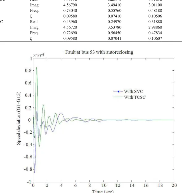
To test the effective location, a step input was applied to the exciter of generator G1 to observe the impact of FACTS controllers on the inter-area mode damping. It can be seen from Fig. 6 the inter-area mode, with SVC device, has settled in 9-10 s. The damping is reduced to a minimum and settled in about 5s though with small oscillations after TCSC placed in line 51-52 compared to SVC placement.

Table 4 shows the eigen-value analysis of the system without any device, with TCSC and with SVC device. From this table the damping of different modes for both the variable impedance devices has been demonstrated.

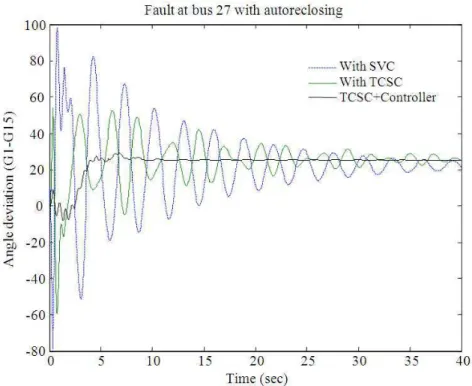
For testing transient stability with variable impedance controllers placed in the system, a three-phase fault was applied at bus 27 for 120 ms, speed deviation and the rotor angle difference between generators G1 and G15, ware plotted and are shown in Fig. 6 and 7.

Table 1. Residue factor of FACTS device for 68-bus test system TCSC Placement SVC Placement --- --- Line connection N RF Bus No. N RF

2 3 0.17 4 0.089

2 25 0.27 5 0.090

10 11 0.10 6 0.089

10 13 0.12 8 0.096

16 19 0.21 11 0.082

21 22 0.23 14 0.084

23 59 0.47 16 0.078

9 36 0.25 18 0.083

36 37 0.63 28 1.000

34 36 0.75 39 0.178

44 45 0.11 40 0.398

45 50 0.45 43 0.158

51 52 1.00 45 0.290

50 51 0.19 49 0.244

41 40 0.15 51 0.131

Table 2. SVC Location based on Busbar ranking

100% loading MSV = 0.00051 120% loading MSV = 0.00051

Bus No. Normalized Vmin Bus No. Normalized Vmin

44 1.0000 44 1.000

43 0.9531 43 0.872

37 0.0843 37 0.098

39 0.0437 39 0.078

45 0.0147 65 0.022

36 0.0091 36 0.022

51 0.0020 45 0.019

34 0.0015 51 0.003

35 0.0009 34 0.003

9 0.0007 35 0.002

30 0.0001 9 0.001

50 0.0001 64 0.001

Table 3. TCSC location based on transmission line rankings for the base case

Normalized Transmission line ranking Bus No. Bus No. participating factor

1 25 26 1.00

2 14 15 0.86

3 41 40 0.63

4 17 27 0.52

5 50 51 0.49

6 21 22 0.45

7 30 32 0.43

8 42 41 0.41

9 3 18 0.39

10 19 20 0.38

11 48 40 0.36

12 1 47 0.35

13 3 4 0.31

14 26 28 0.28

Table 4. Damping ratio under different Conditions

Inter-area modes Mode1 Mode2 Mode3 Mode4

Without FACTS Real -0.43960 -0.24800 -0.31910 -0.21020

Imag 4.56790 3.53920 2.99230 2.18010

Freq. 0.73040 0.56470 0.47895 0.34858

ζ 0.09580 0.06990 0.10605 0.09598

With TCSC Real -0.43970 -0.25970 -0.31810 -0.21130

Imag 4.56790 3.49410 3.01100 2.18002

Freq. 0.73040 0.55760 0.48188 0.35178

ζ 0.09580 0.07410 0.10506 0.09648

With SVC Real -0.43960 -0.24970 -0.31880 -0.21030

Imag 4.56720 3.53780 2.98860 2.17440

Freq. 0.72690 0.56450 0.47834 0.34767

ζ 0.09580 0.07041 0.10607 0.09624

Fig. 6. Speed deviation of (G1-G15)

It can be observed from these figures that the response of the TCSC device with supplementary controller produce very low oscillation compared with TCSC and SVC device only. The response is poor for the

Fig. 7. Angle difference between generators G1 and G 15

4.

DISCUSSION

The proposed methodologies are tested on a dynamic model of the reduced order equivalent of the interconnected New England Test System (NETS) and New York Power System (NYPS). The test system consists of 68 buses, 16 machines and five areas as shown in Fig. 5. The data are adopted from (Pal and Chaudhuri, 2005).

5. CONCLUSION

A set of Residue indices have been proposed in this study in order to find the optimal location of TCSC and SVC for enhancing damping of small signal oscillations and, thus, improving the system stability. Residue indices for the placement of FACTS controllers have been found corresponding to a critical inter-area mode in case of 68-bus systems. These indices have been computed for the base case only. Best location of FACTS was also found on the basis of static criteria utilizing singular Value decomposition for voltage stability. It was establish that these two factors provide different optimal locations of the FACTS controllers.

TCSC controller in the study is found to be more effective in improving the transient performance compared with the SVC device.

Application studies on a complex power system have shown that SVC and TCSC have the potential to substantially increase system damping. All the simulations were done with PSAT, PST or MatNet Eig toolbox in MATLAB.

6. ACKNOWLEDGEMENT

The reschers would like to express their appreciation to the Universiti Teknologi Malaysia (UTM) and Ministry of Science Technology and Innovation (MOSTI) for funding this research.

7. REFERENCES

Chaudhuri, B. and B.C. Pal, 2004. Robust damping of multiple swing modes employing global stabilizing signals with a TCSC. IEEE Trans. Power Syst., 19: 499-505. DOI:10.1109/TPWRS.2003.821463 Ekwue, A.O., A.M. Chebbo, M.E. Bradley and H.B.

Ekwue, A.O., H.B. Wan, D.T.Y. Cheng and Y.H. Song, 1999. Singular value decomposition method for voltage stability analysis on the National Grid System (NGC). Int. J. Elect. Power Energy Syst., 21: 425-432. DOI: 10.1016/S0142-0615(99)00006-X

Hassan, L.H., M. Moghavvemi and H.A.F. Mohamed, 2010. Power system oscillations damping using unified power flow controller-based stabilizer. Am. J. Applied Sci., 7: 1393-1395. DOI: 10.3844/ajassp.2010.1393.1395

Larsen, E.V., J.J. Sanchez-Gasca and J.H. Chow, 1995. Concepts for design of FACTS controllers to damp power swings. IEEE Trans. Power Syst., 10: 948-956. DOI:10.1109/59.387938

Lee, S. and C.C. Liu, 1994. An output feedback static var controller for the damping of generator oscillations. Elect. Power Syst. Res., 25: 9-16. DOI: 10.1016/0378-7796(94)90043-4

Magaji, N. and M.W. Mustafa, 2009a. Optimal location and signal selection of SVC device for damping oscillation. Int. Rev. Model. Simulat., 2: 144-151. Magaji, N. and M.W. Mustafa, 2009b. Optimal thyristor

control series capacitor neuro-controller for damping oscillations. J. Comput. Sci., 5: 983-990. DOI: 10.3844/jcssp.2009.980.987

Magaji, N. and M.W. Mustafa, 2010. Determination of best location of FACTS devices for damping oscillations. Int. Rev. Elect. Eng., 5: 1119-1126. Magaji, N. and M.W.B. Mustafa, 2008. Application of

SVC device for damping oscillations based on eigenvalue techniques. Int. J. Power Energy Artif. Intell., 1: 42-49.

Magaji, N., M.W. Mustafa and Z. Muda, 2010. Signals selection of SVC device for damping oscillation. Proceedings of IEEE 10th International Conference on Information Science, Signal Processing and their Applications (ISSPA), May 10-13, IEEE Xplore Press, Kuala Lumpur, pp: 786-789. DOI: 10.1109/ISSPA.2010.5605511

Milano, F., 2007. Documentation for PSAT Version 2.0.0 β.

Mustafa, M.W. and N. Magaji, 2009. Optimal location of static var compensator device for damping oscillations. Am. J. Eng. Applied Sci., 2: 353-359. DOI: 10.3844/ajeassp.2009.353.359

Nazarpour, D., S.H. Hosseini and G.B. Gharehpetian, 2006. Damping of generator oscillations using an adaptive UPFC-based controller. Am. J. Applied

Sci., 3: 1662-1668. DOI:

10.3844/ajassp.2006.1662.1668

Pal, B. and B. Chaudhuri, 2005. Robust Control in power Systems. 1st Edn., Springer, USA., ISBN-10: 038725949X, pp: 190.

Sadikovic, R., P. Korba and G. Andersson, 2006. Self-tuning controller for damping of power system oscillations with FACTS devices. Proceedings of the IEEE Power Engineering Society General Meeting, (PESGM’ 06), IEEE Xplore Press, Montreal, Que. DOI:10.1109/PES.2006.1709473