Comparison of High Speed Congestion Control Protocols

(1)

International Journal of Network Security & Its Applications (IJNSA), Vol.4, No.5, September 2012

DOI : 10.5121/ijnsa.2012.4502 15

Jawhar Ben Abed

1

, Lâarif Sinda

2

, Mohamed Ali Mani

3

and Rachid Mbarek

2

1

Polytech Sousse, 2ISITCOM Hammam Sousse and 3ISTLS Sousse, Tunisia ba.jawhar@gmail.com

sindalaarif@gmail.com Mohamed.Ali.Mani@gmail.com

Rachid.Mba@hotmail.fr

A

BSTRACT

Congestion control limits the quantity of information input at a rate less important than that of the transmission one to ensure good performance as well as protect against overload and blocking of the network. Researchers have done a great deal of work on improving congestion control protocols, especially on high speed networks.

In this paper, we will be studying the congestion control alongside low and high speed congestion control protocols. We will be also simulating, evaluating, and comparing eight of high speed congestion control protocols : Bic TCP, Cubic TCP, Hamilton TCP, HighSpeed TCP, Illinois TCP, Scalable TCP, Compound TCP and YeAH TCP, with multiple flows.

K

EYWORDS

High-Speed, TCP protocols, Congestion Control, Performance, Multiple flows.

1. I

NTRODUCTION

In Internet, there are some machines responsible for transmitting data packets, and other that take off these packets from the queue. If the sender machine sends a data packet rate much more important than the rate of the receiver, network congestion is produced, hence, a congestion control will limit the quantity of input information with a lower rate than the transmission one to guarantee a good performance as well as a network protection against overloading and blocking. The high number of high speed congestion control protocols led us to prepare this research work, which focuses on evaluating and comparing high speed congestion control protocols. This paper is organized as follows:

In the second section we study the state of the art. In the third one, we present the architectures used as well as the curves and the performances evaluation for different high speed congestion control protocols.

2. S

TATE OF THE ART

Researchers have worked on the enhancement of high speed congestion control protocols. Practically every year, one or two protocols are implemented having for each one of them its own specific strengths and weaknesses.

Recently, the research works are interested in evaluating the performance of these protocols by comparing among 2 to 5 protocols with 1 to 12 flows [1] [2] [3] [4] [5] [6].

(2)

16

algorithm of HS-TCP is an AIMD Additive Increment cwnd = cwnd + a(cwnd) Multiplicative Decrement cwnd = (1- b(cwnd)) x cwnd, the values used for HSTCP are a(cwnd) in the interval of [1,72], b(cwnd) in the interval of [0.1,0.5] and low_window equals 38 packets. when cwnd is lower than low_window a(cwnd) = 1 and b(cwnd) = 0.5 thus the algorithm acts just like a standard TCP, in the case of a packet loss, the cwnd is reduced to 50%, when the cwnd reaches the high_window a(cwnd ) = 72 and b(cwnd)=1.

If there is an acknowledgment:

= 1 +_{2 × cwnd} cwnd <

= cwnd cwnd ≥

w = cwnd

Scalable TCP [8] : For this protocol the cwnd increases with 0.001, if a congestion is detected the cwnd reduces with 0.125 independently from the throughput and the packet size. This algorithm is a MIMD; Multiplicative Increase since the cwnd increases with 0.01 per acknowledgment, Therefore there is a total increase of 0.01 cwnd per RTT, and Multiplicative Decrease since the cwnd decreases with 0.125 per packet loss.

BIC TCP [9] : uses a function that allows to have a rapid increase of cwnd when its value is far from the maximal threshold Smax and to slowly decrease when having a value close to w_1. cwnd = (1 – ) × cwnd

With :

f ( ,cwnd) =

≤ 1 and cwnd < w or w ≤ cwnd < w + 1 < ≤ S !" and cwnd < w #$

%1 ≤ cwnd − w < S !"(1− ) S !" otherwise

cwnd : Current congestion window

S !" : Maximal threshold

S ,- : Minimal threshold

: Decrease factor usually equals 0.875

CUBIC TCP [10] : The name CUBIC refers to the function of the congestion window increase which is cubic, when receiving an ACK:

cwnd = C (T – K) ³ + Max_0#-1 When having a packet loss:

(3)

17 HTCP [11] : uses the duration since the last congestion rather than cwnd as information about the product delay bandwidth BDP. The increase parameter of AIMD (additive-increase/multiplicative-decrease) varies depending on . It also depends on the value of RTT which has provoked the unfairness among the competitor flows with different RTTs.

In case of receiving an ACK:

cwnd = cwnd + ( % ) 23(4) 0#-1

In case of packet loss:

cwnd = g (B) × cwnd

With :

f (Δ) = 8 1 Δ ≤ Δ9 max ;f<(Δ) T ,-,1> Δ > Δ9

g (B) = @ 0.5 D

E(FG ) – E(I) E(F) D > ΔE min JKLMN

KLOP ,0.8R otherwise

cwnd : Current congestion window : Increase parameter

: Decrease parameter

: Duration of time since the last congestion

9 : Threshold to change the mode low speed to highspeed T ,- : Minimal duration of sending and receiving packets T !" : Maximal duration of sending and receiving packets B(K + 1) : Maximal throughput reached before a congestion

f<(Δ) = 1 +10 ( - ₉) + 0,25 ( - ₉)²

Illinois TCP [12] : Similar to standard TCP, Illinois-TCP increases the congestion window by using two parameters and , it is based on packet loss to define the congestion window value, however the values of and are not constant by using the delays.

When receiving an ACK:

cwnd = cwnd + TUVW

Cwnd : Current congestion window C : Constant

T : Duration of time since the last congestion

(4)

18

When losing packets:

cwnd = (1- ) × cwnd

With :

= [(\_]) = ^ _]`a$ \] ≤ \ abG Wc deℎgh ijg

= [ (\_]) = @

_kV \] ≤ \

lm+ ln\] \ < \] < \m _]` deℎgh ijg

l =(Wo% W$) opq ocr

ocr% opq l =

(Wo% W$) opq ocr% opq - \

lm= opq_WWZ_Z_{% W}% ocr_b Wb ln= ocr_W_Z_{% W}% opq_b

_kV = _a a$

bG Wost , _]` = a$ abG W$ _kV = lm+ ln\ , _]` =lm+ ln\m

YeAH TCP [13] : the algorithm starts with the Slow Start if cwnd < ssthresh and Scalable TCP once cwnd reaches the ssthresh. This protocol uses two modes, fast mode and slow mode. In the case of the fast one, the congestion window increases aggressively, for the second mode, the protocol behaves similarly to Reno TCP. The mode is chosen according to the queue status. Having RTT_Evwx the minimal RTT measured by the sender and RTT_yz{ the minimal RTT estimated from the current window. The estimated delay is:

RTT|}~}~= RTT ,-− RTT•!€~

Thanks to this value, the number of packet on hold in the queue can be defined as follows:

Q = RTT|}~}~ × G = RTT|}~}~ × _RTTcwnd

And G is the throughput.

COMPOUND TCP[14]:Is a compilation of two approaches delay based and loss based with the congestion avoidance of TCP protocol. A new variable delay window (dwnd) was added wich gives the protocol more aggressive.

win = min (cwnd +dwnd, awnd) With :

dwnd(t+1)=ƒ

\ „\(e) + ;…. i„(e)a_{− 1>} _{i[\i[[ < †} (\ „\(e) − ‡. \i[[) i[ \i[[ ≥ † J i„(e). (1 − ˆ) −TUVWR ‰„ Š‹jg d[ Œ‹•Žge •djj

• i[ \i[[ < †: The link is free

(5)

g•ŒgŠeg\ =_•]–—UkV_˜™™ ; Expec

‹ŠeŽ‹• =_“””UkV; Actual; curre

’‹jg“””: estimation of trans

In case of receiving an ACK: cwnd = cwnd + _UkV

For the congestion avoidance :

In case of receiving an ACK: win(t+1) = win(t) + .wi In case of packet loss:

win(t+1) = win(t).(1- β)

3. S

IMULATION AND PERF

3.1. Architecture

In order to simulate the high spee shown in figure 1) composed of line of 1Gbps of bandwidth, the having a bandwidth of 200Mbps 100 packets [15]. The MSS siz capacities provoke congestion.

To evaluate the performances, w shown in figure 2) with a link cap

Figur

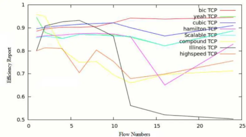
3.2. Efficiency

The efficiency (rate of utilization [16]. Mathematically, it is the div

ected; estimation of the throughput

rent throughput nsmission delay.

win(e)a

FORMANCES EVALUATION

peed congestion control protocols, we have chosen a t of a sender and a receiver linked together with two r he delay is 1ms. The routers are linked to each other

ps, the delay is equal to 98 ms and the queue capacit size equals 1460 bytes. The differences among the

Figure 1. Basic topology

, we have used 2, 4, 6, 8, 10, 12, 16 and 24 identica capacity of 1 Gbps and a delay of 1 ms.

ure 2. Topology with multiple flows

ion or performance) of a network is the percentage o division of the average throughput by the optimal throu

19

a topology (as o routers by a er with a line city is exactly e bandwidths

ical flows (as

(6)

20

An efficient network uses the maximum of capacity.

The following variable •_k is used as the average throughput of a flow i.

The throughput of a source with n flows is:

š =1_{„ › •}k V

kœ

We calculate the ratio between the average throughput and the optimal one which is the result of an ideal network performance:

• =_šš žŸ

We have used these two topologies to simulate the seven protocols for 1, 2, 4, 6, 8, 10, 12, 16 and 24 flows.

The efficiency calculus results are as mentioned in the following graph:

Figure 3. Efficiency for different flow numbers

3.3. Fairness

The fairness is the attempt of sharing the network capacities among users in a fair way.

For the purpose of measuring the fairness, one method is used in the networks field which is called the Maximin law proposed by Raj Jain [17]. Here is the procedure that allows us to calculate the fairness of a proposed algorithm:

Having an algorithm that provides the distribution v_, = [x , x ,…,x_-] instead of the optimal distribution v_¢£¤ = [x _,¢£¤, x _,¢£¤, … , x_-,¢£¤]. We calculate the standardized distribution for every source as follows:

(7)

21

Thus, the fairness index F equals the sum of distributions squared and divided by the square of sums:

We have used these two topologies to simulate the seven protocols for 1, 2, 4, 6, 8, 10, 12, 16 and 24 flows.

The fairness calculus results are as mentioned in the following graph:

Figure 4. Fairness for different flow numbers

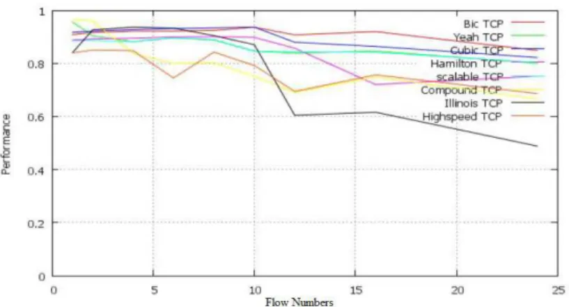
3.4. Performance

The performance of a congestion control algorithm is the relation between efficiency and fairness:

Performance = × E + (1 – ) × F With = [0,1.. 0,9], E the efficiency and F the fairness.

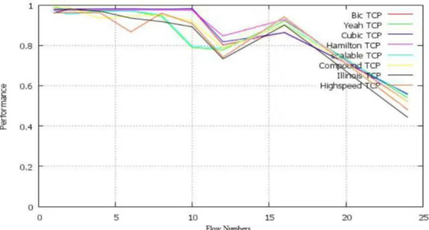
For the different algorithms, we have calculated the performances for a network rather efficient with = 0,8, a network rather fair with = 0,2 and a balanced network when = 0,5. The results for 1, 2, 4, 6, 8, 10, 12, 16 and 24 flows are as follows:

(8)

International Journal of Network

Figure 5.b. Perf

Figure 5.c. Perf

4. C

ONCLUSIONS

The high number of congestion field is always having changes a both of hardware and software algorithm that gives satisfying re During this research work, we sim 4, 6, 8, 10, 12, 16 and 24 flows. the fairness as well as the perform Basing on the simulation and the that:

• Some protocols perform wel • The network architecture ha • For 24 flows, all protocols a

k Security & Its Applications (IJNSA), Vol.4, No.5, Septem

erformance for different flow numbers ( = 0,5)

erformance for different flow numbers ( = 0,2)

on control algorithms never satisfied the researchers s and enhancements due to the users’ needs and the e

e in Telecommunications. Indeed, it is difficult to c results for all the architectures.

simulated eight high speed congestion control protoc s. We evaluated their performances by calculating the

rmance.

the high speed protocols performance evaluation, we ca

ell in some defined cases, but weak in others. has got an important impact on the protocols performa

are unfair.

tember 2012

22

rs. Since this e evolution of conceive an

ocols for 1, 2, the efficiency,

can conclude

(9)

23

• For 24 flows, the protocols: Bic TCP, Cubic TCP, Hamilton TCP, Scalable TCP and YeAH TCP are efficient.

Further work is required to evaluate the performances of these protocols by using Relentless TCP which will be the topic for a multitude of research works in the near future, particularly to define if the protocols that have more stability and take more time before falling another time in a new congestion such as Cubic TCP and Illinois TCP in order to check if they will well exploit the law that forms the basis of Relentless TCP which is the reduction of the congestion window with the number of lost segments. It will be also interesting to create a model that changes dynamically the congestion control protocols used in terms of flow number to better exploit the network capacities as well as studying the QoS.

R

EFERENCES

[1] R. Mbarek, M. T. BenOthman and S. Nasri. “Fairness of High-Speed TCP Protocols with Different Flow Capacities”. Journal Of Networks, Vol. 4, No. 3, pp. 163-169, May 2009. [2] S. Hemminger. “TCP testing – Preventing global Internet warming”. LinuxConf Europe, Sep.

2007.

[3] S. Ha, L. Le, I. Rhee and L. Xu. “Impact of Background Traffic on Performance of High-Speed TCP Variant Protocols”. The International Journal of Computer and Telecommunications Networking, Vol.51, May, 2007.

[4] M. Nabeshima and K. Yata. “Performance Evaluation and Comparison of Transport Protocols for Fast Long-Distance Networks”. IEICE Trans. Commun., Vol.E89-B, No.4, pp. 1273-1283, Apr. 2006.

[5] M. Weigle, P. Sharma and J. Freeman. “Performance of Competing High-Speed TCP Flows”. Networking 2006, LNCS 3976, pp. 476-487, 2006.

[6] M.A.Mani and R.Mbarek. “Performance Evaluation of High Speed Congestion Control Protocols”. IOSR Journal of Computer Engineering (IOSRJCE), Vol.3, Issue 1, PP 12-19, July-Aug. 2012.

[7] S. Floyd. “High-Speed TCP for Large Congestion Windows”. RFC 3649, Experimental, Dec. 2003.

[8] T. Kelly. “Scalable TCP : Improving Performance in High-Speed Wide Area Networks”. In Proceedings of PFLDnet, Geneva, Switzerland, Feb. 2003.

[9] L. Xu, K. Harfoush, and I. Rhee. “Binary Increase Congestion Control for Fast, Long Distance Networks”. In Proceedings of IEEE INFOCOM, Hong Kong, Mar. 2004.

[10] I. Rhee and L. Xu. “CUBIC: A New TCP-Friendly High-Speed TCP Variant”. In Proceedings of PFLDnet, Lyon, France, Feb. 2005.

[11] R. N. Shorten and D. J. Leith. “H-TCP : TCP for high-speed and long-distance networks”. In Proceedings of PFLDnet, Argonne, Feb. 2004.

[12] S. Liu, T. Basar and R. Srikant.,"TCP-Illinois : A Loss- and Delay-based Congestion Control Algorithm for High-Speed Networks", Performance Evaluation, 65(6-7) : 417-440, Mar. 2008. [13] A. Baiocchi, A. P. Castellani and F. Vacirca. “YeAH-TCP: Yet Another Highspeed TCP”.

PFLDnet, Roma, Italy, Feb. 2007.

[14] K.Tan, Q.Zhang and M.Sridharan “Compound TCP: A Scalable and TCP-Friendly Congestion Control for High-speed Networks”, May.2007.

(10)

24 [16] R. Mbarek, M. T. BenOthman and S. Nasri. “Performance Evaluation of Competing High-Speed TCP Protocols”. IJCSNS International Journal of Computer Science and Network Security, VOL.8 No.6, pp. 99-105, June 2008.