Application of Routing Algorithm to Congestion
Control in GSM Network
A.O Afolabi, S.O Olabiyisi
ABSTRACT-
Maximizing bandwidth utilization and provision of guaranteed performance in the context of GSM (Global Satellite for Mobile Communications) networks, are two incompatible goals. Heterogeneity of the multimedia sources call for effective Congestion Control schemes to satisfy their diverse quality of service requirement. This include admission control at the connection set-up, congestion control at the source ends and efficient scheduling schemes at the switches.The emphasis in this project is on congestion control at both connection set-up and source end. A model for the connection admission control is proposed using Dijkstra’s Routing Algorithm. Hence, monitoring effect is improved considerably using the proposed model.
Index Terms: Congestion Control, GSM, Routing Algorithm
I INTRODUCTION
The fundamental problem is that all network resources are limited, including router processing time and link throughput. Users can easily overload (congesting) certain networking resources (as in a denial of service attack), making the network unusable, unless steps are taken to prevent this.
Based on this observation and also through the practical experience, it is observed that there are lots of congestion in GSM network operations, which has caused a lot of damages to the users as a whole. Going by the trend of this study in applying Routing Algorithm, some of the problems of congestion in GSM Network could be permanently solved. This is because Routing Algorithm uses a variety of metrics that affect calculation of optimal routes, which could serves as control to the congestion in any GSM Network.
Congestion control is a function included in most communications networks. In overload situations, almost all such networks naturally become less efficient and often actually carry less traffic than they would in a lower load situation. Congestion control involves delaying or refusing to carry some traffic which, if other load was lower, would normally have been carried.
Afolabi A.O is a Senior Lecturer in the Department of Computer Science and Engineering ,Ladoke Akintola University of Technology, Ogbomoso .Nigeria. Holds Masters Degree and PhD in Computer Science of Obafemi Awolowo University, Ile-Ife. His research areas have been E-learning, Mobile– Learning, Data Security, Biometrics and Software Engineering.
Olabiyisi S.O is a Reader in the Department of Computer Science and Engineering ,Ladoke Akintola University of Technology, Ogbomoso. Nigeria. Holds Masters Degree in Computer Science, and PhD in Mathematics. His research areas have been Computational Complexity Computer Algorithms and Computational Mathematics.
The selection of which traffic to delay or refuse to carry is a crucial decision which can very much influence the character of the network and the types of application it can support. Congestion Control Algorithm
This work covers the tools for congestion control. The key strategy lies in maintaining the congestion level under optimal load conditions. Refer to congestion control basics for an introduction to the subject. CSMA/CD (carrier sense multiple access/collision detection) CD (collision detection) defines what happens when two devices sense a clear channel, then attempt to transmit at the same time [2]. A collision occurs, and both devices stop transmission, wait for a random amount of time, then retransmit. This is the technique used to access the 802.3 Ethernet network channel [6]. This method handles collisions as they occur, but if the bus is constantly busy, collisions can occur so often that performance drops drastically. It is estimated that network traffic must be less than 40 percent of the bus capacity for the network to operate efficiently. If distances are long, time lags occur that may result in inappropriate carrier sensing, and hence collisions [7].
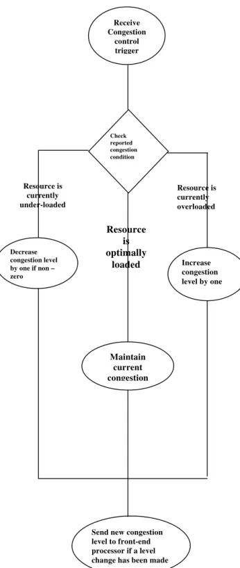
CSMA/CA (carrier sense multiple access/collision avoidance) In CA (collision avoidance), collisions are avoided because each node signals its intent to transmit before actually doing so [3]. This method is not popular because it requires excessive overhead that reduces performance. Figure 1 below, describes the basic algorithm for congestion control.
A. The congestion control task will receive a congestion trigger if the any of the resources being monitored crosses a congestion threshold, i.e. congestion has either risen above a threshold or fallen below a threshold [1].
B. On the basis of the reported congestion condition, the congestion control task applies a congestion level.
o Resource Overloaded: If the monitored
resource is overloaded, the traffic in the system needs to be reduced. Thus, the congestion control task increases the throttling of traffic by increasing the congestion level by one.
o Resource Optimally Loaded: If the
Fig 1 Basic Algorithm for Congestion Control.
o Resource Under Loaded: If the monitored resource is
under loaded, the system can handle more traffic than is being currently offered. Thus, the congestion control task decreases the throttling of traffic by decreasing the congestion level by one.
C. If the congestion level has changed in the previous step, the task needs to implement the level change by asking the front-end processors to increase or decrease traffic blocking.
D. The front-end processors take appropriate action. This action will result in change in traffic load.
Changes in load handled by the system will finally result in further congestion triggers, thus bringing us back to point 1.
Concept of Routing Algorithm
Routing algorithms can be differentiated based on several key characteristics. First, the particular goals of the algorithm designer affect the operation of the resulting routing protocol. Second, various types of routing algorithms exist, and each algorithm has a different impact on network and router resources. Finally, routing algorithms use a variety of metrics that affect calculation of optimal routes. The following sections analyze these routing algorithm attributes.
II. THE DIJKSTRA’S ALGORITHM
The Dijktra’s algorithm is one of the standard algorithms that determine the shortest route between any two nodes, towns or villages in a Local Area network, road network respectively. It also determine the most efficient message route between each, two geographic area in a GSM network.
The Dijktra’s algorithm uses a special labeling convention to label the various nodes of the network. It begins by labeling the nodes temporary and proceeds until all the nodes have been labeled, permanent. The Dijktra’s algorithm determines the shortest route between a particular node in the network. The special labeling convention that Dijktra’s algorithm uses is of the form T[a,b]c, or P[a,b]c, T, means a temporary label, a, is the distance between the source node and the node you are labeling, c, while b, is the node sequence or the node that will be followed in order to reach the node you are labeling.
The Dijkstra’s algorithm terminates when you have labeled all the nodes as permanent labels, but it begins by labeling the source node with the permanent label, P[0,-]s, 0, in this label means that the distance from the source node to the node s, P, denotes a permanent label, while, -, means that there is no sequence node to the source node. Mathematically, we can formalize the Dijkstra’s algorithm as follows:
1. Initialization:
The first steps of Dijktra’s algorithm inializes all variables and sets that will be used. The following variables and sets will be initialized as follows: The Variable, I, will be initialized as the source node.
The set, Cj, will be initialized to empty, this set will be used to determine the nodes that have not been labeled permanently and can be reached directly from the source node, this means that Cj is the of all nodes that have not been labeled permanently, and can be reached directly from the node, i.
The set, Ct will be initialized to empty, this set will be the set of all temporary labeled nodes. The set Cp, will be initialized to empty, this set will be the set of all permanently labeled nodes.
Resource is currently overloaded Receive
Congestion control trigger
Decrease congestion level by one if non – zero
Increase congestion level by one
Maintain current congestion
Send new congestion level to front-end processor if a level change has been made
Check reported congestion condition
Resource is currently under-loaded
Resource is optimally
2. Labeling the Source Node:
Label the source node as follows: P[0,-]I and insert this label into the set of permanently labeled set. Therefore, the set of permanently labeled node becomes Cp = {[0,-]}.
3. Determination of Set, Cj:
Determine the set, Cj, this is the set of nodes that have not been labeled permanently, and can be reached directly from node, I, mathematically, we express this set as follows: Cj = {j э∑ (I,j)^j ¢ Cp}
4. Labeling of the Nodes in Cj temporary:
Suppose the set, Cj is not empty, then the nodes in the set, Cj will be labeled temporary. To do this, follow these steps.
Count the elements in set, Cj. Use the variable, cnt to hold the number of elements in set, Cj.
Initialize a count variable to zero i.e cto = 0.
Label a node j in set Cj, temporary as follows: T[a+dij,i], where a , is the distance label in the permanent label of node I and dij is the distance between node I and node j. If this node has been labeled temporary, previously, pick the label with the minimum distance.
Make this temporary label of node j a member of the set of temporary labeled set. This can be expressed as follows: insert (T[a+dij,i}j,Ct), provided that it is not in set, Ct, otherwise, you do not need insert it into Ct.
Increase the Count Variable: Add 1 to this Variable, cto, this means that cto = cto +1.
5. Repeat 4.3, 4.4, 4.5 until cto equal ctn
6. Labeling a Node in Temporary Set, Ct, Permanently: Among all the temporary labeled nodes in the set, Ct, pick the node label that has the minimum distance, and label it permanently, after this, remove the node from set of temporary labels, and insert it into the set of permanent labels. This can be expressed in the following smaller steps, under steps 5.
Pick node with minimum distance. Pick node j, with minimum distance from set, Ct. This can be expressed as follows: element (Min {T[a,b]c}, Ct).
Remove it from temporarily labeled set Ct, this can be expressed as follows: remove(T[a,b]j, Ct).
Label it permanently: Label the node, j that you have picked, permanently. This can be expressed as follows: P[a,b]j.
Insert the new permanently labeled node into the set of permanent labels, this can be expressed as follows: insert (P[a,b]c, Cp).
7. Let I = j and repeat steps 3, 4 and 5, until the temporary labeled set, Ct becomes empty.
III. IMPLEMENTATION OF DIJKSTRA’S ALGORITHM Global system for mobile communication (GSM) uses a Satellite network technology with computerized switches in each cell that covers a certain geographic area, with a transmission tower that links a central telephone switching office. These transmissions towers from the GSM network. Chang, C.S (2000).
The GSM Satellite network technology routes messages through the central telephone switching office and the various transmission towers that forms the GSM network, in an efficient manner[4],[5]. Moreover, routing of messages in a GSM network uses the same HDLC, High Data Link Control,
a data link protocol that the lands’ Public Switch Telephone Network uses. HDLC has the shortest route algorithm as one of its algorithms that establishes the most efficient message route. [3] In order to consider the problem of congestion , this scenario is considered. The Glo-Mobile Phone Company services six geographical areas in Nigeria. The satellite distances (in miles) among the six areas are given in the network diagram in fig 2. Glo-Mobile needs to determine the most efficient message routes that should be established between each two areas in the network.
2
4 9
3
5
10
7
6
8
Fig 2 Glo-Mobile Network Diagram Using Dijkstra’s Algorithm To solve these problems using the Dijkstra’s algorithm, it is necessary to consider a particular node in the network, and then find the shortest route between that node and any other node in the network. The reason for this is because the Dijkstras’ algorithm gives us the shortest route between a particular node and any other node in the network [8]. IV. RESULT GENERATED USING THE SOFTWARE DESIGNED The following are result obtained when the software developed were subjected to problem, using Dijkstra’s algorithm, consider node 1 as the source node we precede as the algorithm specifies T[4,1]2 T[6,2]4 T[14,3]]2 T[15,3]4 T[17,4]2 P[6,2]4 P[4,1]2 2
4
9 10 3
6
p[0 --,]1 8
T[5,1]3 T[13,3]5
T[13,3]]3 T[9,4]5 T[16,4]3 P[9,4]5 P[5,1]3
Fig 3 Labeled Nodes
T[13,4]6
T[19,4]6
P[13,4]6
T[6,2]4
T[14,3]]2
1
6
2
4
3
5
1
6
2
4
Having labeled the entire nodes and the set of temporary labeled nodes becoming empty, the Dijkstra’s algorithm stops which the following as the set of permanently labeled nodes. Cp = {[0,-]1,[4,1]2,[5,1]3,[6,2]4,[9,4]5,[13,4]6}
Using this set of permanently labeled nodes, the shortest route between node 1 and any other node can easily be determined with its appropriate distance. Shortest route between node 1 and node 6 can be shown below:
Total distance is 13 miles
Fig 4 Routes between nodes
To determine this shortest path from the set of permanently labeled nodes, it is necessary to use the sequence node that the label specifies. Similarly, the set of permanently labeled nodes can be used to determine the shortest route between node 1 and node 5, as follows in Fig 5
Fig 5 Labeled nodes
V. RESULT GENERATED USING THE SOFTWARE DESIGNED
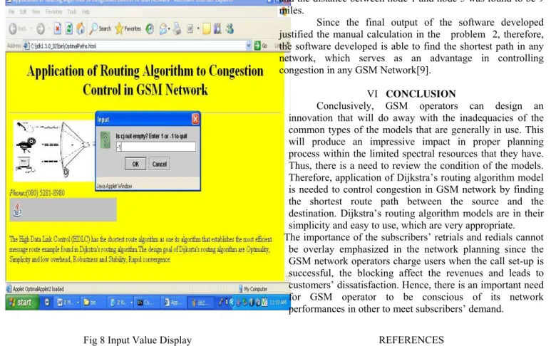
The following are the final results obtained as both input and output values displayed when using the software for the problem:
Fig 6 Determination of the set
Fig 7 Output Value Display Window
1
2
4
6
4
2
7
1
2
4
5
Fig 8 Input Value Display
A. Analysis of Results
Fig 3 explained the operation to continue the processes by pressing 1 or –1 to quit provided that the set of nodes that have not been labeled permanently and can be reached directly from node,i. , are not empty.
In Fig 5, the numbers of the set of Cj were determined shows the input dialogue box to input the node numbers and their distances. After the input of the whole node number and their distances, the minimum distance and its distance were obtained .
The new node is now considered as the permanent node and at the same time the new source node. The same operation, which was carried out on formal source node 1, was still repeated on the new source node to determine another permanent node as shown in Fig 5-7. The final result, which is the shortest distance in miles, is now gotten to solve both the problem 1 and problem 2 as shown in Fig 8.
The performance of Dijkstra’s routing algorithm is extensively examined and critically investigated in this chapter. The results obtained from the problems is hereby analyzed and commended on. The Dijkstra’s algorithm when used on each of the problems shows that the Dijkstra’s algorithm will always need a source node to find the distance between any two nodes i.e. to find the distance between two nodes, you need a source node which means that only the distance between that source node and other nodes can be found.
.For problem 2, using 1 as the source node the distance between node 1 and node 6 was found to be 13 miles
and the distance between node 1 and node 5 was found to be 9 miles.
Since the final output of the software developed justified the manual calculation in the problem 2, therefore, the software developed is able to find the shortest path in any network, which serves as an advantage in controlling congestion in any GSM Network[9].
VI CONCLUSION
Conclusively, GSM operators can design an innovation that will do away with the inadequacies of the common types of the models that are generally in use. This will produce an impressive impact in proper planning process within the limited spectral resources that they have. Thus, there is a need to review the condition of the models. Therefore, application of Dijkstra’s routing algorithm model is needed to control congestion in GSM network by finding the shortest route path between the source and the destination. Dijkstra’s routing algorithm models are in their simplicity and easy to use, which are very appropriate. The importance of the subscribers’ retrials and redials cannot
be overlay emphasized in the network planning since the GSM network operators charge users when the call set-up is successful, the blocking affect the revenues and leads to customers’ dissatisfaction. Hence, there is an important need for GSM operator to be conscious of its network performances in other to meet subscribers’ demand.
REFERENCES
[1] D., Anick, D. Mitra, and M. Sondhi, (1982) Stochastic Theory of Data. Handling system with multiple sources, Bell System Technical Journal, Vol. 61, No. 8, pp. 1871-1894
[2] Chang, C.S (2000) “Performance Guarantees in Communications Network”, Springevverlay,NY pp. 112-150
[3] Geijer-Lundin (2003) “Uplink load estimates in WCDMA with different availability of measurements.” Pro. IEEE Vehicular Technology Conference Spring.
[4] GSM-Technik and Messpraxis [GSM technology and practical testing in German] ± Red1/Weber,Franzis’,Poing
[5] Gunnarsson and Gustafsson (2002) “Power Control in cellular radio system from a control theory perspective.” Survey paper. IFAC World Congress. [6] Gunnarsson (2003) “Adaptive filtering applied to an uplink load estimate
in WCDMA.” Pro. IEEE Vehicular Technology Conference Spring. [7] Gustafsson (2003) “Controlling internet Queue Dynamics using
Recursively Identified Model.” Pro. IEEE Vehicular Technology Conference Spring.
[8] Microcells in mobile communications Tibor RakoÂ,Gyo Zo Drozdy http://www.pgsm.hu/english/gsm/more.html.
[9] Mobilkommunikation,Hochschulkolleg[Mobile Communications, High-school textbook in German] Ulrich Bochtler, Walter Buck, Eberhard Herter; Steinbeis Transferzentrum, Kommunikationszentrum Esslingen. [10] John Scourias Overview of the Global System for Mobile
Communications, University of Waterloo; http://ccnga.uwaterloo.ca/~jscouria/GSM/gsmreport.html